Visualizing shifts in Founder Assignment for an Admixed Population of Mice caused by a New Genomic Build
By Peter Jinchan Fan
Senior Honors Thesis Biology
University of North Carolina at Chapel Hill
4/22/2016
Approved:
_____________________________
Leonard McMillan, Thesis Advisor
Greg Copenhaver, Reader
Abstract:
Populations of inbred laboratory mice are highly desirable as model organisms due to their
easily reproducible (isogenic) genomes. A combination of SNP genotyping arrays and a hidden Markov
model (HMM) algorithm have been used successfully to accurately determine the genetic architecture
of inbred mice. This HMM algorithm, known as the Founder Assignment algorithm, performs
statistical modeling on genotyping data to calculate the probability that a given segment of a mouse’s
genome was inherited from a particular founding strain of the population. However, the predictions
generated by this algorithm are sensitive to changes in the genomic positions of the SNP markers used
for genotyping. Although many groups have worked to improve the accuracy and resolution of HMM
algorithms, few have considered how new assemblies of the genome, in which entire sets of markers
may be reordered or removed, affect HMM predictions. In this study, the Founder Assignment
algorithm was adapted to work with a new assembly (Build 38) of the mouse genome. The algorithm
was then run on a collection of genotyping data from approximately 400 mice. A new visualization
tool, which more clearly displays the HMM probabilities, was developed in order to identify regions
where the algorithm assigned different founders between Build 38 and the previous build. In the future,
these insights will help us design versions of the algorithm to work with newer versions of the
Introduction
The Collaborative Cross (CC) is a collection of admixed mouse populations that were
established by crossing and inbreeding eight genetically diverse “founder” strains of mice3,5,6.
Altogether, these founder strains capture nearly 90% of known genetic variation present in the genomes
of laboratory mice6. In addition, due to generations of inbreeding, these CC mice have genomes which are readily reproducible (isogenic)5. As a result, CC mice are often used as model organisms in a variety of genetic tests including studies on drug-gene interactions and the interplay between genes and
the environment3. In order to fully understand these complex genetic interactions, it’s important to first have an accurate representation of a given CC mouse’s genome. Before the advent of high-throughput
sequencing, the primary method to obtain this knowledge was the use of a genotyping array.
Genotyping arrays are essentially multi-welled plates with a single DNA “probe” affixed to the
bottom of each well11-13. Each of these DNA probes is complementary to a specific SNP (single
nucleotide polymorphism), a genetic variant or allele that is present in a subpopulation of the mice. To
test for the presence of these genetic variants, DNA from the mouse of interest is bound with a
fluorescent tag and mixed onto the array. Sequences which are complementary to the DNA probes will
hybridize (bind) to the probes and become immobilized. Non-hybridized DNA is removed via a
washing step and the presence/absence of particular SNPs is determined using a technique, such as
fluorescence microscopy, to measure the fluorescence of each well. A genotyping array known as the
Mouse Universal Genotyping Array (MUGA) was developed alongside the Collaborative Cross in
order to obtain an accurate picture of the genetic variation present in individual inbred mice11-13. The original MUGA array was designed to identify only ~7,800 SNPs. It’s successor, MegaMUGA, was
used in this experiment to genotype several hundred mice at ~78,000 different “marker” SNPs
Purpose and Advantages of the Collaborative Cross
The Collaborative Cross was developed as a Genetic Reference Population (GRP) for the Mus
musculus laboratory mouse4. Although there are other mouse GRP’s, the Collaborative Cross was specifically developed with the field of systems genetics in mind and has several advantages over these
other GRP’s4. Most notably, each strain in the Collaborative Cross has a nearly even distribution of genomic regions from each of the 8 founder strains whereas most GRP’s only consist of the inbred
progeny of two founding strains. In addition, 5 of the founding CC strains were classically inbred
laboratory strains while 3 were wild-type subspecies of M. musculus mice. Consequently, each inbred
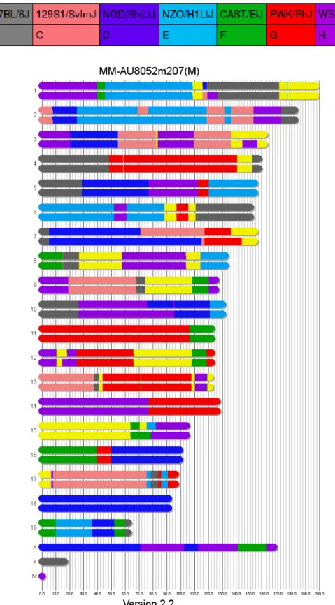
line shows a high amount of both genetic variation, which is spread evenly throughout the genome (see
Figure 1), and phenotypic variation4.
As a result, CC mice are a good model of the genetic diversity present in humans and are
extremely useful for Quantitative Trait Loci (QTL) mapping and Genome-Wide Association Studies
(GWAS)7,8,10. These two techniques are often employed to study diseases that have complex etiologies involving elaborate gene networks or gene-environment interactions4,7. Examples include various cancers, heart disease, and diabetes. These techniques aid in deciphering these disease etiologies by
identifying candidate genes or genomic regions which are associated with the conditions and which
could play a causal role in their etiologies4,7. However, in order to use these mice for QTL mapping and GWAS, the genomes for each inbred line must first be mapped. The preferred method for obtaining this
mapping is a combination of SNP genotyping and ancestry inference using hidden Markov model
Figure 1.A visual representation of the Founder Assignment algorithm output for an example CC mouse. The x-axis represents the length of the DNA in
Because each CC mouse is a descendant of one or more of the eight founder strains, each
segment of a given mouse's genome can be traced back to one of these eight founders11,12. Since each of the eight founding strains has been sequenced, identifying the ancestral origin of each genomic region
provides a picture of the specific ordered collection of genes (aka haplotype) present in that region1,2. This ancestral origin can be determined using data on the SNPs present in a given mouse’s genome.
Each of the eight founding strains has different SNPs at different loci in the genome. As a result, the
ancestral origin of each segment of a given mouse’s genome can be identified by genotyping the SNPs
at the loci flanking the region and identifying which of the eight founders those particular SNPs are
most likely to have come from11,12. The probes used in the MUGA and MegaMUGA genotyping arrays were specifically chosen to identify certain SNP “markers” in the genome that would allow users to
discriminate between the different founders at regular intervals throughout the genome4.
Hidden Markov model algorithms
In order to predict the ancestral origin of each genomic region, this SNP genotyping data was
fed into a hidden Markov model (HMM) based algorithm known as the “Founder Assignment”
algorithm4,11,13. An HMM is a statistical model used to study phenomena which can take on a number of different unknown or “hidden” states. In this case, the founders which contributed a particular region of
the genome was the hidden state. Because there are 8 CC founders, there are 8 possible homozygous
combinations and 28 possible heterozygous combinations that could have produced a given genomic
region for a total of 36 possible hidden states. To assign founders to the different genomic regions, the
algorithm iterates through the genotyping data and, at each locus that was genotyped, calculates the
probability that each of the 36 possible hidden states could have produced the genotype found at that
locus.
and a transition probability4,11. The emission probability is calculated by looking at the genotyping data and calculating the probability that each of the 36 possible hidden states could have produced the
genotype present at that particular locus. On the other hand, the transition probability is the probability
that the model could be in a given hidden state at a particular locus given the hidden state at the
previous locus. This transition probability is typically highest for the “no transition” situation--the
situation where the hidden state at a particular locus is exactly the same as the hidden state at the
previous locus11,12. The transition probability accounts for the fact that it’s generally more likely that a given founder contributed a single longer region of the genome rather than several founders each
contributing short regions.
Though many research groups have worked on improving the resolution or efficiency of this
algorithm, none have considered the potential impact that a different assembly of the mouse reference
genome could have on the predictions generated by the algorithm. Since the emission and transition
probabilities utilized by the HMM are sensitive to the order and location of the marker SNPs, a
different assembly of the genome, in which whole blocks of SNPs may be deleted or moved around,
could produce serious errors in the predictions generated by the algorithm. As a result, the goals of this
study were:
1. To adapt an HMM algorithm for MegaMUGA and Build 37 of the mouse reference genome to
work with a new assembly of the mouse genome (Build 38).
2. To develop a new visualization tool to identify regions where the largest changes in HMM
prediction probabilities between builds occur.
A better understanding of the differences in predictions between builds would provide insight
into ways to refine the algorithm or redesign the genotyping arrays to account for these changes and
Methods
In order to determine the effects of a new assembly of the mouse genome on the Founder
Assignment algorithm’s predictions, the Founder Assignment algorithm was first adapted to work with
a new assembly. This process was primarily computational and can be broken down into the following
steps:
I. Identified MegaMUGA SNP markers in Build 38
In every new assembly of a genome, the position of certain genetic elements shifts as parts of
the genome are shortened, lengthened, moved around, or deleted entirely. As a result, the positions of
each of the SNPs used as markers for MegaMUGA had to be located in the Build 38 version of the
mouse genome. This work was completed primarily by a graduate student in the lab who assembled the
results into a CSV (comma separated value) file.
II. Filtered out markers that were no longer unique
Every SNP in MegaMUGA was selected as a marker both for its ability to differentiate between
founders and its uniqueness in the genome. In other words, in order for the genotyping array to
accurately identify the SNPs present in a given mouse, the probe for a given SNP marker should only
bind to a single location in the mouse genome. In Build 38, it was discovered that a number of the
markers that were identified as unique in Build 37 were no longer unique. These non-unique markers
were filtered out using a short Python script. This script iterated through the original CSV, selected
Build 37 markers which only had a single genomic position in Build 38, and generated a new CSV
III. Modified Founder Assignment algorithm to accept Build 38 positions as input
The Founder Assignment algorithm had several hard-coded dependencies which made it only
able to accept Build 37 marker positions as input. As a result, it had to be modified to work with Build
38. The key difficulty in this reconfiguration was caused by the markers that were no longer unique and
had been filtered out in the previous step. Because these filtered markers were spread throughout the
genome, a large number of SNPs were matched with the wrong genomic position by the algorithm
causing the HMM to produce nonsense probability data. As a result, a “look-up table” data structure
was added so that unique markers in Build 37 could be matched with their Build 38 positions and
removed markers could be filtered out.
IV. Ran the Founder Assignment algorithm on 409 CC mouse samples
The Build 38 configured Founder Assignment algorithm was run on 409 different CC mouse
samples that had already been run with Build 37. A single mouse sample consisted of all the genotypes
for the ~78,000 different MegaMUGA SNPs for the given mouse. Mouse sample data was retrieved
from an SQLite database. The Founder Assignment algorithm returned its results in the form of a CSV
file detailing the probability that each founder could have contributed a particular SNP for every one of
the ~78,000 SNPs in a given sample.
V. Development of a new HMM probability visualization tool
After modifying the Founder Assignment algorithm to work with Build 38, a new
visualization tool was developed to identify differences between the HMM probabilities
produced by the different builds. This tool was developed using the NumPy, Pandas, and Bokeh
Python libraries and displays probabilities as a stacked area plot. The visualization tool takes a
database. Probabilities were then sorted based on their associated marker SNP’s chromosome
and location in the genome.
However, the visualizations were often slow to load due to the size of the data set. To shorten
this load time, a pruning function was developed in order to remove markers that were non-essential for
the visualization. This pruning function iterated through the data set and, for every data point,
determined whether it was possible to draw a line between the point directly before and directly after
the given data point that would pass through the data point. If so, that point was not essential for the
visualization since it would fall directly on the line between the point preceding and proceeding it.
These non-essential points were removed from the graph in order to prune the data. Although
seemingly simple, the pruning approach was effective and was often able to reduce the size of the data
by up to 80%.
Results - Analysis of numbers of unique markers between builds
After identifying the Build 38 positions for each of the MegaMUGA marker SNPs, the changes
in number of unique markers were calculated and are displayed in the table below.
A total of 98.67% of all markers were still unique in Build 38. The 1035 markers that no longer
had unique matches in Build 38 can be subdivided into markers with more than one match (95.07% of
the markers that were no longer unique) and markers with no match (4.93%). None of the unique
markers appeared to have changed chromosome, but two markers with no match in Build 37 had
matches on Chromosome 5 of Build 38.
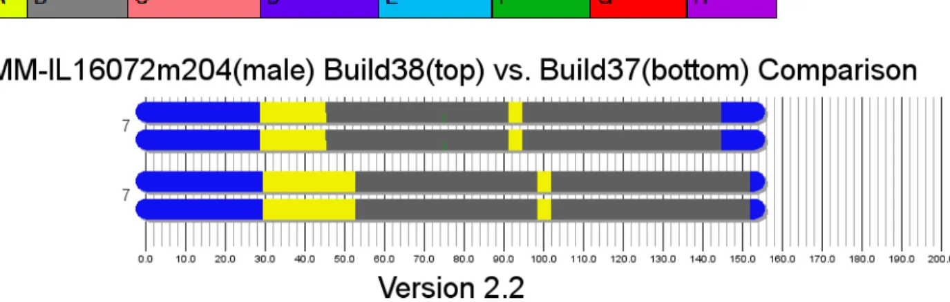
Not surprisingly, many of the differences in HMM probabilities appeared in regions where the
HMM algorithm already had difficulty assigning founders. For example, the ends of chromosomes are
notoriously difficult to genotype and a large number of samples were assigned different founders at the
ends of chromosomes. Another area of contention was the “transition regions” or loci where the HMM
algorithm predicts there will be a change from one genotype to another in Build 37. In many cases the
Build 38 algorithm extended or shortened these regions (see Figure 2 below). Further analysis is
required to determine the exact cause of these changes but a likely cause is the removal of one or more
marker SNPs in the transition region during the filtering for non-unique markers step.
Comparison of Build 37 and Build 38 using a new visualization tool
An examination of the same sample and chromosome using the new visualization tool provides
a more nuanced view of the differences between Build 37 and Build 38. In this new visualization,
probabilities are visualized as a stacked area plot. As a result, at every locus, every hidden state’s
probability calculated by the HMM is visible rather than just the hidden state with the highest
probability. In addition, the Bokeh Python library used to create the plots generates dynamic graphs
rather than static images. Consequently, it is possible to magnify regions of interest for a more detailed
look at the changes in probability.
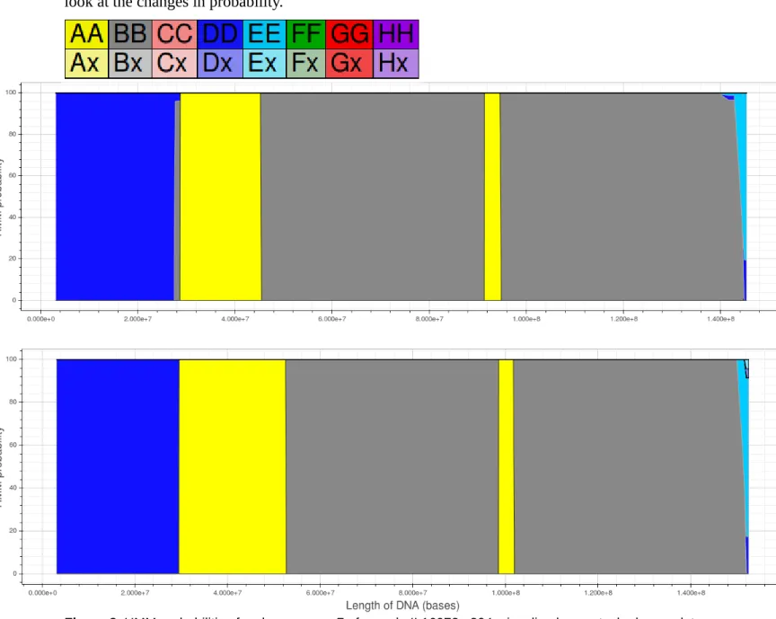
The color coding scheme for this visualization (above) is the same as the previous visualization
for all homozygous hidden states but heterozygous hidden states are color coded slightly differently.
The stacked area for every heterozygous hidden state is divided in half and each half is color coded
with a pastel version of the color associated with one of the two founders that contributed to the
heterozygous state. For example, if a given region had the hidden state AG then half the region would
be colored pastel-yellow for the A founder while the other half would be colored pastel-red for the G
founder.
The two stacked area plots above display the HMM probabilities for chromosome 7 of mouse
sample IL16072m204 generated using Build 38 (top) and Build 37 (bottom) of the genome. Although
the differences in probabilities between builds appear to be largely the same as the previous
visualization, several new details emerge in this new visualization scheme.
For example, in the Build 38 visualization of chromosome 7, a small region with a high
probability of BB, located around 28 Mb, appears which was not present in the Build 37 visualization
(Figure 4). Similarly, in the Build 37 plot, there is a region where EH is predicted with a probability of
around 10% near the end of the chromosome which disappears entirely in the Build 38 plot (Figure 5).
Discussion - Shifts in marker position
The results provide insight into the changes in HMM probabilities that can occur when running
the Founder Assignment algorithm with different assemblies of the mouse genome. Shifts in the
position of certain SNP markers are particularly interesting because hidden Markov models are very
sensitive to the position of the markers they use as input. Out of 77,808 markers that were unique in
Build 37, a total of 76,773 were still unique in Build 38. Out of the markers that were no longer unique
in Build 38, a large majority of them (984) were found to have more than one binding site in the Build
38 reference genome. A much smaller proportion (51) were found to appear nowhere in the genome in
Build 38 despite appearing in Build 37. Although a number of markers disappeared or were no longer
unique, none of the 76,773 remaining markers appear to have changed position relative to one another
or shifted from one chromosome to another.
The most interesting result of this preliminary analysis was a pair of markers that suddenly
appeared in the genome on chromosome 5 in Build 38. A subset of the MegaMUGA probes do not bind
to marker SNPs but instead target a variety of engineered genetic constructs, such as promoters and
fluorescent proteins. As a result, these markers do not have a genomic position in Build 37 because the
constructs they bind do not appear naturally in the genome. However, in Build 38, a binding site for
two of these constructs was discovered on chromosome 5 of the mouse reference genome. This
discovery suggests that the probes for these two markers could be targeting the wrong sequence or that
there was an error in the genome assembly.
Strengths and weaknesses of the new visualization tool
The new visualization tool graphs the HMM probabilities as a stacked area plot. In this
representation, the probabilities for every hidden state at a certain locus are visualized rather than just
because changes in build may affect the HMM probabilities in subtle ways beyond which founder is
ultimately given the highest probability. For example, regions where the algorithm struggled to assign a
single founder with high probability are visible in this new visualization scheme. In the previous
visualization, these regions would not have been apparent since only the founder with the highest
probability was displayed. In addition, the Bokeh Python library generates dynamic and interactive
plots rather than static images. As a result, users can magnify areas of interest or scroll over regions of
interest to retrieve additional data associated with different data points.
Although the new visualization style has many advantages, there are also several drawbacks.
These dynamic visualizations are each generated on the fly and as a result take longer to load and
process. In addition, unlike the previous static images, they cannot be cached to reduce load times for
future uses. Furthermore, since the HMM probabilities for a given chromosome are being represented
by a single stacked area plot rather than a pair of chromosomes some information on the predicted
ordering of haplotypes across the two chromosomes is lost. Finally, some of the pastel colors used for
heterozygous hidden states may be difficult to discern from one another at first glance.
Future Work
Further analysis across all samples is required to determine the exact causes of the differences
between builds. A likely cause is that the loss of markers in certain regions causes changes in the
lengths of these regions. Therefore, a good follow-up experiment would be to determine the positions
of the markers that were filtered out between builds and to see if these locations are correlated with the
regions with the largest changes between builds. A subset of the samples which experienced the largest
changes between their Build 37 and Build 38 probabilities could be identified and then visualized with
the new tool. In order to find these samples, the HMM probabilities for Build 37 and Build 38 could be
could then be plotted with the new visualization tool to determine whether regions that experienced
large changes in probability were correlated with regions where markers were lost.
Conclusion
In this study, the Founder Assignment algorithm was adapted to work with a new assembly
(Build 38) of the mouse reference genome. Changes in the number of unique markers between builds
were calculated and analyzed. The reconfigured algorithm was run on 409 CC mice which already had
HMM probability data generated using Build 37. Although a vast majority of markers remained the
same between builds, the small proportion that were filtered out caused noticeable changes in the
HMM probabilities generated by the Build 38 configured algorithm. In order to better examine the
changes caused by switching builds, a new visualization tool was developed to display the probabilities
for every hidden state at every locus rather than just the founder with the highest probability. These
new dynamic visualizations were shown to be effective in identifying new details that were not visible
in previous visualizations. Further analysis of the data must be conducted in order to identify the exact
causes of the differences in HMM probabilities produced by switching genomic builds.
Acknowledgements
I’d like to thank my thesis advisor, Dr. Leonard McMillan, and the members of McMillan lab:
(Seth Greenstein, Chia-Yu Kao, and James Holt) for their patience, programming help, and mentorship.
This project built on the work of several current and former lab members. The hidden Markov model
was built by Chen-Ping Fu as part of her thesis work. In addition, the Build 38 positions for each of the
MegaMUGA SNP probes were identified by a program written by James Holt. Finally, I’d like to thank
Dr. Corbin Jones for acting as my Biology faculty sponsor, my peer editing group (Chelsea Gustafson,
References
1. Aylor, D. L., Valdar, W., Foulds-Mathes, W., Buus, R. J., Verdugo, R. A., Baric, R. S., …
Churchill, G. A. (2011). Genetic analysis of complex traits in the emerging Collaborative
Cross. Genome Research, 21(8), 1213–1222. doi:10.1101/gr.111310.110
2. Broman, K. W. (2012). Haplotype probabilities in advanced intercross populations. G3
(Bethesda, Md.), 2(2), 199–202. doi:10.1534/g3.111.001818
3. Churchill, G. a, Airey, D. C., Allayee, H., Angel, J. M., Attie, A. D., Beatty, J., … Zou, F.
(2004). The Collaborative Cross, a community resource for the genetic analysis of complex
traits. Nature Genetics.
4. Iraqi, F. A., Mahajne, M., Salaymah, Y., Sandovski, H., Tayem, H., Vered, K., … Schwartz, D.
(2012). The genome architecture of the collaborative cross mouse genetic reference
population. Genetics, 190(2), 389–401. doi:10.1534/genetics.111.132639
5. Threadgill, D. W., Miller, D. R., Churchill, G. a, & de Villena, F. P.-M. (2011). The
collaborative cross: a recombinant inbred mouse population for the systems genetic era. ILAR Journal / National Research Council, Institute of Laboratory Animal Resources,
52(1), 24–31. doi:10.1093/ilar.52.1.24
6. Threadgill, D. W., & Churchill, G. A. (2012). Ten years of the collaborative cross. Genetics,
190(2), 291–294. doi:10.1534/genetics.111.138032
7. Threadgill, D. W., Hunter, K. W., & Williams, R. W. (2002). Genetic dissection of complex and
quantitative traits: From fantasy to reality via a community effort. Mammalian Genome,
13(4), 175–178. doi:10.1007/s00335-001-4001-y
8. Wang, J. R., de Villena, F. P., Lawson, H. A., Cheverud, J. M., Churchill, G. A., & McMillan, L.
(2012). Imputation of single-nucleotide polymorphisms in inbred mice using local
9. Welsh, C. E., Hill, C., Villena, F. P. De, & Mcmillan, L. (2013). Fine-Scale Recombination
Mapping of High-Throughput Sequence Data Categories and Subject Descriptors.
Acm-Bcb, 585–594. doi:10.1145/2506583.2506642
10. Zou, F., Gelfond, J. A. L., Airey, D. C., Lu, L., Manly, K. F., Williams, R. W., & Threadgill, D.
W. (2005). Quantitative trait locus analysis using recombinant inbred intercrosses:
Theoretical and empirical considerations. Genetics, 170(3), 1299–1311. doi:10.1534/genetics.104.035709
11. Hill, C., Hill, C., Welsh, C. E., Villena, F. P. De, Hill, C., & Mcmillan, L. (2012). Inferring
Ancestry in Admixed Populations using Microarray Probe Intensities Categories and Subject Descriptors, 105–112.
12. Kao, C., Hill, C., Fu, C., Hill, C., & Mcmillan, L. (2014). InstantGenotype : A Non-parametric
Model for Genotype Inference Using Microarray Probe Intensities, 147–154.
13. Fu, C., Hill, C., Pardo-manuel, F., Hill, C., & Mcmillan, L. (2014). Quantitative Trait Loci