Thesis

(1)

Incorporating forest biodiversity and ecophysiology in watershed ecohydrologic models

By Andrea Stewart

Senior Honors Thesis

Curriculum for the Environment and Ecology University of North Carolina at Chapel Hill

April 27, 2016

Approved:

(2)

1

Abstract

Forests with species compositions that comprise different physiologic characteristics, such as stomatal conductance and xylem anatomy type, use different amounts of water and respond differently to climate conditions. In general, isohydric plants with diffuse-porous xylem anatomy are more susceptible to drought, while anisohydric plants with ring-porous xylem are less susceptible to drought and use less water. The biodiversity and spatial distribution of forests of different physiological types in the landscape may impact watershed hydrology and carbon cycling. However, few studies have used species-level ecophysiological information to inform catchment models or predict future watershed behavior. In this study, we use a spatially-distributed, process-based model, the Regional Hydro-Ecological Simulation System (RHESSys) to simulate a small water supply catchment in Chapel Hill, NC. We apply high resolution field data from the USDA Forest Service Forest Inventory and Analysis database to simulate six forest types with different physiologic types, an average forest type, and three single-tree-species forests. Results indicate that the biodiversity of forests significantly impacts streamflow quantity and patterns. Conversion of forests to diffuse-porous-dominated plants may result in decreased streamflow relative to ring-porous-dominated plants. Conversion to evergreen plants may cause fundamentally different streamflow patterns, especially in the winter months. This work will aid the modeling efforts of future local and regional water supply and help us understand the hydrologic impacts of changing forest landscapes at the species level due to changing climate and forest management actions.

Introduction

(3)

2

flood control, it has potentially negative consequences for water supply quantity given the higher consumptive rates of forested land (Farley et al., 2005). As a result, forest management can significantly impact water supplies, especially with respect to changes in forest attributes such as species composition and canopy cover.

Public water supplies in the Piedmont of North Carolina are largely dependent on surface water flows that may be abstracted directly from streams to treatment plants, or stored in reservoirs and other impoundments. Watershed models are used to estimate freshwater runoff production under different climate and land cover conditions to determine the adequacy of water supplies to current and future demand. To better understand the impacts of future land use/land change variations and forest ecosystem dynamics on water supply, we couple ecohydrological and land use/land change models to simulate streamflow patterns. These models are typically calibrated using historical climate, streamflow, and land cover data. Current models rely on the National Land Cover Database (NLCD) to classify forestland into two categories—deciduous or evergreen. However, this binary classification fails to capture forest biodiversity or the differential response of forests of different types to climate. Current canopy cover and leaf area can be specified by look-up table from land use, or can be remotely sensed. However, future or altered conditions must develop leaf area either by direct simulation, or by assimilating information from other sources. In addition, remote sensing methods cannot distinguish between species of similar life form (e.g. different species of broad leaf deciduous). Furthermore, many models assume that plant canopy foliage is constant across each forest type, failing to account for stands of varying densities, ages, and compositions. While some models do use remotely sensed plant canopy foliage data, we are unable address the case of hypothetical future or altered land cover and canopy conditions using this method.

(4)

3

spp. and Fraxinus spp. (Ford et al., 2010). In contrast, diffuse-porous wood has conduits that retain function year-round, so it has more functional sapwood area and greater water use; it limits transpiration by stomatal closure as soil become drier or atmospheric vapor pressure deficit increases. Common diffuse-porous species in the North Carolina Piedmont include Acer rubrum

and Liriodendron tulipifera (Oren and Pataki, 2001). A third type of xylem, tracheid, is present in evergreen trees such as Pinus taeda and P. echinata and has an intermediate water use and response to soil moisture (Vose et al., 2016). It is important to consider the physiological type of a forest—that is, its relative composition of tree species of various plant functional types—in order to more accurately model a forest’s response to temperature, precipitation, and soil moisture.

In addition to the physiologic type of forests, we must also consider potential future forest compositions when predicting future watershed hydrology. Different climate scenarios and forest management actions may cause different forest compositions to emerge (Elliott et al., 2015). Increased precipitation, the loss of dominant species due to tree pests and pathogens (e.g. hemlock woolly adelgid and southern pine beetle), suppression of fire, and partial cutting may lead to the rise of fast-growing diffuse-porous deciduous trees, which are opportunistic and take advantage of canopy openings, especially in wet conditions (Elliott and Swank, 2008; Elliott et al., 2015). Higher temperatures and altered precipitation patterns may modify the distribution of tree species in favor of those more adapted to xerophytic conditions, such as ring-porous species (Klos et al., 2009; Clark et al., 2012). Ring-porous species are also generally favored by regular succession, prescribed fire, and thinning of mesophytic species (Vose and Elliott, 2016). Early-succession evergreen (tracheid xylem) species may become more dominant following forest clear-cutting, which is particularly common when individuals harvest personal property for financial gain (Vose and Ford, 2011).

(5)

4

results to a modeled forest with an “average” tree type that is indistinguishable from a single physiologic type. We also aim to predict the effect of future management and climate scenarios on hydrology and carbon cycling by examining three simulated forests represented by a single tree species: Acer rubrum (diffuse-porous), Quercus alba (ring-porous), and Pinus taeda

(tracheid). This study aims to answer the following questions:

1) How does the biodiversity of forests of different physiological types influence catchment hydrology and carbon cycling in the Southeastern United States?

2) How sensitive are water yield, evapotranspiration, and forest productivity to changes in species distribution and composition?

Methods Study Area

Our study site was the Cane Creek Watershed located in southwestern Orange County, North Carolina, within the Piedmont region of the state (USGS gage 02096846; 35° 59’ 14” N, 79° 12’ 22” W) (Fig. 1). Elevation in the 19.62 km2 catchment ranges from 155 m to 240 m with a mean elevation of 196 m (U.S. Geological Survey). Cane Creek is fairly flat; mean slope is 3.5 degrees and ranges from 0 to 18 degrees. Mean annual temperature is 14.6 °C and seasonally ranges 3.5 to 25.3 °C (State Climate Office of North Carolina). Mean annual rainfall is approximately 1200 mm, though a noteworthy drought occurred during the study period in 1998-2002 (Weaver, 2005). Soils are primarily silt loams in the Carolina Slate Belt (Natural Resources Conservation Service, USDA).

(6)

5

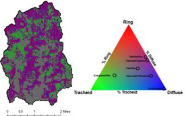
Figure 1. Cane Creek Watershed boundary, satellite imagery, and its location within Orange County and North Carolina (U.S. Geological Survey; ESRI; TomTom North America).

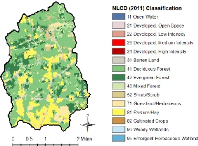
Figure 2. Land cover in Cane Creek Watershed based on the 2011 National Land Cover Database (Homer et al., 2015).

Forest Vegetation Data

(7)

6

plots during “leaf-on” season and classify plots into forest community types that are highly correlated with ecosystem properties (Schulz, 2003). FIA plots include both public and private land, but their precise location is not released to the public in accordance with the Food Security Act of 1985 and to address concerns about plot integrity and vandalism (U.S. Department of Agriculture, Forest Service, 2014). However, the data can be summarized in statistical reports and extrapolated over a broad area via a “most similar neighbor” approach using canonical correlation analysis to provide estimates of the spatial distribution of forest communities and abundance (U.S. Department of Agriculture, Forest Service, 1992). FIA data for our study was available in two forms: 1) a species summary table for each forest community, and 2) spatial realizations of forest communities.

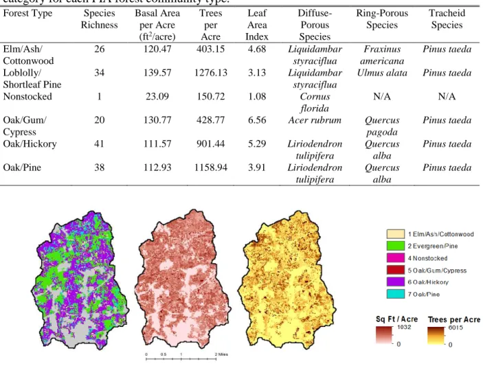
The species summary table lists the typical tree species present in each of six forest community types—Elm/Ash/Cottonwood, Loblolly/Shortleaf Pine, Nonstocked, Oak/Gum/Cypress, Oak/Hickory, and Oak/Pine (Appendix A). Mean basal area per acre and mean trees per acre are provided for each size class (greater than or equal to 11 inches and less than 11 inches) of each species. We first classified each species as having diffuse-porous, semi-diffuse-porous, ring-porous, semi-ring-porous, or tracheid xylem (Panshin and de Zeeuw, 1970; Coder, 2014). Next, we applied allometric equations to estimate the leaf area index (LAI), a measure that characterizes plant canopies and evapotranspiration potential, of each tree species (Clark et al., 1986; Chen et al., 1997; Naidu et al., 1998; Norris et al., 2001; Sabatia, 2007). We applied a correction to the logarithmic allometric equations to reduce systematic bias (Baskerville, 1971). Then, for each forest type, we calculated the total LAI for all species of each type of xylem and normalized this value by the forest type’s total LAI to develop a xylem index—the proportion of total LAI composed of each type of xylem. The full workflow for the calculation of the xylem index is available in Appendix B. Sources for allometric equations and specific leaf area values are available in Appendix C.

(8)

7

forest community type, basal area per acre value, and stand density value. To reduce computational load, we created a single map of forest communities by adopting the most common pixel ID for each pixel in the 20 realizations. Finally, we created a map of LAI across the watershed. Assuming that each pixel has the same tree species composition, size distribution, and density as the mean forest community, we calculated the proportion of total basal area per acre and total trees per acre from each tree species in each forest community. Then, to calculate the LAI for each pixel, we followed the workflow in Appendix B, this time multiplying the pixel’s basal area per acre and trees per acre by its proportion of total basal area per acre and total trees per acre in that forest type to obtain each species’ theoretical basal area per acre and trees per acre in that pixel. The full workflow for the calculation of the LAI map is available in Appendix D. Due to the logarithmic nature of allometric equations, some LAI results became unbounded; to create a reasonable LAI map, we set all pixels with LAI greater than 10 to 10, an acceptable change given that less than 2% of all pixels had LAI greater than 10.

Model: Regional Hydro-Ecological Simulation System

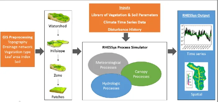
To evaluate the effect of various forest scenarios on watershed hydrology and carbon dynamics, we employed the Regional Hydro-Ecological Simulation System (RHESSys) model, a process-based and geographic information systems-based model that is structured as a spatially nested hierarchical representation of the landscape from the patch to full watershed scale (Fig. 3) (Band et al., 1993; Tague and Band, 2004). RHESSys simulates ecosystem carbon, water, and nitrogen cycling and export in complex terrain and is partially based on the MTN-CLIM, BIOME-BGC, and CENTURY models (Running et al., 1987; Running and Hunt, 1993; Parton et al. 1996). Primary model inputs include precipitation, temperature, elevation, soils, land use, vegetation type, LAI, and soils data. RHESSys also relies on a library of parameters to model the behavior of various types of vegetation, soil, and land use. Model outputs can include time series of streamflow, evaporation, transpiration, subsurface storage, baseflow, LAI, precipitation, photosynthesis, and other processes at temporal scales ranging from hourly to yearly and spatial scales ranging from patch to basin. RHESSys code is available online at https://github.com/RHESSys/RHESSys. We also used RHESSysWorkflows to aid in the development of RHESSys models (https://github.com/selimnairb/RHESSysWorkflows).

(9)

8

1. Six Unique Forests: We represented the 6 unique FIA forest types present in the study area—Elm/Ash/Cottonwood, Loblolly/Shortleaf Pine, Nonstocked,

Oak/Gum/Cypress, Oak/Hickory, and Oak/Pine.

2. Average Forest: The entire watershed was simulated as a single forest type that represented a weighted average of the 6 unique forest types.

3. Red Maple: All forest land is converted to red maple trees. 4. White Oak: All forest land is converted to white oak trees. 5. Loblolly Pine: All forest land is converted to loblolly pine trees.

Be default, RHESSys will use the NLCD and reclassify each pixel as a particular strata—non-vegetated, grass, deciduous forest, or evergreen forest. While RHESSys can accommodate multiple strata per pixel, in this study we only considered methods with a single strata per pixel to attempt to achieve desired model behavior with minimal computational rigor. The current RHESSys library has “vegetation definition files” that define the vegetation parameters for these strata. Because this method does not take into account species biodiversity across the watershed and simply represents a generalized deciduous and evergreen tree that is not specific to the particular study area, we created new vegetation definition files for each of the five models. For the Six Unique Forests model, we identified the species in each xylem type that contributed most to LAI for each of the six forest types. Then, we researched new vegetation parameters for each of these species, referencing the BIOME-BGC database and field experiments in Coweeta Hydrologic Laboratory and Duke Forest (White et al., 2000). To create a vegetation parameter file for each forest type, we weighted the parameters of the diffuse-porous, ring-porous, and tracheid species’ parameters by their xylem index. To create the Average Forest vegetation parameter file, we weighted the vegetation parameter of each of the six unique forest type parameter files based on the forest’s contribution to total LAI, plant carbon mass, leaf carbon, leaf and stem carbon, or fine root mass, depending on the nature of the vegetation parameter. To create the vegetation parameter files for the Red Maple, White Oak, and Loblolly Pine models, we referenced the parameters we researched to create the Six Unique Forests model’s vegetation parameter files.

(10)

9

age. We used the aforementioned LAI map created using FIA data as the LAI input (Appendix D) for all five models. Additionally, elevation data was provided by the National Elevation Dataset (U.S. Geological Survey), climate data was extracted from the co-op Station 311677 – Chapel Hill 2 W records (State Climate Office of North Carolina), soils data came from the Natural Resources Conservation Service’s Soil Survey Geographic Database, and additional land cover data came from the 2011 NLCD (Homer et al., 2015) (U.S. Geological Survey).

We calibrated model parameters for the Six Unique Forests model and the Average Forest model with RHESSysCalibrator (https://github.com/selimnairb/RHESSysCalibrator). Two thousand calibration iterations were completed for each model with a spin-up period of five water years (1992-1997). We calculated daily Nash-Sutcliffe Efficiencies (NSEs), daily log NSEs, weekly NSEs, weekly log NSEs, monthly NSES, yearly NSEs, total bias, summer bias, and winter bias for all calibration iterations. To choose 20 parameter sets for further analysis, we first selected all parameter sets with less than 20% total bias, summer bias, and winter bias and with all NSEs greater than 0. We selected half of the remaining parameter sets based on which iterations had the lowest total bias. We selected the other half of the remaining parameter sets based on which iterations had the highest weekly NSEs due to the importance of weekly flows for water supply. The parameter sets chosen for the Six Unique Forests model were used for the Red Maple, White Oak, and Loblolly Pine models.

(11)

10

Data Analysis

We ran each model using its top 20 parameter sets and analyzed the following daily outputs at the basin scale: streamflow, transpiration, evaporation, net photosynthesis, LAI, saturation deficit, and precipitation. We considered the values in a 95% confidence interval across the 20 model runs. To more easily compare model results and ascertain overall patterns, we analyzed aggregated outputs by calculating annual or mean monthly output values. All analysis was completed in R (R Development Core Team, 2008).

Results Vegetation

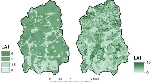
By creating a modal spatial layer of FIA forest cover, basal area, and stand density, we found that 3.1% of forest was Elm/Ash/Cottonwood, 34.5% was Loblolly/Shortleaf Pine, 0.1% was Nonstocked, 0.88% was Oak/Gum/Cypress, 48.6% was Oak/Hickory, and 12.8% was Oak/Pine (Fig. 4). Across the watershed, the basal area and stand density peaked at lower values, around 100 ft2/acre and 250 trees per acre, respectively (Fig. 5). By applying allometric relations to the basal area and tree density, we obtained a novel LAI map (Fig. 6), which provided much greater spatial diversity and a larger range of LAI values than the previous methods (Fig. 7).

We found the species richness, total basal area per acre, stand density, LAI, and the species of each xylem anatomy that contributed most to LAI for each FIA forest type (Table 1). Oak/Gum/Cypress had the greatest LAI of 6.56, largely due to the dominance of Quercus pagoda (Cherrybark Oak). Nonstocked had the lowest LAI due to the low basal area and the fact that all individuals were small (less than 11 inches diameter at breast height). While Pinus taeda

(12)

11

By calculating xylem indices for each forest type, we found that Oak/Gum/Cypress and Oak/Hickory had fairly similar distributions of species of xylem types (Fig. 9). The spatial distribution of these xylem indices is mapped by color gradient in Figure 10. Oak/Pine and Loblolly/Shortleaf Pine had an increased presence of tracheid xylem. Elm/Ash/Cottonwood and Nonstocked forests exhibited a greater diffuse-porous presence. Note that Nonstocked forests only had one species, Cornus florida, causing a xylem index of 1 for diffuse-porous. The new vegetation parameter files that were developed based on these indices and other research are available in Appendix E.

Table 1. Summary of the typical number of unique species, total basal area per acre, total stand density, leaf area index, and species that contributed most to LAI in each xylem anatomy category for each FIA forest community type.

Forest Type Species Richness

Basal Area per Acre (ft2_/acre)

Trees per Acre Leaf Area Index Diffuse-Porous Species Ring-Porous Species Tracheid Species Elm/Ash/ Cottonwood

26 120.47 403.15 4.68 Liquidambar

styraciflua Fraxinus americana Pinus taeda Loblolly/ Shortleaf Pine

34 139.57 1276.13 3.13 Liquidambar styraciflua

Ulmus alata Pinus taeda

Nonstocked 1 23.09 150.72 1.08 Cornus

florida

N/A N/A

Oak/Gum/ Cypress

20 130.77 428.77 6.56 Acer rubrum Quercus

pagoda

Pinus taeda

Oak/Hickory 41 111.57 901.44 5.29 Liriodendron

tulipifera

Quercus alba

Pinus taeda

Oak/Pine 38 112.93 1158.94 3.91 Liriodendron

tulipifera

Quercus alba

Pinus taeda

(13)

12

Figure 5. Distribution of imputed FIA-based basal area per acre and trees per acre for 30-m pixels in Cane Creek Watershed.

Figure 6. A comparison of LAI using current methods (left) and revised methods from this study (right). Typically, current models reclassify the NLCD into 4 unique LAI values—0, 1.5, 5, 6. Our methods provide greater spatial variability at the pixel-level and provide a greater range of LAI values from 0 to 10.

(14)

13

Figure 8. Distribution of topographic wetness index (TWI) for 30-m pixels in Cane Creek Watershed (Beven and Kirby, 1979; Tarboton, 2004).

Figure 9. Proportion of LAI contribution by species with diffuse-porous, ring-porous, and tracheid xylem anatomy in each FIA forest community type.

(15)

14

Model Calibration

In the 6 Unique Forests model, one calibration iteration met the criteria that total bias, summer bias, and winter bias all be less than 20% and that all NSEs were greater than 0. Due to the low number of iterations that had low bias, we selected 12 parameter sets with highest weekly NSEs and 7 parameter sets with minimized total bias. Weekly NSEs in these parameter sets ranged from -0.8591 to 0.4306, and total bias ranged from -49.11 to 4.91%.

In the Average Forest model, five calibration iterations met the criteria that total bias, summer bias, and winter bias all be less than 20% and that all NSEs were greater than 0. We selected 8 parameters sets with highest weekly NSEs and 7 parameter sets with minimized total bias. Weekly NSEs in these parameter sets ranged from -0.1314 to 0.4909, and total bias ranged from -40.70% to 19.54%.

Streamflow

We calculated mean monthly streamflow for water years 1998-2010, the period of time following a five-year spin-up period that overlapped with observed stream gage data (Fig. 11). The 6 Unique Forests and Average Forest models had less streamflow than observed in January through May, approximately similar streamflow during the summer, and greater streamflow than observed in August through December. The Average Forest model exhibited streamflow closest to the observed data in January through August, at which point the 6 Unique Forests model was the closest to the observed data.

(16)

15

Figure 11. Mean monthly streamflow (1998-2010 water years) for the 6 Unique Forests, Average Forest, Red Maple, White Oak, and Loblolly Pine models. Observed data from USGS gage 02096846 is also presented for comparison (U.S. Geological Survey).

Evapotranspiration

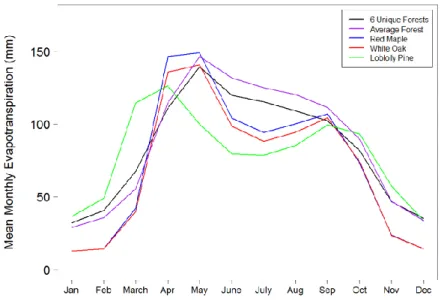
The mean monthly evapotranspiration results for water years 1998-2010 largely reflected the streamflow results (Fig. 12). Before April, the Average Forest had less evapotranspiration (ET) than the 6 Unique Forests, but the opposite trend was occurred after April. The largest differences in ET occurred in the growing season, May through September. ET for both models peaked in May.

(17)

16

Figure 12. Mean monthly evapotranspiration (1998-2010 water years) for the 6 Unique Forests, Average Forest, Red Maple, White Oak, and Loblolly Pine models.

Water Balance

The observed runoff ratio in Cane Creek Watershed is 0.20 (Table 2). The 6 Unique Forests and Average Forest models produced similar runoff ratios of 0.18 and 0.19, respectively. The Red Maple and White Oak models produced higher runoff ratios of 0.26 and 0.29 due to decreased ET. The Loblolly Pine model runoff ratio of 0.21 was close to the observed runoff ratio due to its higher ET than the other single-tree models, but its modeled streamflow was still higher than observed. The 6 Unique Forests and Average Forest may have greater change in storage than the other models due to their larger precipitation-streamflow-ET magnitudes.

Table 2. Mean annual water balance (1998-2010 water years) for the 6 Unique Forests, Average Forest, Red Maple, White Oak, and Loblolly Pine models. Observed data from USGS gage 02096846 (U.S. Geological Survey) and the Chapel Hill 2 W co-op station (State Climate Office) is also presented for comparison.

Model Observed 6 Unique

Forests

Average Forest

Red Maple White Oak Loblolly Pine Precipitation (mm) 1286.09 1286.09 1286.09 1286.09 1286.09 1286.09

Streamflow (mm) 253.08 225.38 243.47 335.96 372.77 269.12

Evapotranspiration (mm) 1033.01 1078.3 1064.41 949.79 906.16 1027.6

P-Q-ET (mm) 0.00 -17.59 -21.78 0.35 7.16 -10.63

(18)

17

Saturation Deficit

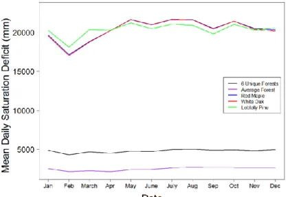
We examined the mean daily saturation deficit depth, or depth to water table, for each model (Fig. 13). The water table in the 6 Unique Forests and Average Forest remained relatively constant throughout the year, though the 6 Unique Forests water table was lower than that of the Average Forest. The water tables for the single-tree models were approximately five times deeper and more variable over the year, highest in February. The saturation deficit for the Red Maple and White Oak models was nearly identical over time. The Loblolly Pine model experienced less variability over time; its range was less than that of Red Maple and White Oak by about 25%.

Figure 13. Mean daily saturation deficit (1998-2010 water years) for the 6 Unique Forests, Average Forest, Red Maple, White Oak, and Loblolly Pine models. Note that the Red Maple and White Oak line are overlapping.

Carbon Dynamics

(19)

18

Net annual canopy photosynthesis, the net amount of primary production after accounting for the cost of plant respiration, was very similar for the 6 Unique Forests, Average Forest, and White Oak forest at around 1.45 kg C per square meter (Fig. 15). Net annual photosynthesis in the Red Maple forest was 0.92 kg C per square meter, while the Loblolly Pine forest had the lowest photosynthetic activity at 0.61 kg C per square meter.

Figure 14. LAI patterns for the 2001-2003 water years for the 6 Unique Forests, Average Forest, Red Maple, White Oak, and Loblolly Pine models. Note that the troughs of the Red Maple line are covered by the White Oak line.

Figure 15. Mean annual net photosynthesis (1998-2010 water years) for the 6 Unique Forests, Average Forest, Red Maple, White Oak, and Loblolly Pine models.

Discussion

Streamflow and Evapotranspiration

(20)

19

changes in storage in the model during the growing season that differ from reality; if we are overestimating ET in these models (Table 2) during the growing season, then the resulting low soil moisture at the end of the growing season may cause any new precipitation in the dormant season to be used for groundwater recharge. In particular, ET results indicate that the Average Forest may be overestimating ET, especially in the 6 Unique Forests, in the early months of the year, and underestimating ET, especially in the Average Forest, in the later months of the year. Differences may occur due to overestimated stomatal conductance or the incorrect timing of phenology. For example, in actuality, not all trees produce their first leaves of the growing season on the same date, but the modeled forests demonstrate this behavior.

Streamflow results for homogenous forests were generally as expected. The White Oak model has higher streamflow, likely due to its ring-porous, anisohydric behavior that uses less water than the diffuse-porous Red Maple forest. However, seeing as both these trees are deciduous and many vegetation parameters were fairly similar, the differences in streamflow and ET were not large and less than expected. The Loblolly Pine forest had much greater differences in streamflow and ET due to its purely evergreen nature; ET is always occurring to some extent throughout the entire year, causing less overall streamflow in the growing season and less seasonality. The Loblolly Pine forest represents a trade-off; streamflow is more consistent across the year, but the quantity is lower except during mid-summer to early-fall. Our results are consistent with Swank and Douglass (1974), who experimentally observed that converting a more diverse oak-hickory forest to pine reduced streamflow, especially during the dormant season. Bosch and Hewlett (1982) also note the strong impact of coniferous forest change on water yield.

(21)

20

Water Balance and Phenology

Despite having higher stomatal conductance and greater water use than the average tree, the diffuse-porous Red Maple tree had higher streamflow and lower ET than the 6 Unique Forests or the Average Forest. This counterintuitive result is a product of leaf phenology. Due to leaf drop during the dormant season, the Red Maple and White Oak forests have a period of very low ET, causing higher runoff ratios than observed despite stomatal conductance behavior. To improve model behavior, we should do more research, utilizing local field data, to increase the accuracy of phenology-related vegetation parameters. Phenology has a striking impact on streamflow patterns, so perhaps the difference between evergreen and deciduous trees has a more important role in future water supply patterns rather than the difference between ring-porous and diffuse-porous xylem anatomy (Ford et al., 2010).

Southeastern forests have recently seen a rise in diffuse-porous species despite rising temperatures (Elliott et al., 1999). Additionally, streamflow seems to be increasing across the Eastern United States (Lins and Slack, 1999). It is possible that these trends are related, and more work should be done to explicitly relate these trends and predict future species compositions and resulting streamflow.

Carbon Dynamics and Water Use Efficiency

Red Maple and Loblolly Pine forests had less photosynthetic productivity than other models, even though these trees had higher stomatal conductance. We can infer that the 6 Unique Forests, Average Forest, and White Oak forest more efficiently use soil moisture to sequester carbon. These results agree with general observations and considerations of other studies (Bréda

et al., 2006). Therefore, in addition to changes in catchment hydrology, it may be important to consider changes in forest growth relative to water use, depending on the forest management and water supply goals of stakeholders. In the face of increasing drought, stakeholders who are responsible for both maintaining streamflow and growing trees for economic gain may need to carefully consider forest species composition.

Future Extensions

(22)

21

certain that our spatial distribution or relative proportion of FIA forest types is correct. Additionally, we only used a “modal” layer of 20 imputations in this analysis. Furthermore, species-level data represented an average FIA plot of each forest type; we assumed each pixel of a forest type had the same species composition, neglecting the inherent species and size diversity within single forest types. The allometric equations we used were not always species-specific and could provide incorrect estimates of tree biomass. The specific leaf area values and water-related vegetation parameters we used to convert tree biomass to LAI, while based on published field data, may vary by geographic region, and we were unable to identify specific leaf area values that were all specific to the southeastern United States. Finally, the parameter sets we used to run RHESSys models were derived from a single 2000-iteration calibration session, and parameter sets tended to produce either decent NSEs or low bias, but not both conditions. Future extensions of this study could involve ground-truth FIA data in Cane Creek Watershed; running analysis on all 20 FIA imputations; researching or developing NC Piedmont-specific and species-specific allometric equations and specific leaf area values; and running further calibrations.

One drawback of this study is that in the Red Maple, White Oak, and Loblolly Pine models, all trees in the watershed were transformed to a single species. The location of trees of different physiological-types along a topographic gradient, however, does impact stomatal conductance and water yield (Pataki and Oren, 2003). The percent cover of forest, which is manipulated through forest thinning, also has varying impacts on water yield depending on forest physiologic type (Bosch and Hewlett, 1982). Future studies should consider novel spatial distributions of forests of different physiological types and implement forest thinning to better model real-life species distributions and forest management actions.

Conclusion

(23)

22

differences between ring-porous and diffuse-porous xylem anatomy. Specifically, increased pine plantations could pose threats to water supply availability, especially during the winter. These methods and results can be used to aid RHESSys models in other regions and predict hydrologic and carbon-related outcomes that result from climate change scenarios, urban development, and forest management actions.

Acknowledgements

This project was supported by the National Science Foundation Award EAR-1148090 as part of the Water Sustainability and Climate Project and in part by a Travel Award from the Office for Undergraduate Research at the University of North Carolina at Chapel Hill. Special thanks go to Larry Band, my thesis advisor, for his expertise, invaluable guidance, and patience. Thanks also to Diego Riveros-Iregui, Conghe Song, Laurence Lin, John Coulston, Jim Vose, Dave Wear, Charles Scaife, Brian Miles, and Megan Mallard in the development and support of this project.

References

Band LE, Patterson P, Nemani R, Running SW. 1993. Forest ecosystem processes at the watershed scale: incorporating hillslope hydrology. Agricultural and Forest Meteorology 63: 93-126. DOI: 10.1016/0168-1923(93)90024-C.

Baskerville GL. 1971. Use of logarithmic regression in the estimation of plant biomass.

Canadian Journal of Forestry2: 49-53.

Beven KJ, Kirby MJ. 1979. A physically based, variable contributing area model of basin hydrology. Hydrological Science Bulletin24: 43-69. DOI: 10.1080/02626667909491834. Bosch JM, Hewlett JD. 1982. A review of catchment experiments to determine the effect of

vegetation changes on water yield and evapotranspiration. Journal of Hydrology55:3–23. DOI:10.1016/0022- 1694(82)90117-2.

Bréda N, Huc R, Grandier A, Dreyer E. 2006. Temperate forest trees and stands under severe drought: a review of ecophysiological responses, adaptation processes and long-term consequences. Annals of Forest Science63: 625-644. DOI: 10.1051/forest:2006042. Chen JM, Rich PM, Gower ST, Norman HM, Plummer S. 1997. Leaf area index of boreal

(24)

23

Clark A, Phillips DR, Frederick DJ. 1986. Weight, volume, and physical properties of major hardwood species in the piedmont. USDA Forest Service Research Paper SE-255.

Clark JS, Bell DM, Kwit M, Stine A, Vierra B, Zhu K. 2012. Individual-scale inference to anticipate climate-change vulnerability of biodiversity. Philosophical Transactions of the Royal Society367(1586): 236-245. DOI: 10.1098/rstb.2011.0183.

Coder KD. 2014. Xylem Increments. Tree Anatomy Series, University of Georgia Warnell School of Forestry and Natural Resources.

Coulston JW, Crookston N, Radtke PJ, Wynne RH, Thomas V. Spatial realizations of inventory information: a bootstrap nearest neighbor approach. Ecological Applications, in prep. Elliot KJ, Miniat CF, Pederson N, Laseter SH. 2015. Forest tree growth response to hydroclimate

variability in the southern Appalachians. Global Change Biology 21: 4627-4641. DOI: 10.1111/gcb.13045.

Elliott KJ, Swank WT. 2008. Long-term changes in forest composition and diversity following early logging (1919-1923) and the decline of American chestnut (Castanea dentata).

Plant Ecology 197: 67-85. DOI 10.1007/s11258-007-9352-3.

Elliot KJ, Vose JM, Swank WT, Bolstad PV. 1999. Long-term patterns in vegetation-site relationships in a southern Appalachian forest. The Journal of the Torrey Botanical Society126(4): 320-334. DOI: 10.2307/2997316.

ESRI. 2016. World Imagery Basemap.

Farley KA, Jobbágy EG, Jackson RB. 2005. Effects of afforestation on water yield: a global synthesis with implications for policy. Global Change Biology 11: 1565-1576. DOI: 10.1111/j.1365-2486.2005.01011.x.

Ford CR, Hubbard RM, Vose JM. 2010. Quantifying structural and physiological controls on variation in canopy transpiration among planted pine and hardwood species in the southern Appalachians. Ecohydrology 4(2): 183-195. DOI: 10.1002/eco.136.

Grotkopp E, Rejmánek M. 2007. High seedling relative growth rate and specific leaf are traits of invasive species: phylogenetically independent contrasts of woody angiosperms. American Journal of Botany 94(4): 526-532. DOI: 10.3732/ajb.94.4.526.

Halley D. 2010. Forest Stewardship Plan for Orange Water and Sewer Authority, Cane Creek Property, Orange County, North Carolina. True North Forest Management Services. Homer CG, Dewitz JA, Yang L, Jin S, Danielson P, Xian G, Coulston J, Herold ND, Wickham

JD, Megown K. 2015. Completion of the 2011 National Land Cover Database for the conterminous United States-Representing a decade of land cover change information.

(25)

24

Kim Y, Band LE, Song C. 2014. The influence of forest regrowth on the stream discharge in the North Caroline piedmont watersheds. Journal of the American Water Resources Association50(1): 57-73. DOI: 10.1111/jawr.12115.

Klos RJ, Wang GG, Bauerle WL, Rieck JR. 2009. Drought impact on forest growth and mortality in the southeast USA: an analysis using forest health and monitoring data.

Ecological Applications19: 699-708. DOI: 10.1890/08-0330.1.

Lins H, Slack JR. 1999. Streamflow trends in the United States. Geophysical Research Letters 26:227–230. DOI:10.1029/1998GL900291.

Martin JG, Kloeppel BD, Schaefer TL, Kimbler DL, McNulty SG. 1998. Aboveground biomass and nitrogen allocation of ten deciduous southern Appalachian tree species. Canadian Journal of Forestry 28: 1648-1659. DOI: 10.1139/x98-146.

Naidu SL, DeLucia EH, Thomas RB. 1998. Contrasting patterns of biomass allocation in dominant and suppressed loblolly pine. Canadian Journal of Forestry Research 28: 1116-1124.

Norris MD, Blair JM, Johnson LC, McKane RB. 2001. Assessing changes in biomass, productivity, and C and N stores following Juniperus virginiana forest expansion into tallgrass prairie. Canadian Journal of Forestry Research31: 1940-1946.

Natural Resources Conservation Service, United States Department of Agriculture. Web Soil Survey. Accessed 1 April 2016.

Oren R, Pataki DE. 2001. Transpiration in response to variation in microclimate and soil moisture in southeastern deciduous forests. Oecologia 127: 549-559. DOI: 10.1007/s004420000622.

Panshin AJ, de Zeeuw C. 1970. Textbook of Wood Technology. American Forestry Series. Parker GB, O’Neill JP, Higman D. 1989. Vertical profile and canopy organization in a mixed

deciduous forest. Vegetatio85: 1-11. DOI: 10.1007/BF00042250.

Parton W, Mosier A, Ojima D, Valentine D, Schimel D, Weier K, Kulmala A. 1996. Generalized model for N2 and N2O production from nitrification and denitrification. Global Biogeochemical Cycles 10: 401-412. DOI: 10.1029/96GB01455.

(26)

25

Pataki DE, Oren R, Katul G, Sigmon J. 1998. Canopy conductance of Pinus taeda, Liquidambar styraciflua and Quercus phellos under varying atmospheric and soil water conditions.

Tree Physiology18: 307-315. DOI: 10.1093/treephys/18.5.307.

R Development Core Team. 2008. R: A language and environment for statistical computing. R Foundation for Statistical Computing, Vienna, Austria. http://www.R-project.org.

Running S, Hunt E. 1993. Generalization of a forest ecosystem process model for other biomes, BIOME-BGC and an application for global-scale methods. Scaling Physiological Processes: Leaf to Globe, Academic Press, 141-158.

Running S, Nemani R,Hungerfored R. 1987. Extrapolation of synoptic meteorological data in mountainous terrain and its use for simulating forest evapotranspiration and photosynthesis. Canadian Journal of Forestry17: 472-483. DOI: 10.1139/x87-081. Sabatia CO. 2007. Effect of thinning on partitioning of aboveground biomass in naturally

regenerated shortleaf pine (Pinus echinata Mill.). Unpublished Masters Thesis, Oklahoma State University.

Seager R, Tzanova A, Nakamura J. 2009. Drought in the southeastern United States: causes, variability over the last millennium, and the potential for future hydroclimate change.

Journal of Climate22: 5021-5045. DOI: 10.1175/2009JCLI2683.1.

Schelburne VB, Reardon JC, Paynter VA. 1993. The effects of acid rain and ozone on biomass and leaf area parameters of shortleaf pine (Pinus echinata Mill.). Tree Physiology 12(2): 163-172. DOI: 10.1093/treephys/12.2.163.

Schulz B. 2003. Forest Inventory and Analysis: Vegetation Indicator. FIA Fact Sheet Series. State Climate Office of North Carolina, NC State University. Climate Retrieval and Observations

Network of the Southeast. Accessed 31 March 2016.

Swank WT, Douglass JE. 1974. Streamflow greatly reduced by converting deciduous hardwood stands to pine. Science185:857–859. DOI:10.1126/science.185.4154.857.

Tague CL, Band LE. 2004. RHESSys: Regional Hydro-Ecologic Simulation System—An Object-Oriented Approach to Spatially Distributed Modeling of Carbon, Water, and Nutrient Cycling. Earth Interactions 8: 1042. DOI: http://dx.doi.org/10.1175/1087-3562(2004)8<1:RRHSSO>2.0.CO;2.

Taneda H, Sperry JS. 2008. A case-study of water transport in co-occurring ring- versus diffuse-porous trees: contrasts in water-status, conducting capacity, cavitation, and vessel refilling. Tree Physiology26: 1641-1651. DOI: 10.1093/treephys/28.11.1641.

(27)

26

TomTom North America, Inc. 2012. U.S. County Boundaries.

Tyree MT, Sobrado MA, Stratton LJ, Backer P. 1999. Diversity of hydraulic conductance in leaves of temperate and tropical species: possible causes and consequences. Journal of Tropical Science11(1): 47060.

U.S. Department of Agriculture, Forest Service. 1992. Forest Services Resource Inventories: An Overview.

U.S. Department of Agriculture, Forest Service. 2014. The Forest Inventory and Analysis Database: Database description and user guide version 6.0.1 for Phase 3.

United States Geological Survey. 2015. The National Map, 3D Elevation Program. Accessed 28 May 2015.

United States Geological Survey. Watershed Boundary Dataset. Accessed 24 March 2016. Vose JM, Elliott KJ. 2016. Oak, fire, and global change in the eastern USA: what might the

future hold? Fire Ecology12(2). DOI: 10.4996/fireecology.1202ppp.

Vose JM, Ford CR. 2011. Early successional forest habitats and water resources. Sustaining

Young Forest Communities, Managing Forest Ecosystems21. DOI:

10.1007/978-94-007-1620-9_14.

Vose JM, Miniat CF, Luce CH, Asbjornsen H, Caldwell PV, Campbell JL, Grant GE, Isaak DJ, Loheide II SP, Sun GE. 2016. Ecohydrological implications of drought for forests in the United States. Forest Ecology and Management, in press. DOI: http://dx.doi.org/10.1016/j.foreco.2016.03.025.

Weaver JC. 2005. The drought of 1998-2002 in North Carolina—Precipitation and hydrologic conditions. United States Geological Survey Scientific Investigations Report 5053. White MA, Thornton PE, Running SW, Nemani RR. 2000. Parameterization and Sensitivity

Analysis of the BIOME-BGC Terrestrial Ecosystem Model: Net Primary Production Controls. Earth Interactions 4: 1-85. DOI: http://dx.doi.org/10.1175/1087-3562(2000)004<0003:PASAOT>2.0.CO;2.

Wood LM. 2010. Cane Creek Reservoir. LEARN NC.

Young DR, Yavitt JB. 1987. Differences in leaf structure, chlorophyll, and nutrients for the understory tree Asimina triloba. American Journal of Botany74(10): 1487-1491.

(28)

27

Appendix A

FIA summary data for Orange, Durham, Chatham, and Wake counties in North Carolina. Size class “ge11” corresponds to greater than or equal to 11 inches diameter at breast height (dbh), and size class “lt11” corresponds to less than 11 inches dbh.

Forest Type Species Size Class

Basal Area Per Acre

(ft2_/acre) _{Trees per Acre}

Elm/Ash/Cottonwood Acer negundo ge11 4.080282 3.364281

Acer rubrum ge11 15.91323 8.971417

Acer rubrum lt11 5.22687 42.55371

Acer saccharinum lt11 0.185017 1.121427

Ailanthus altissima ge11 0.740068 1.121427

Betula nigra ge11 2.344853 2.242854

Betula nigra lt11 0.528548 15.09076

Carpinus caroliniana lt11 2.699241 46.39371

Carya glabra lt11 0.540433 1.121427

Catalpa bignonioides lt11 0.185017 1.121427

Cornus florida lt11 0.109712 13.96933

Fraxinus americana ge11 2.49568 1.121427

Fraxinus pennsylvanica ge11 2.107053 2.242854

Fraxinus pennsylvanica lt11 0.713401 1.121427

Juniperus virginiana ge11 0.986492 1.121427

Juniperus virginiana lt11 1.317565 3.364281

Liquidambar styraciflua ge11 30.11881 19.06426

Liquidambar styraciflua lt11 6.124472 42.51722

Liriodendron tulipifera ge11 12.43797 8.971417

Liriodendron tulipifera lt11 1.133344 2.242854

Morus alba ge11 0.866124 1.121427

Morus rubra lt11 0.185017 1.121427

Nyssa sylvatica lt11 0.334927 1.121427

Pinus taeda ge11 4.008354 1.121427

Pinus taeda lt11 4.402699 71.05959

Platanus occidentalis ge11 5.769471 2.242854

Platanus occidentalis lt11 1.542822 13.96933

Quercus alba lt11 0.495417 1.121427

Quercus nigra ge11 1.879222 2.242854

Quercus nigra lt11 0.317067 1.121427

Quercus phellos ge11 1.665153 1.121427

Quercus phellos lt11 0.353275 1.121427

Quercus rubra ge11 1.065698 1.121427

Salix nigra lt11 1.185403 4.760179

Sassafras albidum lt11 0.159084 1.121427

(29)

28

Ulmus americana ge11 0.940437 1.121427

Ulmus americana lt11 4.469332 75.45381

Loblolly/Shortleaf

Pine Acer barbatum lt11 0.039556 2.009034

Acer rubrum ge11 0.438273 0.483842

Acer rubrum lt11 3.277028 121.5526

Ailanthus altissima lt11 0.010957 2.009034

Carya alba lt11 0.447506 8.358698

Carya glabra lt11 0.66686 13.18317

Cercis canadensis lt11 0.103546 6.027103

Diospyros virginiana lt11 0.03062 0.161281

Fagus grandifolia lt11 0.013258 2.009034

Fraxinus americana lt11 0.400529 14.22452

Ilex opaca lt11 0.524144 24.77194

Oxydendrum arboreum lt11 1.36093 49.67622

Pinus echinata ge11 1.067795 1.128966

Pinus echinata lt11 2.38373 14.77495

Pinus taeda ge11 38.11495 35.39267

Pinus taeda lt11 53.6917 301.6009

Pinus virginiana ge11 1.873032 1.787247

Pinus virginiana lt11 4.873708 46.16203

Platanus occidentalis lt11 0.015778 2.009034

Prunus serotina lt11 0.570024 18.56515

Quercus alba ge11 1.193962 0.980843

Quercus alba lt11 2.233126 37.3792

Quercus coccinea ge11 0.108379 0.161281

Quercus coccinea lt11 0.330204 3.138

Quercus falcata ge11 0.233708 0.161281

Quercus falcata lt11 1.467437 24.37047

Quercus nigra lt11 0.737927 31.29342

Quercus rubra ge11 0.315909 0.322562

(30)

29

Quercus stellata lt11 0.097046 4.179349

Quercus velutina lt11 0.367229 2.976719

Robinia pseudoacacia lt11 0.129515 8.036137

Ulmus alata lt11 1.211621 51.35744

Ulmus rubra ge11 0.167516 0.161281

Nonstocked Cornus florida lt11 23.09044 150.7181

Oak/Gum/Cypress Acer barbatum ge11 1.987451 1.577227

Acer barbatum lt11 0.483874 1.577227

Acer rubrum ge11 39.80649 22.08118

Acer rubrum lt11 12.64329 106.9786

Celtis occidentalis ge11 5.046478 4.731681

Celtis occidentalis lt11 0.374712 1.577227

Fraxinus caroliniana lt11 1.472315 58.94136

Ilex opaca lt11 0.919575 3.154454

Morus rubra lt11 0.386153 1.577227

Pinus taeda ge11 1.387448 1.577227

Quercus alba ge11 1.476223 1.577227

Quercus alba lt11 1.312654 19.64712

Quercus pagoda ge11 13.21848 1.577227

Quercus pagoda lt11 0.279485 1.577227

Quercus rubra ge11 1.238716 1.577227

Ulmus alata lt11 0.241636 1.577227

Ulmus rubra ge11 2.944102 1.577227

Ulmus rubra lt11 1.594153 21.22435

Oak/Hickory Acer barbatum ge11 0.360068 0.155573

Acer rubrum ge11 3.757968 3.292421

Acer rubrum lt11 6.432141 105.0094

Ailanthus altissima lt11 0.293266 2.560229

Betula nigra lt11 0.026609 0.155573

Carpinus caroliniana ge11 0.228772 0.311146

(31)

30

Carya alba ge11 0.363784 0.311146

Carya alba lt11 0.867792 12.03597

Carya glabra ge11 1.499199 1.400159

Carya glabra lt11 1.369769 27.99348

Celtis occidentalis lt11 0.329856 4.510857

Fagus grandifolia ge11 0.136854 0.155573

Ilex opaca lt11 1.760677 68.9193

Juglans nigra ge11 0.112214 0.155573

Juglans nigra lt11 0.148312 2.261774

Nyssa sylvatica ge11 0.587974 0.622293

Ostrya virginiana lt11 0.195862 6.124954

Oxydendrum arboreum ge11 0.114174 0.155573

Pinus taeda ge11 1.004653 1.089012

Pinus taeda lt11 2.016756 19.35984

Quercus alba ge11 9.492643 6.610227

Quercus alba lt11 4.173022 39.29928

Quercus coccinea ge11 0.480571 0.46672

Quercus laurifolia ge11 0.31279 0.155573

Quercus nigra ge11 1.496747 0.155573

Quercus nigra lt11 0.296532 10.32466

Quercus pagoda ge11 0.325526 0.311146

(32)

31

Quercus prinus lt11 0.034754 0.155573

Quercus rubra ge11 1.488737 0.933439

Quercus rubra lt11 1.031245 12.19154

Quercus stellata ge11 1.828789 1.866878

Quercus velutina ge11 1.044041 0.634985

Tree unknown lt11 0.30567 5.813808

Ulmus alata ge11 0.716054 0.777866

Ulmus alata lt11 2.419655 30.01593

Ulmus rubra ge11 0.395874 0.155573

Ulmus rubra lt11 0.079835 0.155573

Oak/Pine Acer barbatum lt11 0.106049 0.269124

Acer negundo lt11 0.170573 0.538249

Acer rubrum ge11 2.028387 2.152994

Acer rubrum lt11 6.720869 116.0529

Asimina triloba lt11 0.066005 3.352413

Betula nigra ge11 0.25189 0.269124

Betula nigra lt11 0.094072 0.538249

Carya alba ge11 1.725169 1.614746

Carya alba lt11 0.346816 10.86461

Carya glabra ge11 0.222064 0.269124

Carya glabra lt11 1.32128 28.16493

Carya ovata lt11 0.056422 0.269124

Catalpa bignonioides lt11 0.073992 0.269124

Gleditsia triacanthos ge11 0.448106 0.538249

Ilex opaca lt11 0.628785 14.75527

Juglans nigra lt11 0.645715 10.59549

(33)

32

Oxydendrum arboreum ge11 0.368272 0.538249

Pinus taeda ge11 18.38272 12.69275

Pinus taeda lt11 13.41671 165.1336

Pinus virginiana ge11 1.915733 1.614746

Quercus alba ge11 6.754925 3.789696

Quercus alba lt11 2.982342 51.79998

Quercus rubra ge11 0.567541 0.538249

Quercus rubra lt11 0.497707 4.989115

Quercus stellata ge11 0.233029 0.269124

Quercus velutina ge11 0.465059 0.269124

Ulmus alata lt11 0.597634 24.81251

(34)

33

Appendix B

Workflow to calculate the LAI of each species given species name, size class, mean basal area per acre, and mean trees per acre. Analysis was completed in R (R Development Core Team, 2008).

For each species in each forest type:

Basal Area per Tree (𝑓𝑡

2

𝑡𝑟𝑒𝑒) =

Basal Area per Acre (𝑓𝑡

2

𝑎𝑐𝑟𝑒) Trees per Acre

Quadratic Mean Diameter (𝑖𝑛) = 12 ∗ √4 ∗ Basal Area per Tree (

𝑓𝑡2

𝑡𝑟𝑒𝑒) 𝜋

Allometric Equations:

Wood/Bark/Foliage Weight (𝑙𝑏) = a ∗ Quadratic Mean Diameter (𝑖𝑛)2𝑏

Wood/Bark Weight (𝑙𝑏) = a′ ∗ Quadratic Mean Diameter (𝑖𝑛)2𝑏′

Foliage Weight (𝑙𝑏) = Wood/Bark/Foliage Weight (𝑙𝑏) − Wood/Bark Weight (𝑙𝑏)

Foliage Mass (𝑘𝑔) = Foliage Weight (𝑙𝑏) ∗ 453.592 / 1000

Area per Tree (𝑚

2

𝑡𝑟𝑒𝑒) = Foliage Mass (𝑘𝑔) ∗ Specific Leaf Area ( 𝑚2 𝑘𝑔)

Leaf Area Index_species = Area per Tree (𝑚

2

𝑡𝑟𝑒𝑒) ∗ Trees per Acre ∗ 0.000247105

Workflow to calculate the xylem index for each forest type given the LAI of each species in that forest type.

Total Leaf Area Index = ∑ Leaf Area Index species

Diffuse − porous Index = ∑ Leaf Area Indexdiffuse−porous species Total Leaf Area Index

Ring − porous Index = ∑ Leaf Area Indexring−porous species Total Leaf Area Index

(35)

34

Appendix C

Sources of allometric equations and specific leaf area (SLA) values (m2/kg leaf) for all species in the FIA summary data (Appendix A).

Species

Allometric Equation

Source Allometric Equation SLA Source SLA

Acer barbatum Clark et al., 1986 Soft Hardwoods Tyree et al., 1999 52.6

Acer negundo Clark et al., 1986 Soft Hardwoods Martin et al., 1998 19.64

Acer rubrum Clark et al., 1986 Soft Hardwoods Shelburne et al., 1993 16

Acer saccharinum Clark et al., 1986 Soft Hardwoods Pataki et al., 1998 2.77

Ailanthus altissima Clark et al., 1986 Soft Hardwoods Grotkopp and Rejmánek, 2007 11.76

Asimina triloba Clark et al., 1986 Soft Hardwoods Young and Yavitt, 1987 12.67

Betula nigra Clark et al., 1986 Hard Hardwoods White et al., 2000 22.2 Carpinus

caroliniana Clark et al., 1986 Hard Hardwoods Pataki et al., 1998 16

Carya alba Clark et al., 1986 Hickory species Pataki et al., 1998 16.5

Carya glabra Clark et al., 1986 Hickory species (Hickory Average) 17.35

Carya ovata Clark et al., 1986 Hickory species White et al., 2000 18.2 Catalpa

bignonioides Clark et al., 1986 Hard Hardwoods White et al., 2000 18.17

Celtis occidentalis Clark et al., 1986 Soft Hardwoods White et al., 2000 17.06

Cercis canadensis Clark et al., 1986 Soft Hardwoods White et al., 2000 10.2

Cornus florida Clark et al., 1986 Hard Hardwoods Grotkopp and Rejmanek, 2007 19.47 Diospyros

virginiana Clark et al., 1986 Hard Hardwoods Young and Yavitt, 1987 39.6

Fagus grandifolia Clark et al., 1986 Hard Hardwoods White et al., 2000 11.8 Fraxinus

americana Clark et al., 1986 Hard Hardwoods Parker, O'Neill, and Higman, 1989 21.95

F. caroliniana Clark et al., 1986 Hard Hardwoods Parker, O'Neill, and Higman, 1989 10.86

F. pennsylvanica Clark et al., 1986 Hard Hardwoods White et al., 2000 13.45 Gleditsia

triacanthos Clark et al., 1986 Hard Hardwoods White et al., 2000 11.2

Ilex opaca Clark et al., 1986 Hard Hardwoods Yu, 2013 8.5

Juglans nigra Clark et al., 1986 Hard Hardwoods White et al., 2000 12.1 Juniperus

virginiana Norris et al., 2001 Live branches: Foliage White et al., 2000 8.4 Liquidambar

styraciflua Clark et al., 1986 Sweetgum White et al., 2000 12.5 Liriodendron

tulipifera Clark et al., 1986 Yellow-poplar White et al., 2000 15.4

Morus alba Clark et al., 1986 Soft Hardwoods Pataki et al., 1998 11.8

Morus rubra Clark et al., 1986 Soft Hardwoods Meadows and Hodges, 2001 12.14

Nyssa sylvatica Clark et al., 1986 Soft Hardwoods (Oak Average) 11.84

Ostrya virginiana Clark et al., 1986 Hard Hardwoods Grotkopp and Rejmanek, 2007 19.41 Oxydendrum

arboreum Clark et al., 1986 Soft Hardwoods Guo et al., 2002 11.44

Pinus echinata Sabatia, 2007 DBH-only Foliage White et al., 2000 11.1

(36)

35

Mass

Pinus virginiana Naidu et al., 1998

Dominant Needle

Mass Manley, 2016 20

Platanus

occidentalis Clark et al., 1986 Sycamore Pataki et al., 1998 26.4

Prunus serotina Clark et al., 1986 Soft Hardwoods Gardner and Krauss, 2001 11.17

Quercus alba Clark et al., 1986 White oak Schaff et al., 2003 4.95

Quercus coccinea Clark et al., 1986 Scarlet oak Yu, 2013 12.5

Quercus falcata Clark et al., 1986 South. red oak White et al., 2000 12.23

Quercus laurifolia Clark et al., 1986 Hard Hardwoods White et al., 2000 10.8

Quercus nigra Clark et al., 1986 Hard Hardwoods Knapp and Carter, 1998 10

Quercus pagoda Clark et al., 1986 South. red oak Spasojevic et al., 2014 8.65

Quercus phellos Clark et al., 1986 Hard Hardwoods White et al., 2000 14.65

Quercus prinus Clark et al., 1986 Hard Hardwoods White et al., 2000 14.13

Quercus rubra Clark et al., 1986 Hard Hardwoods Jones and McLeod, 1990 26.13

Quercus stellata Clark et al., 1986 Hard Hardwoods Lamers et al., 2005 10

Quercus velutina Clark et al., 1986 Hard Hardwoods Antunez et al., 2001 31.1 Robinia

pseudoacacia Clark et al., 1986 Hard Hardwoods Shiflett et al., 2014 7.2

Salix nigra Clark et al., 1986 Soft Hardwoods Pataki et al., 1998 10.4

Sassafras albidum Clark et al., 1986 Soft Hardwoods Martin et al., 1998 12.3

Tree unknown Clark et al., 1986 All Species Knepp et al., 2005 40

Ulmus alata Clark et al., 1986 Hard Hardwoods White et al., 2000 22.95

Ulmus americana Clark et al., 1986 Hard Hardwoods White et al., 2000 3

Ulmus rubra Clark et al., 1986 Hard Hardwoods Pataki et al., 1998 15.2

(37)

36

Appendix D

Workflow to calculate the LAI of each pixel given basal area per acre and trees per acre for each pixel in the modal FIA spatial realization.

For each species in each pixel:

Proportion of Forest Type Basal Area = Basal Area per Acre (

𝑓𝑡2

𝑎𝑐𝑟𝑒)

Total Basal Area per Acre in Forest Type

Proportion of Forest Trees per Acre = Trees per Acre

Total Trees per Acre in Forest Type

Basal Area per Acre (𝑓𝑡

2

𝑎𝑐𝑟𝑒) = Proportion of Forest Type Basal Area ∗ Pixel Basal Area

Trees per Acre = Proportion of Forest Trees per Area ∗ Pixel Trees per Acre

Basal Area per Tree (𝑓𝑡

2

𝑡𝑟𝑒𝑒) =

Basal Area per Acre (_{𝑎𝑐𝑟𝑒)}𝑓𝑡2

Trees per Acre

Quadratic Mean Diameter (𝑖𝑛) = 12 ∗ √4 ∗ Basal Area per Tree (

𝑓𝑡2

𝑡𝑟𝑒𝑒) 𝜋

Allometric Equations: 𝐴𝑑𝑗𝑢𝑠𝑡 𝑡ℎ𝑒 𝑎𝑙𝑙𝑜𝑚𝑒𝑡𝑟𝑖𝑐 𝑒𝑞𝑢𝑎𝑡𝑖𝑜𝑛 𝑡𝑜 𝑏𝑒 𝑢𝑠𝑒𝑑 𝑖𝑛 𝑡ℎ𝑒 𝑒𝑣𝑒𝑛𝑡 𝑡ℎ𝑎𝑡 𝑡ℎ𝑒 𝑞𝑢𝑎𝑑𝑟𝑎𝑡𝑖𝑐 𝑚𝑒𝑎𝑛 𝑑𝑖𝑎𝑚𝑒𝑡𝑒𝑟 ℎ𝑎𝑠 𝑐𝑟𝑜𝑠𝑠 𝑡ℎ𝑒 11 𝑖𝑛𝑐ℎ𝑒𝑠 𝑑𝑖𝑎𝑚𝑒𝑡𝑒𝑟 𝑎𝑡 𝑏𝑟𝑒𝑎𝑠𝑡 ℎ𝑒𝑖𝑔ℎ𝑡 𝑡ℎ𝑟𝑒𝑠ℎ𝑜𝑙𝑑.

Wood/Bark/Foliage Weight (𝑙𝑏) = a ∗ Quadratic Mean Diameter (𝑖𝑛)2𝑏

Wood/Bark Weight (𝑙𝑏) = a′ ∗ Quadratic Mean Diameter (𝑖𝑛)2𝑏′

Foliage Weight (𝑙𝑏) = Wood/Bark/Foliage Weight (𝑙𝑏) − Wood/Bark Weight (𝑙𝑏)

Foliage Mass (𝑘𝑔) = Foliage Weight (𝑙𝑏) ∗ 453.592 / 1000

Area per Tree (𝑚

2

𝑡𝑟𝑒𝑒) = Foliage Mass (𝑘𝑔) ∗ Specific Leaf Area ( 𝑚2 𝑘𝑔)

Leaf Area Index_species = Area per Tree (𝑚

2

𝑡𝑟𝑒𝑒) ∗ Trees per Acre ∗ 0.000247105

For each pixel:

(38)

37

Appendix E

Vegetation parameters for each type of forest cover in each model. A full description of parameters is available on the RHESSys Wiki (http://wiki.icess.ucsb.edu/rhessys/Strata).

6 Unique FIA Forest Types

Average

Forest Single Trees

Parameter Elm/ Ash/ Cotton-wood Loblolly/ Shortleaf Pine Non stocked Oak/ Gum/ Cypress Oak/ Hickory Oak/

Pine Average Red Maple White Oak Loblolly Pine K_absorptance 0.8

0.738924 0.8

0.5

0.64 0.7 0.68 0.5 0.5 0.8 K_reflectance 0.15 0.153489 0.15 0.3 0.23 0.19 0.21 0.3 0.31 0.1 K_transmittance 0.05 0.113695 0.05 0.21 0.14 0.12 0.13 0.2 0.22 0.1 PAR_absorptance 0.81 0.916342 0.8 0.73 0.8 0.84 0.84 0.65 0.8 1

PAR_reflectance 0 0 0 0.16 0 0 0.01 0.33 0 0

PAR_transmittance 0.19 0.083658 0.2 0.11 0.2 0.16 0.16 0.02 0.2 0 epc.alloc_crootc_stemc 0.29 0.304769 0.22 0.28 0.34 0.34 0.32 0.22 0.22 0.317167 epc.alloc_frootc_leafc 1.58 1.688547 1.2 1.55 1.54 1.61 1.61 1.2 1.2 1.76 epc.alloc_livewoodc_woodc 0.12 0.09966 0.16 0.13 0.12 0.11 0.11 0.16 0.16 0.071 epc.alloc_prop_day_growth 0.35 0.437979 0.1 0.32 0.34 0.39 0.39 0.1 0.1 0.5 epc.alloc_stemc_leafc 2.22 2.226441 2.2 2.21 2.22 2.23 2.22 2.2 2.2 2.239 epc.allocation_flag dynamic dynamic dynamic dynamic dynamic dynamic dynamic dynamic dynamic dynamic

epc.daily_fire_turnover 0 0 0 0 0 0 0 0 0 0

(39)

38

epc.leaflitr_flab 0.34 0.322364 0.38 0.36 0.36 0.35 0.34 0.447 0.38 0.31 epc.leaflitr_flig 0.22 0.229403 0.18 0.21 0.21 0.22 0.22 0.173 0.18 0.24 epc.livewood_cn 673.01 707.033 550 565.97 659.27 682.89 680.07 50 550 730 epc.livewood_turnover 0.7 0.7 0.7 0.7 0.7 0.7 0.7 0.7 0.7 0.7 epc.max_lai 6.07 7.163418 6 6.01 6.02 6.39 6.42 6 6 8 epc.maxlgf 0.05 0.05 0.05 0.05 0.05 0.05 0.05 0.05 0.05 0.05

epc.ndays_expand 20 20 20 20 20 20 20.12 30 30 20

epc.ndays_litfall 21.05 37.45127 20 20.1 20.56 25.8 25.87 30 30 50 epc.phenology.type DECID EVER DECID DECID DECID DECID DECID DECID DECID EVER epc.phenology_flag static static static static static static static static static static epc.ppfd_coef 0.03 0.03 0.03 0.03 0.03 0.03 0.03 0.03 0.03 0.03 epc.proj_sla 15.52 9.404936 44.25111 17.04 17 13.77 13.53 32 25.75041 5.4 epc.proj_swa 1.5 1.441829 1.5 1.45 1.49 1.48 1.49 1.4 1.5 1.4 epc.psi_close -2.21 -2.3338 -2.2 -2.1 -2.1 -2.19 -2.19 -2.2 -2 -2.5 epc.psi_open -0.35 -0.49183 -0.34 -0.27 -0.27 -0.35 -0.35 -0.34 -0.2 -0.65 epc.storage_transfer_prop 1 0.941829 1 1 0.99 0.98 0.99 1 1 0.9 epc.tcoef 0.42 0.298043 0.2 0.48 0.47 0.39 0.39 0.7316 0.7786 0.2 epc.tmax 41.01 40.44155 40 41.24 41.22 40.86 40.86 42.5 42.5 40 epc.topt 18.12 16.307 15 18.68 18.6 17.55 17.54 22.7 22.1 15 epc.veg.type TREE TREE TREE TREE TREE TREE TREE TREE TREE TREE epc.vpd_close (x1000) 3373.62 3135.892 3600 3409.61 3142.08 3221.3 3191.24 2749 4100 3100 epc.vpd_open (x1000) 1035.47 775.6702 1100 1000.26 987.25 941.34 934.76 907 1100 610 gsurf_intercept 1E+08 1E+08 1000000 1E+08 1E+08 1E+08 1E+08 1E+08 1E+08 1E+08

gsurf_slope 0 0 0 0 0 0 0 0 0 0

lai_stomatal_fraction 1 1 1 1 1 1 1 1 1 1

max_heat_capacity 0 0 0 0 0 0 1 0 0 0

min_heat_capacity 0 0 0 0 0 0 0 0 0 0