University of North Carolina at Chapel Hill
The Effect of Weather on Track Performances:
A Panel Data Analysis on Carolina Godiva Track Club Summer Track Races
An Honors Dissertation Submitted to the Faculty of Department of Statistics and Operations Research
In Candidacy for the Degree of Bachelor of Science
Program in Mathematical Decision Sciences
By Weichen Zhao
Richard L. Smith Faculty Advisor
Mark L. Reed III Distinguished Professor of Statistics
Abstract
The objective of this paper is to study of how running times are affected by weather, in particular, focusing on how temperature and dew point will have an effect on the track performances using panel data. The research technique employed in the paper is linear mixed model method, which is commonly used to model datasets where multiple individuals perform over time. The regression results and descriptive statistics indicate that more sophisticated models than linear mixed model need to be used. The coding language used in the paper is R.
Introduction
Everyone who takes part in athletic events knows that performance is affected by the weather. Understanding how the weather plays its role is important for all athletes, in particular, for runners who run on outside tracks. In sprints, cold weather is a hazard, because runners' muscles may not be properly warmed up. In middle- and long-distance events (1500 meters and up), runners are more concerned about excessively warm conditions, especially if accompanied by high humidity. On the contrary, according to Running Times (Pfizinger 2006), dry heat is not as bad because the body normally cools down by the sweat evaporating, and it is with the high humidity added on that makes the evaporation process slower, thus resulting in slower cooling and slower pace. Sweating, as Pfizinger (2006) noted, while critical to cooling the body, leads to fluid loss and causes dehydration. It would then have a critical effect on running performance – a loss of even 2 percent of body weight leads to about a 4-to 6-percent drop in performance (Barry 2011). This slow-down occurs due to the heat impacts on runners at a physiological level through various means, including dehydration, increased heart rate and reduced blood flow (and subsequently oxygen) to muscles used for running.
weather, and therefore be of interest to doctors treating heat stroke and similar symptoms. Understanding the effect of temperature on performance is important to the planning of future events, such as Olympic Games planned for hot climate or the forthcoming World Cup of soccer in Qatar. For example, cold weather generally corresponds to denser air and thus resulting in more oxygen with intake of breath, facilitating faster speed. This is why marathons are held in spring and fall. In addition, better understanding of training performance in hot weather could help high school football coaches devise safer training schedules and thereby reduce the danger of sudden deaths that seem to be reported every year at the start of the football season.
Existing studies are mostly based on aggregate data. For instance, El Helou et al. (2012) compiled ten years' of results from six major marathons and studied the variance of performance with temperature, humidity, dew point, and sea-level atmospheric pressure, as well as the concentrations of four atmospheric pollutants (NO2, SO2, ozone and PM10). However, such studies may not accurately track the performances of an individual runner. This study, although on a much smaller scale, follows the performances of individual runners as they compete in a sequence of events over a period of several months. Maximum Performance Running (MPR), an elite coaching service for runners, also conducted research based on the logged performance data collected from its members, and suggested using Temperature+Dew Points as the benchmark to measure body’s acclimatization to the heat and
air saturation levels, that will play into how much of a pace adjustment is needed in the workouts in different weather. This is a more informal study, and it did not provide detailed methodologies on how the results were achieved. Utilizing self-reported running time as its data source may also jeopardize the integrity of the study. Yet it is an insightful possibility that might fit runners’ performance on weather conducted by practitioners in the running field
Data
Running performance data is obtained from the website of Carolina Godiva Track Club and hourly weather data containing temperature and Dew point from 7pm to 9pm is compiled by Mr. William Schmitz, a meteorologist at UNC-Chapel Hill. Running performance data is collected from a series of track meets between May and August each summer from 2003 to 2013 (http://www.carolinagodiva.org/index.php?page=race-results-2013). There are eight events in total: 100m, 200m, 400m, 800m, 1500m, mile, 3000m and 5000m. We assume that 100m, 200m, mile and 1500m begin at 7pm and 400m, 800m, 3000m, and 5000m begin at 8pm, respectively. Race times of all events are transformed into seconds. For example, “4:10” (in minutes) is converted into “250 seconds”. All data are gathered over a period of 11 years from 2003 to 2013. Each individual is given a unique index, called “runner.index”. There are two ways to assign “runner.index”. The first one (normal_index.csv) recognizes two runners with same name but different age as the same person. The second one (age_index.csv) considers two runners with same name but different age as different persons. In both cases, two runners of the same age and similar names such as “Chris Smith” and “Christopher Smith” are recognized as the same person. Runners with no age recorded are dropped from
the data set.
Observations with age under or equal to 10 are excluded from the analysis because the kids’ running performance can be very volatile, thus influencing the accuracy of our model.
Event Number of records
Mean of runtime
Standard Deviation of
runtime
100m 2564 16.20 3.06
200m 2515 34.76 7.17
400m 2649 78.95 18.83
800m 2766 193.84 38.35
1500m 3439 380.98 71.01
3000m 1931 832.67 145.73
5000m 1655 1397.34 224.63
Mile 3382 409.60 75.67
Total 20901
Table 1
Figure 1
Before constructing the formal models, I first want to do some preliminary analysis to test if there is any relationship between running performance and weather factors using simple linear regression.
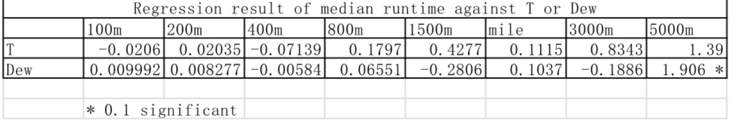
For each event, median running time on each date is calculated. Regression analysis of median running time of some date against temperature and against dew point on that date is performed. Table 3 shows the results of simple linear regression and Figure 4 displays the scatterplots of median running time against T and against Dew for selected events. The models used in Table 2 are lm(median runtime ~ T) and lm(median runtime ~ Dew).
Table 2: regression coefficients for each event with significant level
100m 200m 400m 800m 1500m mile 3000m 5000m
T -0.0206 0.02035 -0.07139 0.1797 0.4277 0.1115 0.8343 1.39
Dew 0.009992 0.008277 -0.00584 0.06551 -0.2806 0.1037 -0.1886 1.906 *
* 0.1 significant
Figure 2: scatterplot of median runtime against T and against Dew
The table and figure above show that simple linear regression does not model the
relationship between weather factors and running performance well. Almost all the regression coefficients are not significant (except for Dew Point in 5000m event), which suggests that we need more sophisticated modeling method than simple linear regression. One possible model is the general mixed model, which will be presented in the following sections.
Methodology
In this paper, I analyze the data using the following models: (1) lm1
log(𝑡𝑖𝑗𝑘) = 𝛼𝑖+𝛽𝑇∗ 𝑇𝑗𝑘+ 𝛽𝐷𝑒𝑤∗ 𝐷𝑒𝑤𝑗𝑘+ 𝑆(𝑎𝑖𝑗) + 𝜖𝑖𝑗𝑘
(2) lm2
log(𝑡𝑖𝑗𝑘) = 𝛼𝑖+ 𝛽𝑇∗ 𝑇𝑗𝑘+ 𝛽𝐷𝑒𝑤∗ 𝐷𝑒𝑤𝑗𝑘+ 𝛽𝑖𝑛𝑡𝑒𝑟𝑎𝑐𝑡𝑖𝑜𝑛∗ 𝑇𝑗𝑘∗ 𝐷𝑒𝑤𝑗𝑘+ 𝑆(𝑎𝑖𝑗) + 𝜖𝑖𝑗𝑘
(3) lm3
(4) lm4
log(𝑡𝑖𝑗𝑘) = 𝛼𝑖+ 𝛽𝐷𝑒𝑤∗ 𝐷𝑒𝑤𝑗𝑘+ 𝑆(𝑎𝑖𝑗) + 𝜖𝑖𝑗𝑘
where
𝑡𝑖𝑗𝑘 is the finish time of runner 𝑖 on date 𝑗 for event 𝑘, 𝛼𝑖 is a constant representing the overall ability of runner 𝑖, 𝛽𝑇 is the coefficient representing the effect of temperature, 𝛽𝐷𝑒𝑤 is the coefficient representing the effect of Dew point,
𝛽𝑖𝑛𝑡𝑒𝑟𝑎𝑐𝑡𝑖𝑜𝑛 is the coefficient of interaction of temperature and Dew point, 𝑇𝑗𝑘 is the temperature of date 𝑗 for event 𝑘,
𝐷𝑒𝑤𝑗𝑘 is the Dew point of date 𝑗 for event 𝑘, 𝑎𝑖𝑗 is the age of runner 𝑖 on date 𝑗,
𝑆(𝑎𝑖𝑗) is the polynomial term representing age effect; it can be linear, quadratic, or zero (when using age_index.csv, meaning that age effect is already included in the individual effect),
𝜖𝑖𝑗𝑘 is the random error.
Model (5), (6), (7), and (8) are the same as above except that log(𝑡𝑖𝑗𝑘) is replaced by
(𝑡𝑖𝑗𝑘)
There are 8 events in total: 100m, 200m, 400m, 800m, 1500m, mile, 3000m, and 5000m. We believe weather effects are different for each event, and so separate statistical analysis is performed for each event. The eight models above are selected based on the number of significant coefficients. Quadratic T and Dew terms have also been tried in the models but they did not show significant results.
levels. The difference between the mixed model and the simple linear model is that in the simple linear model, we define things we can control as explanatory variables and define error as all other effects that we do not understand or are not interested in. In the mixed model, however, the random effects give structure to the error term and enable us to better study them. In this research project, the fixed effects are temperature, Dew point and age because they are measurable variables and we want to study how they affect track performance. Random effects are the unobserved idiosyncratic variation that is due to differences among individuals. We treat individual effects as random effects because we expect running performance within each individual to be correlated. Reasons for this may be that runners have preferences on which event to participate and runners have widely different running abilities.
Model (2) uses the interaction term of temperature and Dew point because it is reasonable to assume that heat and humidity have a combined effect on running performance. A study performed by Professor Mureika of the Physics Department of Loyola Marymount University suggests that the combined effect of relative humidity and temperature plays a crucial role in adjusting running performances in 100m races, since the air density of hot, saturated air is significantly lower than that of colder, dry air (Mureika, 2014).
Age is included in all regression models because the data cover 11 years and as many runners participated over multiple years, their performances are influenced by their increasing ages. In this study, we examined three possible ways to model age: simple linear regression on age, quadratic regression on age+age^2 and not including age in the model (when using age_index.csv as dataset). Quadratic regression suits better for longer-term events because we observe that the relationship between age and media runtime performance tends to be more quadratic than linear for events longer than 1500m.
The use of log(𝑡𝑖𝑗𝑘) rather than 𝑡𝑖𝑗𝑘 is appropriate here because marginal changes in
finish time and finish time, regression analysis is performed using both.
Results and discussion
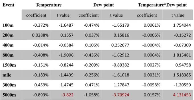
Originally, I used the full running performance data from 2002 to 2014. However, the regression results based on the full dataset do not show much statistical significance (details shown in Table 3), potentially because there are outliers in running performance in some years. Therefore, we omit one year in the dataset and run mixed model regression on the new dataset and find out that the optimal dataset, defined as the model with most number of significant coefficient, is the one from 2003 to 2013. The following discussions are based on the results from 2003 to 2013.
Event Temperature Dew point Temperature*Dew point
coefficient t value coefficient t value coefficient t value 100m -0.372% -1.6487 -0.474% -1.65179 0.0061% 1.754044
200m 0.0288% 0.1557 0.037% 0.15816 -0.0005% -0.15272
400m -0.014% -0.0384 0.106% 0.252677 -0.0004% -0.07309
800m -0.408% -1.9006 -0.436% -1.62912 0.0064% 1.815481
1500m -0.151% -0.8244 -0.209% -0.89382 0.0027% 0.94758
mile -0.183% -1.4439 -0.256% -1.61018 0.0031% 1.518385
3000m 0.459% 1.4745 0.471% 1.27847 -0.0058% -1.20559
5000m -0.893% -3.822 -1.058% -3.70924 0.0157% 4.131453
Table 3: regression results for lm2 using data 2002 ~ 2014, with log runtime (red cell indicates significant coefficient under 95% confidence)
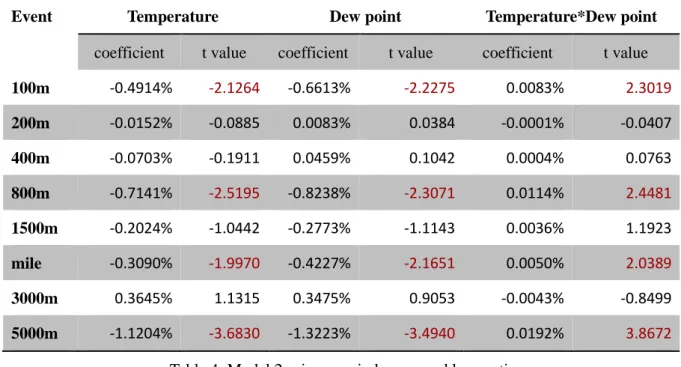
Event Temperature Dew point Temperature*Dew point
coefficient t value coefficient t value coefficient t value 100m -0.4914% -2.1264 -0.6613% -2.2275 0.0083% 2.3019
200m -0.0152% -0.0885 0.0083% 0.0384 -0.0001% -0.0407
400m -0.0703% -0.1911 0.0459% 0.1042 0.0004% 0.0763
800m -0.7141% -2.5195 -0.8238% -2.3071 0.0114% 2.4481
1500m -0.2024% -1.0442 -0.2773% -1.1143 0.0036% 1.1923
mile -0.3090% -1.9970 -0.4227% -2.1651 0.0050% 2.0389
3000m 0.3645% 1.1315 0.3475% 0.9053 -0.0043% -0.8499
5000m -1.1204% -3.6830 -1.3223% -3.4940 0.0192% 3.8672
Table 4: Model 2 using age_index.csv and log runtime
Figure 3: Coefficient Comparison of lm2, lm3 and lm4 using data from 2003 to 2013
Figure 3 shows the results of 3 regression models using dataset age_index.csv: linear regression on T (lm3), linear regression of Dew (lm4), linear regression T, Dew and interaction term T*Dew (lm2). As we can see from the graph, the coefficient for the
-0.0005 0 0.0005 0.001 0.0015 0.002 0.0025 0.003
100m 200m 400m 800m 1500m mile 3000m 5000m
Result Comparison of lm2, lm3, lm4
interaction term is closest to zero. The coefficients for T and Dew respectively are higher and tend to increase as the event distance increases. Interpreting the coefficient in lm3 and lm4 are straightforward. For instance, Model 3 gives us a coefficient on T of 0.00101185 for 3000m event. This indicates that in 3000m race, a unit increase in temperature improves running performance by 0.101%. Note that this is a very small number, which implies that temperature alone may not have a strong effect on running performance.
Adding an interaction term in our model drastically changes the interpretation of all the coefficients. Coefficient of T is now interpreted as the effect of temperature on log finish time only when Dew = 0. Similarly, coefficient of Dew is the effect of Dew point on log finish time only when T = 0. Since temperature and Dew point are both continuous variable and are unlikely to be 0 in reality, it is less important to look at their coefficients. What is more important is the coefficient of the interaction term, which can interpreted as the effect of temperature on log finish time for different levels of Dew point, or the effect of Dew point for different levels of temperature. A positive interaction coefficient means that a unit increase in Dew point leads to an increase in the marginal effect of temperature on finish time. For instance, in 5000m event the interaction coefficient is 0.019%. This indicates that as Dew point increases 1 unit, the marginal effect of temperature on finish time is increased by 0.019%.
Since lmer function does not produce p value or degree of freedom in the output and instead shows t value, we use a general rule of thumb that t value greater than or equal to 1.96 indicates a significant coefficient (p value < 0.05). This is based on the assumption that t distribution converges to z distribution as degrees of freedom increase. For Model 3 and Model 4, the coefficients are only significant for event 3000m and 5000m. For the interaction term (Model 2) in the regression analysis, its coefficient is significant in 100m, 800m, mile and 5000m running events and not significant in the other events. Since the null hypothesis of the regression is that coefficients of explanatory variables equal to zero, whether significant or not in the case suggests temperature and dew point have no effect on running performance for 200m, 400, 1500m and 3000m events.
200m event. Taking a further look at the results in lm3 and lm4 for 3000m and 5000m, we noticed that the coefficients for temperature are positive for both events, indicating that when temperature or dew point increases, running performance is worsened. Such results align with the intuition that in long-distance running events, athletes usually have a problem with hot or humid weather. The model did not find significant weather effect on running performance in short-distance events.
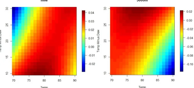
If we look at the significant coefficients in lm2, though, the model gives us very different results. The coefficients of temperature and dew point in 100m, 800m, mile and 5000m events are all negative. The coefficients of temperature and dew point’s interaction term in 100m, 800m, mile and 5000m events are all positive. Because of the interaction term, it is difficult to interpret coefficients directly. To better interpret the results of model 2, I plotted the heat map, with temperature on the x-axis, temperature minus dew point on the y-axis and 𝑧 = (𝛽𝑇∗ 𝑇𝑗𝑘+ 𝛽𝐷𝑒𝑤∗ 𝐷𝑒𝑤𝑗𝑘+ 𝛽𝑖𝑛𝑡𝑒𝑟𝑎𝑐𝑡𝑖𝑜𝑛∗ 𝑇𝑗𝑘∗ 𝐷𝑒𝑤𝑗𝑘)/(𝛽𝑇∗ 70+ 𝛽𝐷𝑒𝑤∗ 50 + 𝛽𝑖𝑛𝑡𝑒𝑟𝑎𝑐𝑡𝑖𝑜𝑛∗
Figure 4: Heat Map of 100m, 800m, mile and 5000m using lm2 results
The heat map of 100m shows that if temperature is low in the 70s, the wider the difference between dew point and temperature, the more improvement in running performance. On the contrary, if temperature is high in the 90s, the wider the difference between dew point and temperature, the worse the running performance is. Similarly, the heat map of 800m and 5000m events both indicate that when temperature is high, the closer temperature and dew point are, the better running performance is. The heat map of mile events, however, shows that when temperature is low in the 70s, the wider the wider the difference between dew point and temperature, the better the running performance is. The heat maps give me very mixed interpretations. The results for 5000m and 800m are somehow counter-intuitive whereas the results for mile fall into my expectation. Because model 2 is only significant for these four events, it is difficult to trust the interpretation. More complicated models may be needed to describe the relationship between weather and running performance more accurately.
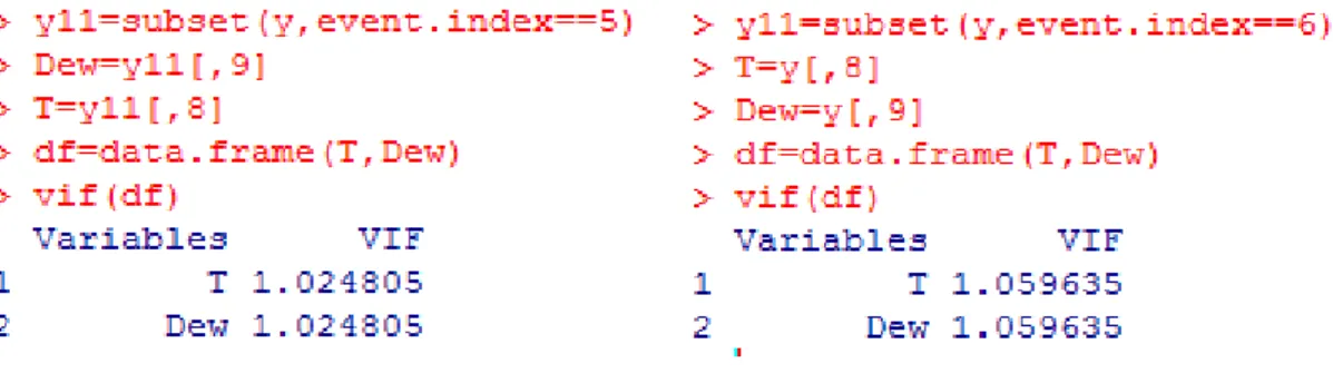
explanatory variables. Therefore, other reasons need to be discovered. Figure 5 presents a detailed result.
Figure 5: Collinearity test for 1500m event and 3000m event
Linear and quadratic age models are also tested in R but they do not generate much significant coefficient. Thus, we choose to use age_index.csv dataset, which incorporates age effect in the individual effect.
In addition, in 5000m event, the coefficient for T, Dew, T*Dew and the quadratic terms of T and Dew are all significant, implying that the result for 5000m event is robust.
Conclusion
While temperature and Dew point by themselves only have a significant effect on running performance in 3000m and 5000m events, the combined effect of temperature and Dew point have significant effect on more events, including 100m, 800m, mile, and 5000m. We can draw the preliminary conclusion that in long-distance events, hot and humid weather slows down the running performance. However, to model the weather effect more accurately, more sophisticated models need to be used and tested.
Further Consideration
Appendix
1. R code
y=read.csv('final_dataset_04082015_age_index.csv') output=matrix(nrow=28,ncol=8)
for (i in 1:8) {
output[16,i]=result5[6,3] output[17,i]=result5[4,1] output[18,i]=result5[4,3] output[19,i]=result5[5,1] output[20,i]=result5[5,3]
lm3=lmer(formula=logtime~T+(1|runner.index)) result3=data.frame(coef(summary(lm3))) output[21,i]=result3[2,1]
output[22,i]=result3[2,3]
lm4=lmer(formula=logtime~Dew+(1|runner.index)) result4=data.frame(coef(summary(lm4)))
output[23,i]=result4[2,1] output[24,i]=result4[2,3]
}
write.table(output,file="output.csv")
2. Compilation of Regression results Models tested:
(1) lm1
log(𝑡𝑖𝑗𝑘) = 𝛼𝑖+𝛽𝑇∗ 𝑇𝑗𝑘+ 𝛽𝐷𝑒𝑤∗ 𝐷𝑒𝑤𝑗𝑘+ 𝑆(𝑎𝑖𝑗) + 𝜖𝑖𝑗𝑘
(2) lm2
log(𝑡𝑖𝑗𝑘) = 𝛼𝑖+ 𝛽𝑇∗ 𝑇𝑗𝑘+ 𝛽𝐷𝑒𝑤∗ 𝐷𝑒𝑤𝑗𝑘+ 𝛽𝑖𝑛𝑡𝑒𝑟𝑎𝑐𝑡𝑖𝑜𝑛∗ 𝑇𝑗𝑘∗ 𝐷𝑒𝑤𝑗𝑘+ 𝑆(𝑎𝑖𝑗) + 𝜖𝑖𝑗𝑘
(3) lm3
log(𝑡𝑖𝑗𝑘) = 𝛼𝑖+ 𝛽𝑇∗ 𝑇𝑗𝑘+ 𝑆(𝑎𝑖𝑗) + 𝜖𝑖𝑗𝑘
(4) lm4
log(𝑡𝑖𝑗𝑘) = 𝛼𝑖+ 𝛽𝐷𝑒𝑤∗ 𝐷𝑒𝑤𝑗𝑘+ 𝑆(𝑎𝑖𝑗) + 𝜖𝑖𝑗𝑘
where
𝛽𝐷𝑒𝑤 is the coefficient representing the effect of Dew point,
𝛽𝑖𝑛𝑡𝑒𝑟𝑎𝑐𝑡𝑖𝑜𝑛 is the coefficient of interaction of temperature and Dew point, 𝑇𝑗𝑘 is the temperature of date 𝑗 for event 𝑘,
𝐷𝑒𝑤𝑗𝑘 is the Dew point of date 𝑗 for event 𝑘, 𝑎𝑖𝑗 is the age of runner 𝑖 on date 𝑗,
𝑆(𝑎𝑖𝑗) is the polynomial term representing age effect; it can be linear, quadratic, or zero (when using age_index.csv, meaning that age effect is already included in the individual effect),
𝜖𝑖𝑗𝑘 is the random error.
Model (5), (6), (7), and (8) are the same as above except that log(𝑡𝑖𝑗𝑘) is replaced by (𝑡𝑖𝑗𝑘)
3. Detailed regression results
Using logtime; significant terms are marked in red
lm1=lmer(formula=logtime~T+Dew+(1|runner.index))
lm2=lmer(formula=logtime~T+Dew+T*Dew+(1|runner.index)) lm3=lmer(formula=logtime~T+(1|runner.index))
lm4=lmer(formula=logtime~Dew+(1|runner.index))
100m 200m 400m 800m 1500m mile 3000m 5000m
lm1_coef_T 0.000376 -0.000221 -0.000424 -0.000239 0.000275 0.000045 0.000919 0.000498
lm1_tvalue_T 1.556492 -1.174305 -1.185287 -0.819489 1.400457 0.263716 2.992738 1.595196 lm1_coef_Dew 0.000198 -0.000005 0.000794 0.000471 0.000185 -0.000266 0.000223 0.001347 lm1_tvalue_Dew 0.822375 -0.021429 2.224743 1.525322 0.966811 -1.383149 0.742286 3.722250
lm2_coef_T -0.004914 -0.000152 -0.000703 -0.007141 -0.002024 -0.003090 0.003645 -0.011204 lm2_tvalue_T -2.126435 -0.088488 -0.191083 -2.519549 -1.044211 -1.996963 1.131487 -3.682965
lm2_coef_Dew -0.006613 0.000083 0.000459 -0.008238 -0.002773 -0.004227 0.003475 -0.013223 lm2_tvalue_Dew -2.227492 0.038371 0.104173 -2.307138 -1.114325 -2.165145 0.905297 -3.493960
lm2_coef_T*Dew 0.000083 -0.000001 0.000004 0.000114 0.000036 0.000050 -0.000043 0.000192 lm2_tavlue_T*Dew 2.301914 -0.040738 0.076330 2.448130 1.192257 2.038947 -0.849926 3.867222
lm3_coef_T 0.000411 -0.000222 -0.000098 -0.000053 0.000312 -0.000005 0.001012 0.001032 lm3_tvalue_T 1.725227 -1.194798 -0.301415 -0.200539 1.619938 -0.027832 3.601952 3.710499
Using runtime; significant terms are marked in red
lm1=lmer(formula=runtime~T+Dew+(1|runner.index))
lm2=lmer(formula=runtime~T+Dew+T*Dew+(1|runner.index)) lm3=lmer(formula=runtime~T+(1|runner.index))
lm4=lmer(formula=runtime~Dew+(1|runner.index))
100m 200m 400m 800m 1500m mile 3000m 5000m
lm1_coef_T 0.008952 -0.009174 -0.047218 -0.036263 0.111097 0.009835 0.853398 0.670256
lm1_tvalue_T 1.851335 -1.169775 -0.889392 -0.618520 1.400735 0.135228 3.162593 1.478598
lm1_coef_Dew 0.005072 0.000826 0.131034 0.093254 0.077818 -0.106088 0.169328 1.940586
lm1_tvalue_Dew 1.050849 0.091629 2.441345 1.503641 1.005745 -1.309321 0.642466 3.692070
lm2_coef_T -0.105196 -0.013494 0.586018 -1.452474 -0.710855 -1.228083 3.872469 -16.378596 lm2_tvalue_T -2.271618 -0.189354 1.066886 -2.550392 -0.907484 -1.880633 1.368875 -3.705604
lm2_coef_Dew -0.141968 -0.004627 0.890716 -1.693494 -0.979640 -1.670312 3.772154 -19.288158 lm2_tvalue_Dew -2.385161 -0.051518 1.353566 -2.360598 -0.974264 -2.027025 1.118981 -3.507810
lm2_coef_T*Dew 0.001795 0.000069 -0.009857 0.023295 0.012949 0.019875 -0.047095 0.279803 lm2_tavlue_T*Dew 2.478484 0.061008 -1.158291 2.499930 1.054776 1.907491 -1.072072 3.877995
lm3_coef_T 0.009827 -0.009056 0.003633 0.000511 0.126626 -0.010187 0.923589 1.439846
lm3_tvalue_T 2.063219 -1.171104 0.074302 0.009587 1.627553 -0.143238 3.742708 3.559769
References
"Running in Heat and Humidity." Running in Heat and Humidity. Over40runner, n.d. Web. 06 Dec. 2014.
Mureika, J. R. "The Effects of Temperature, Pressure, and Humidity Variations on 100 Meter Sprint Performances." (n.d.). 06 Dec. 2014. Web.
Nour El Helou, Muriel Ta_et, Geo_roy Berthelot, Julien Tolaini, Andy Marc, Marion Guillaume, Christophe Hausswirth, Jean-Fran_cois Toussaint (2012), Impact of
Environmental Parameters on Marathon Running Performance. PLoS ONE, Volume 7, Issue 5, paper e37407, 1 May 2012.
Williams, Richard. "Panel Data 4: Fixed Effects vs Random Effects Models." (n.d.). Web. 8 Dec. 2014.
Mortimer, Jeylan T., and Michael J. Shanahan. "Panel Models for the Analysis of Change and Growth in Life Course Studies." Handbook of the Life Course. New York: Kluwer Academic/Plenum, 2003. 510-11. Print.
Pfitzinger, Pete. "Hydration and Heat Management." Runner's World & Running Times. July 2006. Web. 16 Apr. 2015.
Barry, Kristin. "Weather Your Summer Workouts" Runner's World & Running Times. July 2011. Web. 16 Apr. 2015.
"MPR - Training Paces." MPR - Training Paces. MPR Coaching Services,
http://www.mprunning.com/training_paces.html. n.d. Web. 16 Apr. 2015.
Acknowledgement