2 ACKNOWLEDGEMENTS:
I would like to thank my committee for their continued support and commitment to my success. A very special thank you goes to Amanda Dye for her invaluable support with the day-to-day tasks of this study. I would also like to thank others who contributed to the success of this study: Dr. James McClure, Morgan Talley, and Blythe Carter.
This work was supported by:
National Science Foundation Grant 0941235 Department of Energy Grant DE-SC0002163,
National Institute of Environmental Health Sciences Grant P42 ES05948.
3 TABLE OF CONTENTS:
List of Tables ………..4
List of Figures ……….4
Abstract………....5
Introduction……….5
Materials and Methods………7
Results ………12
Discussion………...…24
4 LIST OF TABLES
Table 1. Number of DNRs observed relative to total number of DNRs.
Table 2. Average SSACR and orientation in flow for aggregate DNR system throughout dissolution.
Table 3. Average volume, surface areas and parameterized surface areas for aggregate DNR system throughout dissolution.
Table 4. Morphological characteristic of Reeves throughout dissolution.
Table 5. Morphological characteristic of Ian throughout dissolution.
Table 6. Volume, SSACR, surface areas and parameterized surface areas for DNRs in the Remain and Dissolve groups.
LIST OF FIGURES
Figure 1. Visualized X-ray transmission values for a cross-section of the column using beam energies above the cesium K-edge (a), between the iodine K-edge and the cesium K- edge (b) and below the iodine K-edge (c).
Figure 2. Histograms of mesh (X-ray transmission) values associated with using beam energies above the cesium K-edge (a), between the iodine K-edge and the cesium K-edge (b) and below the iodine K-edge (c).
Figure 3. Individual and median volume throughout dissolution of DNRs that remained in the second dissolution step.
Figure 4. Individual and median DNR SSACR throughout dissolution for DNRs that remained in the second dissolution step
Figure 5. Wetting-nonwetting intrinsic surface area of DNRs that remained after two dissolution steps
5 ABSTRACT:
Organic immiscible fluids are common subsurface contaminants which may leach into
the groundwater supply, posing a threat to human health. The development of effective
remediation techniques is dependent upon a thorough understanding of the microscale processes
that govern the dissolution of non-aqueous phase liquid (NAPL). In order to resolve the local
mass transfer in the dissolution process from a fundamental perspective, both the pore-space and
NAPL morphology must be known. The purpose of this study was to assess the morphology of
trapped NAPL during dissolution using three-dimensional (3-D) image analysis. Data was taken
from a previous experiment where a column was packed with a representative porous medium
and trichloroethylene (TCE), and flushed with a solution containing
hydroxypropyl-β-cyclodextrin (Schnaar and Brusseau 2006). 3-D images were taken of the column in its residual
state and after each successive flush using X-ray microtomography. Image analysis was
performed to assess the orientation, curvature, volume, and surface area of the NAPL. A
comparison was constructed between the disconnected NAPL regions (DNRs) that were flushed
and those that persisted. The volume, roundedness and orientation were important determinants
of dissolution.
INTRODUCTION:
NAPLs including chlorinated solvents, fuel oils and gasoline products are common
subsurface contaminants. These compounds, often released into the environment by industrial
processes, may become trapped in the subsurface due to capillary forces. Trapped NAPLs slowly
dissolve over time, creating a long-term source of pollution for the drinking water supply. Many
6
carcinogens. As such, their presence in the drinking water supply is a significant threat to human
health.
To assess the risk posed by trapped NAPL to groundwater resources, its dissolution
behavior must be understood. In the microscale, dissolution is governed by the mass transfer
between the NAPL and the aqueous phase. Models commonly characterize the mass transfer
between the non-aqueous and aqueous phases as being proportional to the product of the
deviation of the aqueous phase concentration of the dissolved NAPL from equilibrium (Miller et.
al 1990). However, accurate representations of NAPL morphology and the NAPL-aqueous
interface are typically not accessible quantities (Khachikian and Harmon 2000). By
constructing a better understanding of trapped NAPL morphology, the ability to predict NAPL
dissolution will be improved.
There have been numerous previous attempts to characterize NAPL morphology during
dissolution. Early studies relied on styrene polymerization of NAPL bodies to quantify their
shape and size (e.g. Powers et. al. 1994). The inherent disadvantage of this study design is that it
is invasive; each phase is separated to recover the polymerized NAPL. This feature makes it
difficult to assess changes to NAPL throughout the dissolution process (Khachikian and Harmon
2000). Other studies have relied on two-dimensional micromodels to characterize NAPL
morphology (e.g. Corapcioglu et. al. 2009). These studies assess the behavior of NAPL within
an artificial, transparent network of interconnecting pores and throats (Corapcioglu et. al. 2009).
Advances in 3-D imaging technologies have furthered our ability to study NAPL
dissolution. The non-invasive nature of 3-D imaging allows for the assessment of changes to the
morphology of an individual NAPL region (DNR) throughout dissolution. Previous studies have
7
area-to-volume ratio (Johns and Gladden 2000). However, due to limitations in resolving the
phases within the image taken by MRI, the study used 1mm ballotini as the representative porous
media, where the grain size of natural soils ranges from 0.25 mm to 1.0 mm (Johns and Gladden
2001). Another study, conducted by Zhang et. al. used synchrotron X-ray microtomography to
directly quantify NAPL size and geometry (2002). However, due to poor resolution, the study
was unable to identify DNRs in isolation; instead, investigators relied on integrated measures of
all DNRs within their experiment (Zhang et. al. 2002).
The current study uses images taken from a previous study performed by Schnaar and
Brusseau (2006). The current study resolved the images and analyzed them for the following
parameters: volume, curvature, orientation, and interfacial surface area.
MATERIALS AND METHODS
TCE was used as the model NAPL for this study. The TCE was doped with iodobenzene
(8% by volume) to enhance image contrast. The aqueous phase was doped with cesium chloride
(60 g/L). Commercially available 45/50 Accusand (Accusand, Unimin Co.) was used as the
representative porous medium. The median grain size of the media was 0.35mm. The uniformity
coefficient (U = d60/d10; di is the ith percentile of grains by mass that are smaller than a given
sieve size) of the media was 1.0.
Establishment of Organic-Liquid Saturation and Column Flushing
As described by Schnaar and Brusseau (2006), the porous medium was dry-packed into a
thin-walled, X-ray transparent column made of aluminum, with Swagelok end-fittings. The
column was 4.4 cm long, with an inner diameter of 0.58 cm. Glass inserts (1.4 cm long, 0.2 cm
in diameter) were placed at the ends of the column. Polypropylene frits (10-μm pores) were
8
length of the porous medium zone was approximately 1.5 cm. The equivalent of 5 pore-volumes
( 1 cm3) of TCE was then pumped vertically upward into the column using a syringe pump
(Sage). An aqueous solution containing TCE and iodobenzene was then flushed vertically
downward at 20 cm/hr to displace the organic liquid.
As discussed by Schnaar and Brusseau (2006), the column was then sealed and imaged as
described below. After the first, “residual” scan, the column was flushed with an aqueous
solution at a Darcy velocity of 17 cm/hr. To increase the solubility of the organic liquid in the
aqueous phase, the flushing solution contained hydroxypropyl-β-cyclodextrin (HPCD, 5 wt %).
During each dissolution step, approximately 65 pore volumes of the HPCD solution were
flushed through the column. Following this, approximately 10 additional pore volumes of
solution containing no HPCD and 60 g/L cesium chloride were flushed through the column to
introduce the aqueous-phase dopant. The column flushing procedure was implemented three
times on the column. The column was sealed and imaged following each dissolution step.
Synchrotron X-ray micro-tomography
3-D images were taken of the column in its residual state and after each dissolution step.
Imaging was performed at the GeoSoilEnviroCARS BM-13D Beamline at the Advanced Photon
Source at Argonne National Laboratory, Illinois. The imaged zone spanned the entire length of
the porous medium zone within the column. Two beams of different energies were used to
resolve each of the three phases. Images were collected above and below the iodine K-edge
(33.0169 and 33.269 keV) to resolve the non-aqueous phase, and below and above the cesium
K-edge (33.279 and 36.085 keV) to resolve the aqueous phase. Spatial resolution of the images
9 Resolving the image and data processing
The raw data from the imaging process consisted of three, 3-D meshes, with each mesh
corresponding to one of the energy levels used in the X-ray micro-tomography: below the iodine
K-edge, between the iodine K-edge and the cesium K-edge and above the cesium K-edge. Mesh
values were the X-ray transmission for a given point within the column. Cross-sections of the
10
(a)
(b)
(c)
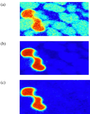
Figure 1. Visualized X-ray transmission values for a cross-section of the column using beam energies above the cesium K-edge (a), between the iodine K-edge and the cesium K-edge (b) and below the iodine K-edge (c).
The goal of image processing was to construct a composite image from the three meshes
where the solid, non-aqueous and aqueous phases were each well-resolved. The raw image
constructed by the meshes yielded poor separation between the phases, making it difficult to
identify interfaces (Figure 1). The meshes were processed to enhance the resolution of the
phases, and thus enable the study of interfacial area. First, the meshes were subjected to a
modified Gaussian filtering algorithm to remove noise from the histogram of X-ray transmission
values. Each phase was assumed to have a normal distribution. For transmission values that
were located within overlapping phase distributions, the probability of transmission value
X-11
ray transmission values associated with each interface was identified. Figure 2 shows a
histogram of the X-ray transmission values for the mesh for each energy beam used during
micro-tomography. The greatest, middle and smallest peaks of the histogram correspond to the
X-ray transmission values associated with the solid, aqueous and non-aqueous phases,
respectively (Figure 2). An isovalue mask was applied to the mesh and the enclosed area was
cropped. The value of the mask was chosen to be the average transmission between the peaks on
the histogram. This value is the transmission level associated with the interface between any two
12
(a)
(b)
(c)
Figure 2. Histograms of mesh (X-ray transmission) values associated with using beam energies above the cesium K-edge (a), between the iodine K-edge and the cesium K-edge (b) and below the iodine K-edge (c).
Once the interfaces were rendered sufficiently smooth, the images were analyzed using
the image processing software DataTank, which is available online from
http://www.visualdatatools.com/DataTank/index.html. DataTank assessed the NAPL for the
13
will rely on terminology commonly used in describing multiphase flow. The NAPL may
hereafter be referred to as the nonwetting (N) phase, the aqueous solution may be described as
the wetting (W) phase, and the solid may be referred to as the solid (S) phase
DNR orientation was quantified by the orientation tensor. At each point on the interface,
the orientation was calculated as the dyadic product of the normal vector. These values were then
averaged over both the nonwetting-wetting (NW) and nonwetting-solid (NS) interfaces to
generate the reported values. This analysis focuses on the Gzz value for the NW interface, as it
was observed to have the greatest changes throughout dissolution, and the aqueous solution was
flushed in the vertical, z-direction.
It was hypothesized that the DNR would become more rounded throughout dissolution.
This morphological change was quantified by the unitless parameter of the specific surface
area-to-curvature ratio (SSACR). By comparing the SSACR of a given DNR to the SSACR of a
sphere, one can deduce the overall roundedness of a NAPL feature. The curvature, J, was
calculated as the divergence of the normal vector at a given point (m-1). This value was averaged
over the entire DNR surface, generating an average curvature. The specific surface area (SSA)
was calculated as the surface area to volume ratio (m2m-3). These values are defined
mathematically as follows:
For a sphere, J can be simplified to
14
Finally, the SSACR is the ratio of the SSA to the curvature is equal to
Thus, the overall roundedness of a DNR can be quantified by comparing its SSACR to
that of a sphere, or 1.5. The final value used in this analysis is the specific interfacial area (SIA),
or the ratio of the surface area of the NW interface to the total volume. This value describes the
contact of each DNR with the wetting fluid relative to its total volume.
RESULTS
This results section consists of three types of analysis. First, the aggregate system of all
DNRs is assessed throughout each dissolution step. Second, the DNRs that remained after two
dissolution steps are examined to assess changes to their morphology throughout dissolution.
Finally, a comparison was constructed between DNRs that dissolved and DNRs that remained
entrapped. This comparison allows for the identification of morphological characteristics shared
by DNRs that are dissolved.
Aggregate System
The DNRs observed in this study were a subset of all DNRs in the column (Table 1).
Some of the DNRs were in contact with the column wall and are considered separately for
portions of this analysis. Contact with the column wall may influence the dissolution behavior,
and thus, DNRs located on the column wall may not be representative of NAPL within a natural
15
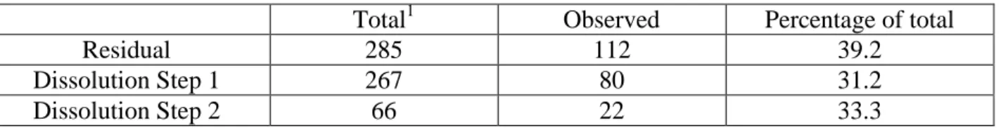
Table 1. Number of DNRs observed relative to total number of DNRs
Total1 Observed Percentage of total
Residual 285 112 39.2
Dissolution Step 1 267 80 31.2
Dissolution Step 2 66 22 33.3
Changes to the average orientation of the interface in the direction of flow, the NW Gzz,
were observed. The NW interface tended to be less oriented in the direction of flow for the
residual and the second dissolution step, but more oriented in the direction of flow for the first
dissolution step (Table 2). While the NW interface for DNRs along the column wall tended to be
more oriented in the direction of flow, they observed the same trend as the interior DNRs.
NAPL SSACR increased during each dissolution step.
Table 2. SSACR and NW Gzz for aggregate DNR system throughout dissolution.
Residual Dissolution Step 1 Dissolution Step 2
SSACR 1.96 5.85 6.84
On wall 2.14 6.94 7.03
Interior 1.81 4.25 6.73
NW Gzz 0.289 0.311 0.267
On wall 0.298 0.320 0.277
Interior 0.277 0.299 0.262
The average volume of the DNRs decreased between the residual and the first dissolution
step, but increased between the first and second dissolution steps (Table 3). The DNRs on the
column wall had a larger average volume than the DNRs on the interior, but followed the same
trend. The average NW interfacial area increased throughout dissolution, while the average NS
interfacial area decreased slightly in the first dissolution step and increased in the second
dissolution step (Table 3). SIA increased throughout dissolution (Table 3).
1
16
Table 3. Average volume, surface areas and parameterized surface areas for aggregate DNR system throughout dissolution.
Residual Dissolution Step 1 Dissolution Step 2
Volume (m3) 6.48E-11 5.50E-11 7.88E-11
On wall 7.33E-11 6.00E-11 1.40E-10
Interior 5.22E-11 4.75E-11 5.02E-11
NW Interfacial Area (m2) 6.28-08 1.32E-07 2.40E-07
On wall 6.45E-08 1.32E-07 4.55E-07
Interior 6.04E-08 1.31E-07 1.39E-07
NS Interfacial Area (m2) 7.80E-07 5.34E-07 5.38E-07
On wall 7.79E-07 4.79E-07 7.35E-07
Interior 7.82E-07 6.17E-07 4.47E-07
SIA (m-1) 9.70E2 2.40E3 3.04E3
On wall 8.80E2 2.20E3 3.25E3
Interior 1.16E3 2.77E3 2.77E3
Changes to individual DNR morphology throughout dissolution
Changes in the morphology of an individual DNR throughout dissolution were assessed.
In this section, DNRs may be referred to by their identifying handle. Of the 112 DNRs selected
in the residual, 19 remained after the second dissolution step. Two DNRs, Reeves and Apollo,
were partially dissolved during the second dissolution step, breaking into smaller DNRs. These
DNRs were assessed as independent features, denoted by Roman numerals (e.g. Apollo I, Apollo
II). From the 19 parent DNRs and 3 newly isolated DNRs from Reeves and Apollo, there were a
total of 22 DNRs assessed in this section.
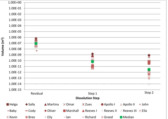
DNRs tended to decrease in volume throughout dissolution. Figure 3 displays the
volume for individual DNR during the three dissolution steps. Additionally, the median DNR
volume is shown, indicating the general trend of decreasing volume. DNR volume decreased
more dramatically between the first and second dissolution steps. Volume had a greater variance
17
Figure 3. Individual and median volume throughout dissolution for DNRs that remained in the second dissolution step.
The overall roundedness of a DNR, the SSACR was assessed during each dissolution
step. SSACR generally increased throughout dissolution, deviating from the SSACR of a sphere.
Figure 4 illustrates the changes observed in each DNR, as well as the median value. 1.00E-15 1.00E-14 1.00E-13 1.00E-12 1.00E-11 1.00E-10 1.00E-09 1.00E-08 1.00E-07 1.00E-06 1.00E-05 1.00E-04 1.00E-03 1.00E-02 1.00E-01 1.00E+00 Vo lu m e (m 3) Dissolution Step
Helga Sally Martina Omar Zues Apollo I Apollo II John
Baby Cody Oliver Marshall Reeves I Reeves II Reeves III Ella
Kevin Bree Eily Ian Richard Greed Median
18
Figure 4. Individual and median SSACR throughout dissolution for DNRs that remained in the second dissolution step.
Generally, SIA increased throughout dissolution, but an increased variance was also
observed (Figure 5). To explore this notion, two DNRs, Reeves and Ian, will be examined as
19
Figure 5. SIA dissolution of the DNRs that remained after two dissolution steps2
Reeves was a large DNR located on the column wall. Morphological characteristics for
Reeves are summarized in Table 4. In the first dissolution step, the volume decreased as a large
lobe of the DNR was dissolved. In the second dissolution step, Reeves was almost entirely
dissolved, leaving three small, isolated features (Reeves I, Reeves II and Reeves III). Reeves
exhibited an increase in SIA between the residual and first dissolution step and a dramatic
increase in SIA was observed between the first and second dissolution steps. Reeves’s SSACR
increased throughout dissolution.
2
A small DNR, Belle, was excluded from this analysis because it had zero NW interfacial area during all three dissolution steps. 1 10 100 1000 10000 100000 1000000 10000000 SIA ( m
2 m -3)
Dissolution Step
Helga Sally Martina Omar Zues Apollo I Apollo II John
Baby Cody Oliver Marshall Reeves I Reeves II Reeves III Ella
Kevin Bree Belle Eily Ian Richard Greed Median
20
Table 4. Morphological characteristic of Reeves throughout dissolution.3
Residual Dissolution Step 1 Dissolution Step 2
Image4
NW Gzz 0.220 0.124 Reeves I: 0.142
Reeves II: 0.124 Reeves III: 0.107
Volume (m3) 9.41 E -11 7.23 E -11 Reeves I: 6.05 E -13
Reeves II: 9.14 E -15 Reeves III: 3.81 E -13
SSACR 1.96 2.71 Reeves I: 5.17
Reeves II: 48.3 Reeves III: 3.76 NW Interfacial area (m2) 1.94 E -07 2.41 E -07 Reeves I: 4.46 E -08
Reeves II: 2.23 E -08 Reeves III: 3.36 E -08 NS Interfacial Area (m2) 1.64 E -06 1.24 E -06 Reeves I: 3.22 E -08
Reeves II: 5.78 E -10 Reeves III: 1.74 E -08
SIA (m-1) 2.06 E 03 3.34 E 03 Reeves I: 7.37 E 04
Reeves II: 2.44 E 06 Reeves III: 8.81 E 04
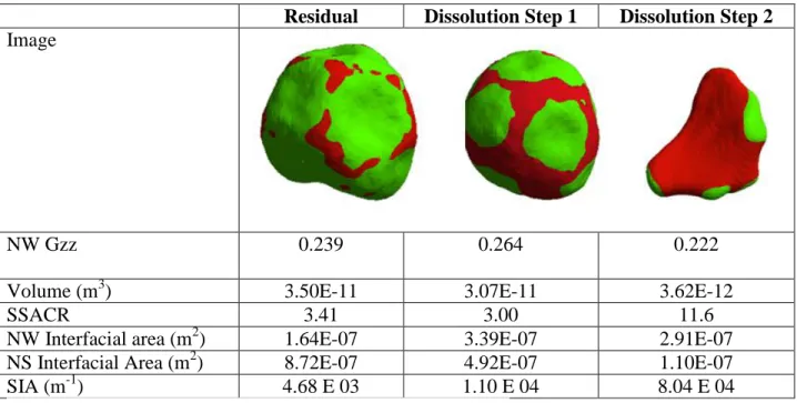
Ian was a medium-sized DNR located in the interior of the column. During the first
dissolution step, the volume of Ian decreased slightly. Additionally, Ian became more rounded,
3 Reeves I, II and III correspond to the top, lower left, and lower right features, respectively.
21
as reflected by SSACR approaching 1.5 (Table 5). The volume of Ian decreased by an order of
magnitude in the second dissolution step. Also during that step, there was a dramatic increase in
NW interfacial area, and consequently SIA. The dissolution pattern of Ian is representative of
many of the DNRs observed. Early in dissolution, many DNRs appear to become more spherical
and experienced only minor changes to volume. Then, the DNRs would experience a sharp
decrease in volume and their geometry changed significantly; changes appear to be dependent on
NAPL contact with mobile wetting fluid.
Table 5. Morphological characteristics of Ian throughout dissolution.
Residual Dissolution Step 1 Dissolution Step 2
Image
NW Gzz 0.239 0.264 0.222
Volume (m3) 3.50E-11 3.07E-11 3.62E-12
SSACR 3.41 3.00 11.6
NW Interfacial area (m2) 1.64E-07 3.39E-07 2.91E-07
NS Interfacial Area (m2) 8.72E-07 4.92E-07 1.10E-07
SIA (m-1) 4.68 E 03 1.10 E 04 8.04 E 04
Comparison of lasting and dissolving DNRs
By constructing a comparison of DNRs that last and DNRs that dissolve, important
characteristics of dissolution may be observed. For each dissolution step, the DNRs that were
fully dissolved were identified. The characteristics of a dissolved DNR were determined for the
22
of the “dissolved” group. If a DNR persisted into a subsequent dissolution step, the
characteristics of that DNR from the preceding dissolution step were used in calculating the
features of the “remain” group. This classification process is presented pictorially in Figure 6.
Figure 6. Conceptual diagram for the classification of DNRs into dissolve and remain groups. Each box represents the volume, curvature, and surface area associated with an individual DNR in a given dissolution step.
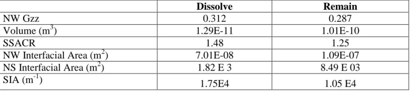
The average orientation, volume, SIA, surface areas and parameterized surface areas for
the dissolved and the remaining DNRs are summarized in Table 6. First, DNRs that dissolved
tended to have their NW interface less oriented in the direction of flow than their counterparts
that remained. On average, dissolved DNRs were an order of magnitude smaller than DNRs that
remained. The SSACR was closer to 1.5 for the dissolve group, indicating that blobs that are
23
is indicative of the fact that dissolved DNRs had a greater contact with the wetting phase relative
to their volume.
Table 6. Orientation, volume, SSACR, surface areas and SIA for DNRs in the remain and dissolve groups.
Dissolve Remain
NW Gzz 0.312 0.287
Volume (m3) 1.29E-11 1.01E-10
SSACR 1.48 1.25
NW Interfacial Area (m2) 7.01E-08 1.09E-07
NS Interfacial Area (m2) 1.82 E 3 8.49 E 03
SIA (m-1) 1.75E4 1.05 E4
DISCUSSION AND CONCLUSION
The current study furthers the scientific understanding of NAPL morphology during
dissolution. Orientation of the NW interface in the direction of flow was observed to be an
important determinant of dissolution. DNRs that dissolved tended to have NW interfaces that
aligned perpendicular to the direction of flow. A NW interface that is aligned with the vertical
direction is likely to have less efficient contact with aqueous phase.
DNRs tended to become less spherical throughout dissolution. This can be attributed to
the fact that many of the smaller blobs, with SSACRs that were close to 1.5 tended to dissolve
early. This finding is echoed by the differences between the dissolve and remain groups. More
spherical DNR, overall, were more likely to dissolve.
Another important parameter assessed in the current study was volume. A decrease in
NAPL volume was anticipated because mass is transferred to the aqueous phase. In the aggregate
system, average volume increased between the residual and the first dissolution step. At first
glance, this finding may seem surprising, given that one would not expect an increase in NAPL
24
dissolution of smaller features between residual and the first dissolution step, creating an average
volume that is greater in the first dissolution step. DNRs that dissolved tended to have smaller
volume than DNRs that remained.
The characterization of the NW interface may prove especially useful, as it may improve
our ability to model the mass transfer of NAPL fluid to the aqueous phase. An increase in SIA
was predicted due to the confluence of two changing parameters. First, the NAPL volume
decreased throughout dissolution. Second, the NW interfacial area increased throughout
dissolution. Generally, the wetting fluid infiltrates a pore body through a pore throat, increasing
the NW interfacial area. However, decreases in SIA may also be observed, particularly if a DNR
is distributed in multiple pore spaces connected by a narrow pore throat. If one of the lobes of
the DNR was to dissolve completely, the overall NW interfacial area could decrease. Of these
two possible phenomena, the former was more common in the DNRs observed, as indicated by
the increase in NW interfacial area exhibited by most DNRs. As observed in all three analyses,
SIA increased throughout dissolution.
The current study was subject to a few important limitations. Most importantly, memory
restrictions for the image processing software, DataTank, would not allow for the processing of
larger NAPL features. This restricted the current study to a subset of smaller DNRs within the
column. Large features contained major portions of the total NAPL volume, so their exclusion
from this study diminishes the utility of findings presented. However, qualitative observation of
the larger DNRs indicates that their dissolution behavior is similar to that of the DNR Reeves.
The large features excluded from study tended to be dissolved into smaller, disconnected
features. If the memory capabilities of DataTank were improved, future studies could analyze
25
Another limitation of the current study is that NAPL morphology was only studied during
three points in dissolution. The kinetics of NAPL dissolution is an important area for study, but
it was difficult to assess the how an individual DNR changed throughout dissolution due to the
limited available images. X-ray micro-tomography is both an expensive and time-consuming
endeavor, so it may not currently be feasible to produce significantly more images. However, if
3-D imaging technologies continue to progress, the cost of imaging could be reduced. A future
study could take images more frequently throughout dissolution to detect smaller changes to a
26 REFERENCES:
Corapcioglu MY, Yoon S, Chowdhurry S. 2002. Pore-scale analysis of NAPL blob dissolution and mobilization in porous media. Transp Porous Med. 79: 419-442.
Flannery BP, Deckman HW, Roberge WG, Damico KL. 1987. 3-Dimensional X-ray microtomography. Science. 237(4821): 1439-1444.
Johns ML, Gladden LF. 1999. Magnetic resonance imaging study of the dissolution kinetics of octanol in porous media. Journal of Colloid and Interface Science 210: 261-270.
Johns ML, Gladden LF. 2001. Surface-to-volume ratio of ganglia trapped in small-pore systems determined by pulsed-filed gradient nuclear magnetic resonance. Journal of Colloid and
Interface Science 238:96-104.
Kachikian C, Harmon TC. 2000. Nonaqueous phase liquid dissolution in porous media: current state of knowledge and research needs. Transport in Porous Media 38:3-28
Miller CT, Poirier-McNeil MM, Mayer AS. 1990. Dissolution of trapped nonaqueous phase liquids: mass transfer characteristics. Water Resources Research 26(11): 2783-2796.
Powers SE, Abriola LM, Dunkin JS, Weber WJ. 1994. Phenomenological models for transient NAPL-water mass-transfer properties. Journal of Contaminant Hydrology 16(1): 1-33.
Schnaar G, Brusseau ML. 2006. Characterizing pore-scale dissolution of organic immiscible liquid in natural porous media using synchotron X-ray microtomography. Environ Sci Technol. 40(21): 6622-6629.