2018_Fang.pdf

A Framework for the Statistical Shape Analysis using SPHARM-PDM

combined with ITK Conformal Flattening Filter

By

Zhengyang Fang

Senior Honors Thesis

Department of Computer Science

University of North Carolina at Chapel Hill

04/27/2018

Approved:

ABSTRACT

Shape analysis is an important and powerful method used in neuroimaging research community

due to its potential to precisely locate morphological changes between healthy and pathological

structures. A popular shape analysis in the neuroimaging community is based on encoding surface

locations in terms of spherical harmonics for a representation called SPHARM–PDM [1] .The

SPHARM-PDM pipeline takes a set of brain segmentation of a single brain structure (for example,

the hippocampus or the caudate nucleus) as input and converts them into a corresponding spherical

harmonic description (SPHARM), which is then sampled into a triangulated surface

(SPHARM-PDM).

At present, the SPHARM-PDM pipeline utilizes heat-equation mapping initialization

parametrization of the surface mesh to the unit sphere and optimization for uniformity of area ratio

between the surface mesh and the parametrized unit sphere. In the case of objects with complex

shape, this initial mapping will suffer from a high degree of mapping distortion that cannot always

be corrected by the following optimization procedure. Here we propose the use of an alternative

initialization parametrization based on the ITK Conformal Flattening filter, which is an

implementation of a paper by Sigurd Angenent, et al., “On the Laplace-Beltrami Operator and

Brain Surface Flatenning” [2] done by Yi Gao, et al. [3]. This method adopts a bijective angle

preserving conformal flattening scheme to replace the heat equation mapping scheme as

initialization parametrization for use in the SPHARM-PDM pipeline. The major scientific

resulting SPHARM surfaces calculated from various structures such as the femur and the mandible

between the original and the newly proposed pipeline, I conclude that in most cases, the new

pipeline produces dramatically better results than the old pipeline based on quantitative measures

of shape. Yet, for some other cases, the conformal flattening based scheme produced marginally

worse results than the heat equation based scheme. The main system contribution of this work is a

command line tool that merges the ITK Conformal Flattening filter into the SPHARM-PDM

pipeline for use in the SALT shape analysis toolbox.

1. INTRODUCTION

For a long time, researchers in the neuro-image area has been using volumetric analysis to assess

the morphology of different brain structures. Even though volume change can be an intuitive

feature to detect dilation and atrophy due to illness, it can be of inadequate help in assessing illness

that cause little to no volume change. To address this issue, neuroimaging community has started

setting its eyes on shape analysis methodology to catch morphological changes between healthy

and pathological structures [1].

In 2006 a framework for the statistical shape analysis of brain structures called SPHARM-PDM

was proposed. Its objective is to bring populations of an anatomic object into optimal

correspondence and thus to allow statistical shape analysis. As we can see from the

SPHARM-PDM shape analysis scheme in figure 1, we start with a segmentation of the brain structures. Next,

using the output binary 3D image, we ensure its spherical topology via the command line tool

following the ‘cracks’ between the foreground (label) and the background. the derived surface

mesh is then mapped to sphere using a method proposed by Brechbühler, et al., “Parametrization

of closed surfaces for 3-D shape description” [4]. The proposed method parametrizes the surface

by defining a continuous, one-to-one mapping from the surface of the original object to the surface

of a unit sphere. It formulates the parametrization as a constraint optimization problem and gets

the practicable starting values by an initial mapping based on a heat equation model. Brechbühler

performs the initialization parametrization considering two criteria:

1. Area preservation: Every object region must map to a region of proportional area in

parameter space, with the constant of proportionality uniform across the surface

2. Minimal distortion: Every quadrilateral of the object should map to a spherical

quadrilateral that has side length equals to the corresponding center angle (in radian) as the

sphere has unit radius in parameter space

Brechbühler then calculates out system of nonlinear equations after establishing constraints for

area preservation with half of the sum of the perimeters of all quadrilaterals being the objective

function. Finally, Brechbühler solves the system of nonlinear equations by linearizing them and

taking Newton steps.

In the fourth step, the framework computes the SPHARM-PDM representation and resolves

correspondence and alignment issues. It takes the surface mesh and its spherical correspondence

as input and produces a series of SPHARM coefficients and SPHARM-PDM meshes, one set in

the original coordinate system, one in the first order ellipsoid aligned coordinate system and one

in the Procrustes aligned coordinate system.However, for complex or skinny objects, the current

degree of distortion that cannot always be corrected by the following optimization procedure.

The final step of the SPHARM-PDM shape analysis framework serves mainly to assess the group

differences of the local surface point distributions by using the StatNonParamTestPDM command

line tool. It can derive two main types of results. a) descriptive group statistics which includes

mean and covariance information; b) group mean difference hypothesis testing.

In 2006, a conformal flattening ITK filter [3] was developed based on the paper by Sigurd

Angenent, et al., “On the Laplace-Beltrami Operator and Brain Surface Flattening” [2]. The

proposed filter performs an angle preserving map of any genus zero (i.e., no handles) surface to

the sphere or to the plane.

In this paper, I propose the use of the above mentioned conformal flattening ITK filter to serve as

the initial parametrization method in the SPHARM-PDM framework by replacing the current heat

equation model based initialization. Specifically, it modified the command line tool called

GenParaMesh used in the third step of the SPHARM-PDM shape analysis framework to improve

the quality of the reconstructed 3D surface mesh (See Figure 2). To test the advantage of the

proposed framework, I employed three datasets of the femur structure, four datasets of the

mandible structure, eight datasets of the mandible condyle structure, sixteen of the molar structure

and four of the cerebral ventricle structure to test both the old and the new SPHARM-PDM pipeline.

Among them, I used two of the three datasets of the femur structure, one of the four datasets of the

mandible structure, one of the eight datasets of the Condyle structure, three of the sixteen datasets

of the molar structure to perform the evaluation between the surface mesh and the SPHARM

mapping initialization parametrization.

I analyzed the datasets results by measuring the mean absolute distance (MAD), average cell area,

the standard deviation of the cell area and by calculating the coefficient of variation of the cell area

between the surface mesh of segmentation and the SPHARM surface mesh in the original

coordinate using two software called MeshValMet [5] and MeshQuality (a tool to analyze cell area

and cell edge ratio developed in UNC Neuro Image Research and Analysis Laboratories(NIRAL)).

As it turns out, the SPHARM surface meshes derived with conformal mapping initialization

parametrization is significantly better in quality than that derived with heat equation mapping

initialization parametrization on complex structures such as the femur and the mandible. The

quality of SPHARM surface meshes with conformal mapping initialization parametrization

converges faster on all datasets than those with heat equation mapping initialization

parametrization notwithstanding with enough iterations, the former is slightly worse than the latter

2. METHODS AND MATERIALS

Our framework for SPHARM-PDM combined with conformal ITK filter consists of five steps:

(1) Segmentation of target organ structures

(2) Post-processing of the segmentations

Segmentation: e.g. using InsightSNAP Output: Binary 3D Image

Segmentation of Brain Structures

Post-processing of the Segmentations

Preprocessing: SegPostProcess Output: Binary 3D Image

Generate Surface Mesh and Parameterized Spheres with Heat Equation Mapping Calculate SPHARM-PDM Representations Statistical testing SPHARM-PDM: ParaToSPHARMMesh Output: SPHARM Coefficients + Aligned Surface

Meshes

(Optional) Statistical Testing: StatNonParamPDM Output: Significance Maps (Raw, Corrected) +

Descriptive Statistics (Mean, Covariance)

Heat Equation Mapping Parameterization: GenParaMesh Output: Surface Mesh + Parametrization

(3) Generation of surface mesh and parametrized spheres with conformal mapping based

initialization parametrization

(4) Calculation of SPHARM-PDM representations

(5) Statistical testing

The newly proposed pipeline is visualized in figure 2. The detailed description of each step lies

on the left of the figure. As you can see, each step utilizes a command line interface tool that

takes the output generated from previous steps as input (except in the first step where we acquire

data from outside sources) and generate respective outputs.

In the third step of our newly proposed framework, I made the contribution by replacing the

complicated sub-steps which uses both GenParaMesh and itkConformalMappingFilter command

line tools into one step, where the user can use only the GenParaMesh command line tool with

Segmentation: e.g. using InsightSNAP Output: Binary 3D Image

Segmentation of Target Organ Structures Post-processing of the Segmentations *Preprocessing: SegPostProcess Output: Binary 3D Image

Generate Surface Mesh and Parameterized Spheres with Conformal Mapping Calculate SPHARM-PDM Representations Statistical testing SPHARM-PDM: ParaToSPHARMMesh

Output: SPHARM Coefficients + Aligned Surface Meshes

(Optional) Statistical Testing: StatNonParamPDM Output: Significance Maps (Raw, Corrected) +

Descriptive Statistics (Mean, Covariance) Heat Equation Mapping Parameterization:

GenParaMesh Output: Surface Mesh

Apply Conformal Mapping Filter: itkConformalMappingFilter

Output: Sphere Mesh

*Conformal Mapping Parameterization: GenParaMesh Output: Surface Mesh + Conformal Parametrization

Figure 2: I proposed the modified SPHARM-PDM shape analysis framework utilizing conformal flattening filter as the initial parametrization method

2.1 Subjects and Acquisition

I applied both the newly proposed SPHARM-PDM shape analysis framework with conformal

mapping initialization parametrization and the original SPHARM-PDM shape analysis

framework with heat equation initialization parametrization to five datasets (the femur, the

mandible, the molar, the condyle and the ventricle) acquired from different sources.

From these data, I used the following outputs generated in the pipeline to measure and compare

the quality of the reconstructed SPHARM surface meshes using either the old or the new

SPHARM-PDM framework:

(1) Surface mesh of the segmentation obtained in the GenParaMesh step

(2) SPHARM surface mesh in the original coordination system obtained in the

ParaToSPHARMMesh Step

2.1.1 The Femur Data Reference

The femur data were obtained from a collaboration with the University of Bern in 2004. The

exact origin of the data is unfortunately unknown.

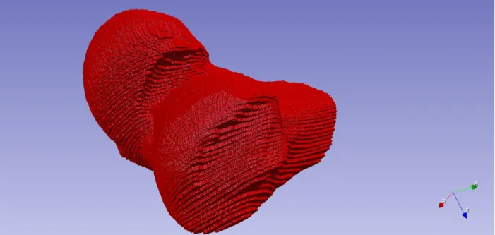
Figure 3: One of the three Femur volumes visualized in 3D Slicer [11] Volume Module

2.1.2 The Mandible & The Condyle Data Reference

The mandible and Condyle data was a subset of the data used in the study “3D superimposition

and understanding temporomandibular joint arthritis” [6]. In the original study, the Department

of Orthodontics and Pediatric Dentistry at the University of Michigan acquired Cone beam CT

scans from 69 subjects with long-term temporomandibular joint (TMJ) osteoarthritis (OA, mean

age 39.1 ± 15.7 years), 15 subjects at initial consult diagnosis of OA (mean age 44.9 ± 14.8

years), and seven healthy controls (mean age 43 ± 12.4 years).

The original data format of the condyle data was vtk, but the GenParaMesh command line tool

does not accept vtk file format as input file format. Therefore, UNC graduate student Mahmoud

Mostapha used an open source command line tool called PolyDataToImageData to convert the

original vtk poly data files into nrrd file format [12].

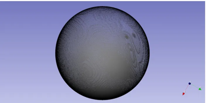
Figure 4: One of the four Mandible volumes visualized in 3D Slicer [11] Volume Module

2.1.3 The Molar Data Reference

The molar data used in my study is a subset of the data used in the study of [7] and “Group-wise

shape correspondence of variable and complex objects” [8], and a detailed explanation of sample

preparation can be found in [9]. In short, molds of actual tooth-rows were molded using a

polyvinylsiloxane material (PresidentJet Plus) and cast in epoxy EpoTek 301. The second

mandibular molar was trimmed from the tooth row and scanned with the Scanco µCT-40

machine at Stony Brook University's Center for Biotechnology. Three-dimensional surfaces of

each tooth were segmented from the resulting DICOM or TIFF stacks using Amira 5.1 or Avizo

6.0.

2.1.4 The Ventricle Data Reference

High-resolution MRI scans were acquired from three different subject groups [10 monozygotic

(MZ) twin pairs discordant for schizophrenia (DS), 9 healthy MZ twin pairs, and 10 healthy

gender, and handedness. A fourth group consisting of 10 healthy nonrelated (NR) subject pairs

also matched for age, gender, and handedness was selected from the two healthy groups.

Volumetric differences as well as 3D maps representing magnitude and significance of shape

differences between the twin pairs and between subject groups were computed and visualized.

These dataset was then processed by using a rater-independent, automatic tissue-segmentation

method. For detail of the image processing, see the Image Processing section in “Morphometric

analysis of lateral ventricles in schizophrenia and healthy controls regarding genetic and

disease-specific factors” [10].

2.2 Original Surface Mesh

I first use the SegPostProcess command line tool to extract a single binary label and apply

heuristic methods to ensure the spherical topology of the segmentation. After this, I apply

GenParaMesh command line tool to compute the surface mesh corresponding to the

segmentation. I obtain the surface meshes of the segmentations and compare them with the

SPHARM surface with either heat equation mapping initialization parametrization or conformal

mapping initialization parametrization.

2.3 SPHARM Surface Mesh

I apply the GenParaMesh command line tool with different iterations and with either heat

equation mapping initialization parametrization or conformal mapping initialization

parametrization. Specifically, using the original heat equation mapping initialization

parametrization, I pick 0, 50, 100, 150 … 500 iterations and save the surface meshes and their

parametrized spheres. With conformal mapping initialization parametrization, I pick the same

number of iterations as with heat equation mapping initialization parametrization. Before I

develop the command line tool to perform GenParaMesh with conformal mapping initialization

parametrization, in order to test the newly proposed pipeline, I first apply GenParaMesh with 0

iterations (to save computing time) to get the surface mesh, then use the conformal mapping

command line tool to convert the surface mesh to conformal mapping based parametrized sphere,

next set the conformal mapping parametrized sphere as the initialization parametrization through

the “--initPara” option of the GenParaMesh command line tool and lastly set the number of

iteration to be 0, 50, 100,150 … 500 for comparison with the original pipeline. I then apply the

ParaToSPHARMMesh command line tool using the surface mesh and the parametrized sphere

with different iterations and with either heat equation mapping initialization parametrization or

conformal mapping initialization parametrization as inputs and obtain the output SPHARM

surface mesh in the original coordinate system for comparison with the surface mesh of the

segmentation.

It is important to let researchers in neuro-imaging community use SPHARM-PDM with

conformal mapping initialization parametrization conveniently. Thus, I developed a command

line tool based on the Slicer Execution Model that will be used in the Slicer SALT Shape

Analysis Toolbox in the future. Before the command line tool was developed, researchers has to

do the following in order to apply GenParaMesh command line tool with conformal mapping

initialization parametrization:

(1) Apply GenParaMesh command line tool on the target dataset with 0 iteration (to save

computing time) to obtain the surface mesh of the segmentation

(2) Apply the ITK conformal flattening filter command line tool on the surface mesh to obtain

the conformal parametrized sphere

(3) Apply the GenParaMesh command line tool with the conformal parametrized sphere as the

initialization parametrization by setting the “--initPara” option in the GenParaMesh command

line tool

With the new tool, researchers only need to set the “—conf” flag on in the GenParaMesh

command line tool in order to use conformal mapping initialization parametrization.

During each usage of GenParaMesh with “--conf” flag, three intermediate files will be written to

the output directory. Specifically they are

(1) $ppcase-iter[iteration number]-surf0.vtk

(3) $ppcase-iter[iteration number]-confPara0.meta

The first file is the surface mesh of segmentation. The second file is the parametrized sphere of

the surface mesh with conformal mapping initialization parametrization. The third file is the

“meta” format version of the second file which has to be created due to code implementation

reason. To enable the user to apply the GenParaMesh command line tool with conformal

mapping initialization parametrization in parallel to the datasets, I assign each intermediate file a

unique name associated with its label name ($ppcase) and iteration number.

3. RESULTS

To test the proposed framework, I used the condyle, the femur, the mandible, the molar and the

ventricle datasets as discussed in Subjects and Acquisition section. The surface mesh of the

segmentation and the SPHARM surface mesh were computed with either heat equation mapping

initialization parametrization or conformal mapping initialization parametrization. There are two

kinds of statistics that can help us to evaluate the quality of the reconstructed SPHARM surface:

(1) Measurement of the distance from the original surface mesh to the reconstructed SPHARM

surface mesh between two triangle meshes using uniform sampling

(2) Measurement of the average cell (it is not to be confused with the word “cell” used in the

field of biology; in this context, the word “cell” means a triangle of the surface mesh) area of the

SPHARM surface, standard deviation of cell area of the SPHARM surface and the coefficient of

variation of cell area of the SPHARM surface by dividing the standard deviation of cell area of

It is clear that the quality of the reconstructed SPHARM surface can be determined by its

distance to the original surface; therefore, the first measurement is a perfectly valid measurement

of the goodness of the reconstructed SPHARM surface. Because of the uniform cell

correspondence across the SPHARM surface between the parametrized sphere and the SPHARM

surface, the coefficient of variation of the cell area of the SPHARM surface is equal to the

coefficient of variation of the cell area of the parametrized sphere. Since the variation of cell area

of the parametrized sphere is a determining factor of the quality of the approximation of the

original surface mesh, the coefficient of variation of the cell area of the SPHARM surface mesh

is also a valid measure of the quality of SPHARM reconstruction, i.e., the second measurement

is also valid. It is clear that the first measurement is the best when its value becomes zero, when

the original surface mesh and the reconstructed SPHARM surface mesh are completely

overlapping, i.e., identical. Because the optimization procedure of the GenParaMesh step

converges when the triangles of the parametrized sphere have equal area, the standard deviation

of the cell area of the SPHARM surface approaches zero when the quality of the surface is the

best. Therefore, the second measurement also becomes better as its value gets closer to zero.

Therefore, to measure the quality of these SPHARM surface meshes, my advisor, Dr. Martin

Styner, and I carefully chose two software tools for statistical shape analysis: MeshValMet [5]

and MeshQuality (a command line tool developed by UNC PhD student Mahmoud Mostapha at

the Neuro Image Research and Analysis Laboratories (NIRAL) of the University of North

Carolina at Chapel Hill) with each one of them produces one of the two kinds of shape statistics

Distance (MAD) between the original surface mesh and the reconstructed SPHARM surface

mesh by averaging the sum of absolute distance between each vertex of the original surface and

the SPHARM surface. When utilizing the MeshValMet software, I import the original surface

mesh as model A (abbreviated A) and the reconstructed SPHARM surface mesh as model B

(abbreviated B), then I set the “sampling step” to be “0.5%”, the “minimum sampling frequency”

to be “2”, compute settings to be “A->B, B->A”, “number of bins” to be “256” and let

“compute” be “signed distance”. With 0.5% sampling step and 2 minimum sampling frequency,

MeshValMet can compute the distance between model A and model B in the error space with a

fine sampling level; due to assymetric property of the Hausdorff distance, I choose “A->B,

B->A” as the compute setting; since we do not need the histogram information in the

MeshValMet software, I leave the “number of bins” to be its default value – “256”; since I only

need the absolute distance between model A and model B, I choose “absolute distance” in the

“compute” option. With the reconstructed SPHARM surface as input, MeshQuality command

line tool can produce Average Cell Area of the SPHARM surface, Standard Deviation of Cell

Area of the SPHARM surface and the Coefficient of Variance of Cell Area of the SPHARM

surface by dividing the Standard Deviation of Cell Area of the SPHARM surface by the Average

Cell Area of the SPHARM surface. Ideally, we only need the MAD to measure the quality of

SPHARM surface mesh, but since MeshValMet tool will crash while analyzing some of the

datasets, we have to adopt the MeshQuality command line tool to calculate the Coefficient of

Variance of Cell Area of the SPHARM surface to measure the quality of SPHARM surface

mesh. I collected all the data and used line charts to quantitatively show the quality of the

SPHARM surface meshes with either one of the two different initialization parametrizations. As

suggests better reconstruction quality as its value approaches 0. The coefficient of variation of

cell area is an intermediate measure of goodness that also indicates better reconstruction quality

as its value approaches 0.

The femur datasets:

All three of the femur volume datasets can be successfully reconstructed with both heat equation

mapping initialization parametrization and conformal mapping initialization parametrization. I

measured two of the three datasets of the femur using MeshValMet [5] and MeshQuality and

record and visualize the result in line charts to show the quality of SPHARM surface meshes with

either heat equation mapping initialization parametrization or conformal mapping initialization

parametrization.

(1) The femur dataset labeled 001:

Figure 9: Heat equation mapping as initialization parametrization parametrized sphere of the femur dataset labeled 001 with iteration 0. It has bad quality because of the great variation in size of all triangles across the surface. Visualized in 3D Slicer [11]

Model Module.

Figure 10: Conformal mapping as initialization parametrization parametrized sphere of the femur dataset labeled 001 with iteration 0. Even though it has very densely populated area (the dark regions), It is still a great initialization

Figure 11: Heat equation mapping as initialization parametrization parametrized sphere of the femur dataset labeled 001 with iteration 50, which still have a bad quality given the large variation in the size of triangles across the sphere. It is similar in

quality compared to the heat equation mapping as initialization parametrization parametrized sphere with iteration 0. Visualized in 3D Slicer [11] Model Module.

Figure 12: Conformal mapping as initialization parametrization parametrized sphere of the femur dataset labeled 001 with iteration 50. The quality has been improved as the triangles become more uniformly distributed and there are no more densely

Figure 13: Heat equation mapping as initialization parametrization parametrized sphere of the femur dataset labeled 001 with iteration 100. It still has poor quality overall. Visualized in 3D Slicer [11] Model Module.

Figure 14: Conformal mapping as initialization parametrization parametrized sphere of the femur dataset labeled 001 with iteration 100. It has better quality than the conformal mapping as initialization parametrization parametrized sphere with

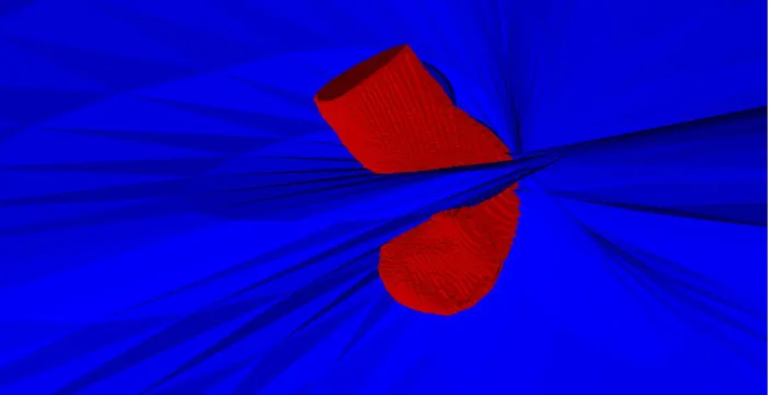
Figure 15: The overlay of the original surface mesh (red) of the femur dataset labeled 001 and the SPHARM surface mesh of it with heat equation mapping initialization parametrization with iteration 500 (blue). Since the SPHARM surface (blue) does not even look like the femur structure, it is clear that the SPHARM surface with heat equation mapping initialization parametrization

failed to provide a good representation of the original surface mesh. Visualized in 3D Slicer [11] Model Module.

Figure 16: The overlay of the original surface mesh (red) of the femur dataset labeled 001 and the SPHARM surface mesh of it with conformal mapping initialization parametrization with iteration 500 (blue). Since the SPHARM surface with conformal mapping initialization parametrization looks like the femur structure and has a lot of overlapping regions, the SPHARM surface

Figure 17: The femur dataset labeled 001 Mean Absolute Distance (MAD). MeshValMet Software failed to make measurement after 50 iterations between the SPHARM surface mesh with heat equation mapping initialization parametrization and the original surface, so the orange line has blanks after 50 iterations. With this much information, it is still clear that conformal mapping initialization parametrization performs very well and consistent in quality on the femur data, yet the SPHARM surface

with heat equation mapping initialization parametrization has poor quality overall.

Figure 18: the femur dataset labeled 001 Coefficient of Variation of Cell Area. MeshQuality command line tool crashed when measure the SPHARM surface mesh with heat equation mapping initialization parametrization, so there is a blank on the orange

line. However, it is obvious that the SPHARM surfaces with heat equation mapping initialization parametrization has poor and consistent quality overall. And it agrees with the result as suggested in the MAD chart that conformal mapping initialization

parametrization provides SPHARM surface meshes with good and consistent quality

0.54 0.51 0.49 0.47 0.45 0.43 0.41 0.40 0.39 0.39 0.39

4.04 48.23 0.00 10.00 20.00 30.00 40.00 50.00 60.00

0 50 100 150 200 250 300 350 400 450 500

The Femur Dataset Labeled 001 MAD

Conformal Mapping Heat Equation Mapping

Milimeters

Iterations

96% 91% _{82% 72%}

67% 62% 58% 54% 51% 47% 44%

359%

492%

464% _449%

434% _{424% 428%}

411% 440% 436%

0% 100% 200% 300% 400% 500% 600%

0 50 100 150 200 250 300 350 400 450 500

The Femur Dataset Labeled 001 Coefficient of Variation of Cell Area

Conformal Mapping Heat Equation Mapping

The blank spaces were caused by failure of the software to analyze data. Still, with the information

acquired, we can see that the quality of SPHARM surface with conformal mapping initialization

parametrization is significantly better than that with heat equation mapping initialization

parametrization.

(2) The femur dataset labeled 002:

Figure 20: Heat equation mapping as initialization parametrization parametrized sphere of the femur dataset labeled 002 with iteration 0. Because the variation of the triangle size is huge, it has a poor quality. Visualized in 3D Slicer [11] Model Module.

Figure 21: Conformal mapping as initialization parametrization parametrized sphere of the femur dataset labeled 002 with iteration 0. It is a parametrized sphere with small variation in size of triangles and has near uniform density. It can be improved

Figure 22: Heat equation mapping as initialization parametrization parametrized sphere of the femur dataset labeled 002 with iteration 50. Since the size of large triangles becomes larger than those in 0 iteration, the quality also becomes poorer. Visualized in 3D Slicer [11] Model Module.

Figure 24: Heat equation mapping as initialization parametrization parametrized sphere of the femur dataset labeled 002 with iteration 100. Since the uniformity of triangle size has increased, it has improved in quality from the one with iteration 50 (even though still not great). Visualized in 3D Slicer [11] Model Module.

Figure 26: The overlay of the original surface mesh (red) of the femur dataset labeled 002 and the SPHARM surface mesh of it with heat equation mapping initialization parametrization with iteration 500 (blue). Since the SPHARM surface (blue) does not even look like the femur structure, it is clear that the SPHARM surface with heat equation mapping initialization parametrization failed to provide a good representation of the original surface mesh. Visualized in 3D Slicer [11] Model Module.

Figure 27: The overlay of the original surface mesh (red) of the femur dataset labeled 002 and the SPHARM surface mesh of it with conformal mapping initialization parametrization with iteration 500 (blue). Since the SPHARM surface with conformal mapping initialization parametrization looks like the femur structure and has a lot of overlapping regions, the SPHARM surface

Figure 28: The femur dataset labeled 002 Mean Absolute Distance (MAD). MeshValMet Software failed to make measurement

between the SPHARM surface mesh with heat equation mapping initialization parametrization and the original surface, so

unfortunately, I am unable to compare the mean absolute distance in this dataset. However, it is certain that the conformal

mapping initialization parametrization performs well.

Figure 29: The femur dataset labeled 002 Coefficient of Variation of Cell Area. It is clear that conformal mapping initialization

parametrization is better than heat equation mapping initialization parametrization for the femur dataset labeled 002. In

general, the heat equation mapping initialization parametrization does 4-5 times worse than the conformal mapping

initialization parametrization and nearly 10 times worse when iteration increases to 500

0.54 0.51 0.48 0.46 0.44 0.51 0.41 0.40 0.39 0.39 0.38

0 1 2 3 4 5 6 7 8 9 10

0 100 200 300 400 500 600

The Femur Dataset Labeled 002 MAD with Conformal ITK filter Milimeters

Iterations

96% 91% 81% 72% 67% 62% 58% 54% 50% 47% 44%

357%

489% _465%

447% 434% 425% 420% _393% 431% 428% 434%

0% 100% 200% 300% 400% 500% 600%

0 50 100 150 200 250 300 350 400 450 500

The Femur Dataset Labeled 002 Coefficient of Variation of Cell Area

Conformal Mapping Heat Equation Mapping

Since we are only able to acquire the MAD of SPHARM surface mesh with conformal mapping

initialization parametrization because of the MeshValMat software’s limitation, we can only argue

that conformal mapping initialization parametrization performs well on the femur dataset labeled

002. With the Coefficient of Variation of Cell Area chart, we can clearly see that the quality of the

SPHARM surface meshes with conformal mapping initialization parametrization is significantly

better than those with heat equation mapping initialization parametrization for the femur datasets.

The molar datasets:

All of the sixteen Molar datasets can be reconstructed as SPHARM surface using either conformal

mapping initialization parametrization or heat equation mapping initialization parametrization. I

measured three of the sixteen datasets to compare the quality of reconstructed SPHARM surface

with two initialization parametrization.

Figure 30: Surface mesh of the molar Dataset labeled a10, which is the output of GenParaMesh and will then be mapped onto

parametrized spheres with different iterations. Visualized in 3D Slicer[11] Model Module.

Figure 11: Heat equation mapping as initialization parametrization parametrized sphere of the molar dataset labeled a10 with iteration 0, it is not a good parametrization because it has a large variation in triangle size. Visualized in 3D Slicer [11] Model

Figure 32: Conformal mapping as initialization parametrization parametrized sphere of the molar dataset labeled a10 with iteration 0. It is a parametrized sphere with small variation in size of triangles and has near uniform density. Visualized in 3D

Slicer [11] Model Module.

Figure 33: Heat equation mapping as initialization parametrization parametrized sphere of the molar dataset labeled a10 with iteration 50, it is still not a good parametrization because it has a large variation in the size of triangles (even though increasing

Figure 34: Conformal mapping as initialization parametrization parametrized sphere of the molar dataset labeled a10 with iteration 50. It is a parametrized sphere with small variation in size of triangles and has near uniform density. However, it does

not improve much from iteration 0. Visualized in 3D Slicer [11] Model Module.

Figure 35: Heat equation mapping as initialization parametrization parametrized sphere of the molar dataset labeled a10 with iteration 100, it is an extremely good parametrization since it has excellent uniformity in triangle size and even looks slightly better compared with conformal mapping initialization parametrization parametrized sphere with same number of iterations.

Figure 36: Conformal mapping as initialization parametrization parametrized sphere of the molar dataset labeled a10 with iteration 100. It is a parametrized sphere with small variation in size of triangles and has near uniform density and is consistent

in quality as the one with iteration 0 and 50. Visualized in 3D Slicer [11] Model Module.

Figure 37: The overlay of the original surface mesh (red) of the molar dataset labeled a10 and the SPHARM surface mesh of it with heat equation mapping initialization parametrization with iteration 500 (blue). It has extremely high level of overlay since the blue and the red one intervened with each other; both have the correct and similar shape. Visualized in 3D Slicer [11] Model

Figure 38: The surface mesh overlay of the femur dataset labeled 002 of the original surface mesh (red) and the SPHARM surface mesh with conformal mapping initialization with iteration 500 (blue). It is hard to tell whether conformal mapping initialization parametrization or heat equation initialization parametrization is better because both have similar level of overlapping with the

original surface and slimier shape as the original surface. Visualized in 3D Slicer [11] Model Module.

Figure 39: Molar Dataset Labeled a10 Mean Absolute Distance (MAD). Clearly, the heat equation mapping initialization parametrization does poorly with 0 iteration but the improvement by the following optimization procedure is huge. On the

contrary, the conformal mapping initialization parametrization does extremely well with 0 iterations and performs very consistently with more iterations. Surprisingly, the heat equation mapping initialization parametrization, after being corrected

by its following optimization procedure, does slightly better than conformal mapping initialization parametrization 0.0167 0.0147 0.0140 0.0089 0.0089 0.0132 0.0130 0.0128 0.0127 0.0126 0.0124 0.1833

0.0097 0.0089 0.0089 0.0089 0.0089 0.0089 0.0089 0.0089 0.0089 0.0089

0.00 0.02 0.04 0.06 0.08 0.10 0.12 0.14 0.16 0.18 0.20

0 100 200 300 400 500 600

The Molar Dataset Labeled a10 MAD

Conformal Mapping Heat Equation Mapping

Figure 40: Molar Dataset Labeled a10 Coefficient of Variation of Cell Area. At iterations 0, heat equation mapping initialization parametrization performs extremely bad but when iteration number becomes larger, it quickly converges to a level of extremely

good quality. Comparatively, conformal mapping initialization parametrization does well on 0 iteration but the optimization procedure does not improve its quality too much. With iterations at or above 50 (at most), the heat equation mapping

initialization parametrization outperforms the conformal mapping initialization parametrization.

The molar dataset labeled a13:

Figure 41: Surface mesh of the molar Dataset labeled a13, which is the output of GenParaMesh and will then be mapped onto

parametrized spheres with different iterations. Visualized in 3D Slicer [11] Model Module. 74%

70% _66%

63% _61%

59% _57%

55% _{53% 52%}

50%

32%

16% 15% 15% 15% 15% 15% 15% 15% 15%

0% 20% 40% 60% 80% 100% 120%

0 100 200 300 400 500 600

The Molar Dataset Labeled a10 Coefficient of Variation of Cell Area

Conformal Mapping Heat Equation Mapping

2044%

Figure 42: Heat equation mapping as initialization parametrization parametrized sphere of the molar dataset labeled a13 with iteration 0, it is not a good parametrization because the variation of triangle size is huge. Visualized in 3D Slicer [11] Model

Module

Figure 43: Conformal mapping as initialization parametrization parametrized sphere of the molar dataset labeled a13 with iteration 0. It is a parametrized sphere with small variation in size of triangles and has near uniform density. Visualized in 3D

Figure 44: Heat equation mapping as initialization parametrization parametrized sphere of the molar dataset labeled a13 with iteration 50, it is not a good parametrization because it has a large variation in triangle size but it is better (increase in

uniformity of triangle size) than iteration 0. Visualized in 3D Slicer [11] Model Module

Figure 45: Conformal mapping as initialization parametrization parametrized sphere of the molar dataset labeled a13 with iteration 50. It is a parametrized sphere with small variation in size of triangles and has near uniform density, consistent in

Figure 46: Heat equation mapping as initialization parametrization parametrized sphere of the molar dataset labeled a13 with iteration 100, it is not a good parametrization because it has a large variation of triangle size, but it is better (increase in

uniformity of triangle size) than iteration 50. Visualized in 3D Slicer [11] Model Module

Figure 47: Conformal mapping as initialization parametrization parametrized sphere of the molar dataset labeled a13 with iteration 100. It is parametrized sphere with small variation in size of triangles and has near uniform density, consistent with the

Figure 48: The surface mesh overlay of the molar dataset labeled a13 of the original surface mesh (red) and the SPHARM surface mesh with heat equation mapping initialization parametrization with iteration 500 (blue). The rate of overlapping and the level

of similarity between the two surfaces is high, so the reconstruction quality is fairly good. Visualized in 3D Slicer [11] Model Module.

Figure 49: The surface mesh overlay of the molar dataset labeled a13 of the original surface mesh (red) and the SPHARM surface mesh with conformal mapping initialization parametrization with iteration 500 (blue). The quality of reconstruction is also good.

Figure 50: Molar Dataset Labeled a13 Mean Absolute Distance (MAD). The pattern is similar to that of the molar dataset

labeled a10.

Figure 51: Molar Dataset Labeled a13 Coefficient of Variation of Cell Area. The pattern of Coefficient of variation of Cell Area is

similar to that of the molar dataset labeled a10. 0.0165 0.0147 0.0137

0.0087 0.0087 0.0123 0.0119 0.0117 0.0115 0.0114 0.0112 0.1381

0.0137 0.0094

0.0087 0.0086 0.0085 _0.0085 0.0085 0.0085 0.0085 0.0085

0.00 0.02 0.04 0.06 0.08 0.10 0.12 0.14 0.16 0.18 0.20

0 50 100 150 200 250 300 350 400 450 500

The Molar Dataset Labeled a13 MAD

Conformal Mapping Heat Equation Mapping _Iterations

Milimeters

89% 85%

81% _79%

76% _{74% 72%}

70% _{69% 67%}

65% 68%

32%

20% 20% 20% 20% 20% 20% 20% 20%

0% 20% 40% 60% 80% 100% 120%

0 50 100 150 200 250 300 350 400 450 500

The Molar Dataset Labeled a13 Coefficient of Variation of Cell Area

Conformal Mapping Heat Equation Mapping Iterations

The molar dataset labeled b01:

Figure 52: Surface mesh of the molar Dataset labeled b01, which is the output of GenParaMesh and will then be mapped onto parametrized spheres with different iterations. Visualized in 3D Slicer [11] Model Module.

Figure 53: Heat equation mapping as initialization parametrization parametrized sphere of the molar dataset labeled b01 with iteration 0, it is not a good parametrization because it has a large variation in size of triangles. Visualized in 3D Slicer [11] Model

Figure 54: Conformal mapping as initialization parametrization parametrized sphere of the molar dataset labeled b01 with iteration 0. It is parametrized sphere with small variation in size of triangles and has near uniform density. Visualized in 3D Slicer

[11] Model Module.

Figure 55: Heat equation mapping as initialization parametrization parametrized sphere of the molar dataset labeled b01 with iteration 50, it is not a good parametrization because it has a large variation in size of triangles, but it is better (increase in

Figure 56: Conformal mapping as initialization parametrization parametrized sphere of the molar dataset labeled b01 with iteration 50. It is a parametrized sphere with small variation in size of triangles and has near uniform density, consistent with the

one with iteration 0. Visualized in 3D Slicer [11] Model Module.

Figure 57: Heat equation mapping as initialization parametrization parametrized sphere of the molar dataset labeled b01 with iteration 100, it is not a good parametrization because it has a uniform distributed size of triangles, but it is better (increase in

Figure 58: Conformal mapping as initialization parametrization parametrized sphere of the molar dataset labeled b01 with iteration 100. It is a parametrized sphere with small variation in size of triangles and has near uniform density and is consistent

in quality with iteration 0 and 50. Visualized in 3D Slicer [11] Model Module.

Figure 60: The surface mesh overlay of the molar dataset labeled b01 of the original surface mesh (red) and the SPHARM surface mesh with conformal mapping initialization with iteration 500 (blue). It also has a great reconstruction quality. But It is hard to tell whether conformal mapping initialization parametrization or heat equation initialization parametrization is better through

visualization. Visualized in 3D Slicer [11] Model Module.

Figure 61: Molar Dataset Labeled b01 Mean Absolute Distance (MAD). The pattern is similar to that of the molar dataset labeled

a10 and a13. 0.0165 0.0147 _0.0137

0.0087 0.0087 _0.0123 0.0119 0.0117 0.0115 0.0114 0.0112 0.1381

0.0137 0.0094 0.0087 0.0086 0.0085 0.0085 0.0085 0.0085 0.0085 0.0085

0 0.02 0.04 0.06 0.08 0.1 0.12 0.14 0.16 0.18 0.2

0 50 100 150 200 250 300 350 400 450 500

The Molar Dataset Labeled b01 MAD

Figure 62: Molar Dataset Labeled a13 Coefficient of Variation of Cell Area. The pattern of Coefficient of variation of Cell Area is

similar to that of that of the molar dataset labeled a10 and a13.

For molar data, we can clearly see that conformal mapping initialization parametrization performs much better than heat equation mapping initialization parametrization with few iterations and it converges faster than the heat equation mapping initialization parametrization. However, with larger iteration number, conformal mapping initialization parametrization

performs slightly worse than the heat equation mapping initialization parametrization.

The mandible dataset:

From the four Mandible datasets acquired, I successfully reconstructed one of them following the

SPHARM-PDM pipeline with both conformal mapping method and heat equation mapping

method.

116% _113%

111% _108%

107% _{105% 104%}

102% 101% 100% 99%

85%

21% 21% 20% 20% 20% 20% 20% 20% 20%

0% 20% 40% 60% 80% 100% 120%

0 50 100 150 200 250 300 350 400 450 500

The Molar Dataset Labeled b01 Coefficient of Variation of Cell Area

The mandible dataset labeled 002:

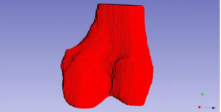
Figure 63: Surface mesh of the mandible dataset labeled 002, which is the output of GenParaMesh and will then be mapped onto parametrized spheres with different iterations. Visualized in 3D Slicer [11] Model Module.

Figure 64: Heat equation mapping as initialization parametrization parametrized sphere of the mandible dataset labeled 002 with iteration 0, it is not a good parametrization because it has a huge variation in triangle size. Visualized in 3D Slicer [11]

Figure 65: Conformal mapping as initialization parametrization parametrized sphere of the mandible dataset labeled 002 with iteration 0. It is a parametrized sphere with small variation in size of triangles and has near uniform density. Visualized in 3D

Slicer [11] Model Module.

Figure 67: Conformal mapping as initialization parametrization parametrized sphere of the mandible dataset labeled 002 with iteration 50. It is a parametrized sphere with small variation in size of triangles and has near uniform density. Visualized in 3D

Slicer [11] Model Module.

Figure 68: Heat equation mapping as initialization parametrization parametrized sphere of the mandible dataset labeled 002 with iteration 100, it is slightly improved in triangle uniformity in triangle uniformity from 50 iterations. Visualized in 3D Slicer

Figure 69: Conformal mapping as initialization parametrization parametrized sphere of the mandible dataset labeled 002 with iteration 100. It is parametrized sphere with small variation in size of triangles and has near uniform density. Visualized in 3D

Slicer [11] Model Module.

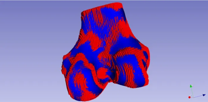
Figure 70: The surface mesh overlay of the mandible dataset labeled 002 of the original surface mesh (red) and the SPHARM surface mesh with heat equation mapping initialization parametrization with iteration 500 (blue). The level of overlapping and

Figure 71: The surface mesh overlay of the mandible dataset labeled 002 of the original surface mesh (red) and the SPHARM surface mesh with conformal mapping initialization with iteration 500 (blue). It also has a good quality. But it is hard to tell whether conformal mapping initialization parametrization or heat equation initialization parametrization is better through

visualization. Visualized in 3D Slicer [11] Model Module.

Figure 72: Mandible dataset Labeled 002 Mean Absolute Distance (MAD). It is clear that the heat equation mapping

initialization parametrization both performs worse and is less stable than conformal mapping initialization parametrization. The

irregularity of the quality of heat equation mapping initialization parametrization suggests the mandible structure is unstable

with the optimization procedure of the GenParaMesh. 2.93

1.60 1.14 0.89 0.73 0.64 0.59 0.55 0.52 _{0.50 0.48}

6.43 41.55 37.49 20.09 29.54 34.87 30.65 32.77

0.52 _4.85 0.62

0 5 10 15 20 25 30 35 40 45

0 50 100 150 200 250 300 350 400 450 500

The Mandible Dataset Labeled 002 MAD

Conformal Mapping Heat Equation Mapping _Iterations

Figure 73: Mandible dataset Labeled 002 Coefficient of Variation of Cell Area. The pattern of Coefficient of variation of Cell Area

is similar to that of Mean Absolute Distance (MAD). Mesh Quality software failed to analyze the data at 400 iterations, so there

is a blank at 400 iterations.

From the mandible dataset, we can see a very clear comparison of MAD and coefficient of

variation value between two initialization parametrization. As it turns out, the conformal mapping

initialization parametrization yields a significantly better result of MAD and coefficient of

variation of cell area than the heat equation mapping initialization parametrization.

The condyle dataset:

All Condyle data can be analyzed through both the old and the newly proposed SPHARM-PDM

pipeline. I picked one of the nine Condyle datasets to investigate the quality of 3D reconstruction

with different initialization parametrization.

206% 201% 196% 187% 178% 170% 161% 154% 146% 140% 134%

290%

531% 525%

445% 509%

542% 534% _507%

414% 96% 0 1 2 3 4 5 6

0 50 100 150 200 250 300 350 400 450 500

The Mandible Dataset Labeled 002 Coefficient of Variation of Cell Area

Conformal Mapping Heat Equation Mapping

The condyle dataset labeled AC10_Left:

Figure 74: Surface mesh of the condyle Dataset labeled AC10_Left, which is the output of GenParaMesh and will then be

mapped onto parametrized spheres with different iterations. Visualized in 3D Slicer [11] Model Module.

Figure 75: Heat equation mapping as initialization parametrization parametrized sphere of the condyle Dataset labeled AC10_Left with iteration 0, it is not a good parametrization because it has an extremely large variation in triangle size.

Figure 76: Conformal mapping as initialization parametrization parametrized sphere of the condyle Dataset labeled AC10_Left with iteration 0. It is a parametrized sphere with small variation in size of triangles and has near uniform density. Visualized in

3D Slicer [11] Model Module.

Figure 77: Heat equation mapping as initialization parametrization parametrized sphere of the condyle Dataset labeled AC10_Left with iteration 50, it is a parametrized sphere with small variation in size of triangles and has a near uniform density

Figure 78: Conformal mapping as initialization parametrization parametrized sphere of the condyle Dataset labeled AC10_Left with iteration 50. It is a parametrized sphere with small variation in size of triangles and has near uniform density. Visualized in

3D Slicer [11] Model Module.

Figure 79: Heat equation mapping as initialization parametrization parametrized sphere of the condyle Dataset labeled AC10_Left with iteration 100, it is parametrized sphere with small variation in size of triangles and has near uniform density.

Figure 78: Conformal mapping as initialization parametrization parametrized sphere of the condyle Dataset labeled AC10_Left with iteration 100. It is a parametrized sphere with small variation in size of triangles and has near uniform density. Visualized in

3D Slicer [11] Model Module.

Figure 79: The surface mesh overlay of the condyle Dataset labeled AC10_Left of the original surface mesh (red) and the SPHARM surface mesh with heat equation mapping initialization with iteration 500 (blue). The level of similarity and the rate of

Figure 80: The surface mesh overlay of the condyle Dataset labeled AC10_Left of the original surface mesh (red) and the SPHARM surface mesh with conformal mapping initialization with iteration 500 (blue). It also has a great reconstruction quality.

But it is hard to tell whether conformal mapping initialization parametrization or heat equation initialization parametrization is better through visualization. Visualized in 3D Slicer [11] Model Module.

Figure 81: Condyle Dataset labeled AC10_Left Mean Absolute Distance (MAD). Clearly, the heat equation mapping initialization

parametrization does poorly with 0 iterations but the improvement by the following optimization procedure is huge. On the

contrary, the conformal mapping initialization parametrization does extremely well with 0 iteration and performs very

consistently. Surprisingly, the heat equation mapping initialization parametrization, after being corrected by its following

optimization procedure, does slightly better than conformal mapping initialization parametrization. The pattern is similar to that

of all the molar datasets evaluated.

0.1216 0.1078 0.1022 0.1009 0.0989 0.0981 0.0979 0.0972 0.0966 0.0968 0.0963 1.3678

0.0768 0.0765 0.0764 0.0761 0.0761 0.0759 0.0760 0.0760 0.0760 0.0760

0 0.2 0.4 0.6 0.8 1 1.2 1.4 1.6

0 50 100 150 200 250 300 350 400 450 500

The Condyle Dataset Labeled AC10_Left MAD

Figure 28: Condyle Dataset labeled AC10_Left Coefficient of Variation of Cell Area. Measurements were taken on the

reconstructed SPHARM surface mesh with different iterations (0, 50, 100, …, 500) and with different initialization

parametrization (conformal mapping or heat equation mapping initialization parametrization). The pattern of Coefficient of

variation of Cell Area is similar to that of Mean Absolute Distance (MAD).

The pattern of the condyle dataset result, as we can observe easily, is very similar to that of the

molar. The quality of the 3D surface reconstruction also converges faster with conformal mapping

initialization parametrization and with larger iteration number, the heat equation mapping

initialization parametrization performs slightly better than the conformal mapping initialization

parametrization.

The ventricle dataset:

113% 110% 108% 106% 105% 103% 102% 100% 99% 98% 97%

300%

26% 100%

18% 18% 18% 18% 18% 18% 18% 18%

0% 50% 100% 150% 200% 250% 300% 350%

0 50 100 150 200 250 300 350 400 450 500

The Condyle Dataset Labeled AC10_Left Coefficient of Variation of Cell Area

While we can use the original SPHARM-PDM pipeline to analyze all four Ventricle datasets, the

use of conformal mapping method failed on all four Ventricle datasets. I will discuss the reason of

failing in the DISCUSSION AND CONCLUSION section.

4. DISCUSSION AND CONCLUSION

In summary, this thesis discussed a shape analysis framework called SPHARM-PDM and I

proposed the use of conformal flattening ITK filter in the parametrization step of the framework.

An important contribution of this thesis is a command line tool based on the Slicer Execution

Model that will be used in Slicer SALT Shape Analysis Toolbox in the future. With the current

implementation, the user of SPHARM-PDM pipeline can choose to use conformal mapping

spherical parametrization instead of the default heat equation mapping spherical parametrization

by setting the “—conf” flag on. I tested the old and newly proposed framework on five different

groups of complex surfaces and discussed the results in the RESULTS section.

As I have shown in the RESULTS section, the experiments are not exhaustive. For future work,

one of the femur datasets, twelve of the molar datasets and eight of the condyle datasets can still

be analyzed via MeshValMet and MeshQuality command line tool.

Another direction of future work is to troubleshoot two of the mandible datasets and all four of the

ventricle datasets that failed to be analyzed. For the two mandible datasets, both the original

SPHARM-PDM pipeline and the newly proposed one works with 0 iterations of optimization only.

loop. It is likely to be a bug in the GenParaMesh command line tool; we were hoping to solve it in

the future. As for all the ventricle datasets, the original SPHARM-PDM shape analysis pipeline

can be used and we can also apply the conformal flattening ITK filter on all of the surface meshes

of the segmentations. However, the GenParaMesh command line tool will encounter

“Segmentation Fault” problem when we set the conformal mapping spherical parametrization

result as the initial parametrization. I used the debugger gdb to backtrace the command line tool

while running and the problem appears in the algorithm part of the GenParaMesh command line

tool. We are devoting time to understanding the logic for running the ventricle dataset and are

hoping to solve the problem in the future. In summary, from all the result of working datasets, we

can see that the newly proposed SPHARM-PDM pipeline performs well on complex surfaces

including the femur, the condyle, the molar and the mandible. For the condyle and the molar,

conformal mapping initialization parametrization converges in fewer iterations than the heat

equation mapping initialization parametrization despite the fact that with larger iteration numbers,

the conformal mapping initialization parametrization performs slightly worse than the heat

equation mapping initialization parametrization. For the femur and the mandible, the proposed

conformal mapping initialization parametrization leads to faster convergence and better

REFERENCES

[1] M. Styner, I. Oguz, S. Xu, C. Brechbühler, D. Pantazis, J. J. Levitt, M. E. Shenton, and

G. Gerig, “Framework for the Statistical Shape Analysis of Brain Structures using

SPHARM-PDM,” The insight journal, no. 1071, p. 242, 2006.

[2] S. Angenent, S. Haker, A. Tannenbaum, and R. Kikinis, “On the Laplace-Beltrami

Operator and Brain Surface Flattening.,” IEEE Trans. Med. Imaging, vol. 18, no. 8, pp.

700–711, 1999.

[3] Y. Gao, J. Melonakos, and A. R. Tannenbaum, “Conformal Flattening ITK Filter,” Oct.

2006.

[4] C. Brechbühler, G. Gerig, and O. Kübler, “Parametrization of Closed Surfaces for 3-D

Shape Description.,” Computer Vision and Image Understanding, vol. 61, no. 2, pp.

154–170, 1995.

[5] N. Aspert, D. S. Cruz, and T. Ebrahimi, “MESH - measuring errors between surfaces

using the Hausdorff distance.,” ICME, pp. 705–708, 2002.

[6] L. H. S. Cevidanes, L. R. Gomes, B. T. Jung, M. R. Gomes, A. C. O. Ruellas, J. R.

Goncalves, J. Schilling, M. Styner, T. Nguyen, S. Kapila, and B. Paniagua, “3D

superimposition and understanding temporomandibular joint arthritis,” Orthodontics &

Craniofacial Research, vol. 18, pp. 18–28, Apr. 2015.

[7] D. M. Boyer, Y. Lipman, E. S. Clair, J. Puente, T. A. Funkhouser, B. Patel, J. Jernvall,

and I. Daubechies, “Algorithms to automatically quantify the geometric similarity of

[8] I. Lyu, J. Perdomo, G. S. Yapuncich, B. Paniagua, D. M. Boyer, and M. A. Styner,

“Group-wise shape correspondence of variable and complex objects.,” Medical Imaging

- Image Processing, p. 98, 2018.

[9] D. M. Boyer, “Relief index of second mandibular molars is a correlate of diet among

prosimian primates and other euarchontan mammals,” Journal of Human Evolution, vol.

55, no. 6, pp. 1118–1137, Dec. 2008.

[10] M. Styner, J. A. Lieberman, R. K. McClure, D. R. Weinberger, D. W. Jones, and G.

Gerig, “Morphometric analysis of lateral ventricles in schizophrenia and healthy controls

regarding genetic and disease-specific factors,” Proceedings of the National Academy of

Sciences, vol. 102, no. 13, pp. 4872–4877, Mar. 2005.

[11] A. Fedorov, R. Beichel, J. Kalpathy-Cramer, J. Finet, J.-C. Fillion-Robin, S. Pujol, C.

Bauer, D. Jennings, F. Fennessy, M. Sonka, J. Buatti, S. Aylward, J. V. Miller, S. Pieper,

and R. Kikinis, “3D Slicer as an image computing platform for the Quantitative Imaging

Network,” Magnetic Resonance Imaging, vol. 30, no. 9, pp. 1323–1341, Nov. 2012.

[12] Lars F. (2010). PolyDataToImageData: a tool to convert poly data into image data.

Available online at: