Two-stage fuzzy-stochastic programming for parallel machine scheduling problem with machine deterioration and operator learning effect

16

Two-stage fuzzy-stochastic programming for parallel machine

scheduling problem with machine deterioration and operator

learning effect

Armin Jabarzadeh1*, Mohammad Rostami1, Mahdi Shahin1, Kamran Shahanaghi1 1

School of Industrial Engineering, Iran University of Science and Technology [email protected], [email protected], [email protected], [email protected]

Abstract

This paper deals with the determination of machine numbers and production schedules in manufacturing environments. In this line, a two-stage fuzzy stochastic programming model is discussed with fuzzy processing times where both deterioration and learning effects are evaluated simultaneously. The first stage focuses on the type and number of machines in order to minimize the total costs associated with the machine purchase. Based on the made decisions, the second stage aims to schedule orders, while the objective is to minimize total tardiness costs. A dependent-chance programming (DCP) approach is used for the defuzzification of the proposed model. As the resulted formulation is a NP-hard problem, a branch and bound (B&B) algorithm with effective lower bound is developed. Moreover, a genetic algorithm (GA) is proposed to solve problems of large-sizes. The computational results reveal the high efficiency of the proposed methods, in particular the GA, to solve problems of large sizes.

Keywords: Scheduling, design of production systems, fuzzy methods,

integer programming, learning, meta-heuristics.

1- Introduction

For manufacturing systems, it is of great importance to determine the nominal capacity of a system based on orders a manufacturer receives, since a nominal capacity that is higher than the volume of orders can actually indicate excessive construction costs and making decisions for such capacity is unreasonable. On the other hand, when the nominal capacity lower than the volume of orders leads to longer order waiting queue, and thereby dissatisfied customers. In many manufacturing environments, an increase in the nominal capacity occurs with the establishment of parallel machines. However, because of constrained workshop space and budget available, machines have to be purchased from a cost-effective supplier.

Regarding their significance, parallel machines scheduling problems are not only addressed in manufacturing environments, but also widely used for information systems. An example includes the parallel information processing and distributed computing. In the real world, the decision-making process is often affected by stochastic parameters, and thereby the process becomes more difficult. *Corresponding author.

ISSN: 1735-8272, Copyright c 2017 JISE. All rights reserved

Journal of Industrial and Systems Engineering

Vol. 10, No. 3, pp 16-32 Summer (July) 2017

17

For this reason, to consider parameters such as job processing time as stochastic may result in more accurate decisions. However, there are a variety of factors which affect situations of a problem and its basic parameters, among which the effect of machine deterioration can be mentioned. Production machines have limited life and, therefore, their efficiency does not remain at a constant level, and over the time, it decreases due to high performance on a machine. In some industries, a machine deteriorates as the time passes based on the number of times the machine starts to process. This is called machine deterioration based on the number of process starting points. On manufacturing lines, on the other hand, workers operating machines improve their abilities and skills over the time so they can perform production jobs more quickly. This is known as the learning effect.

There are many studies carried out on the problems of parallel machine scheduling in a deterministic environment, with no effects of deterioration and learning. Some include Unlu and Mason (2010), Baptiste et al. (2012), Bozorgirad and Logendran (2012), Gerstl and Mosheiov (2012), Shen et al. (2013), Rodrigez et al. (2013), Prot et al. (2013), Saricicek and Celik (2011), Vallada and Ruiz (2011), Tian and Yeo (2015), Joo and Kim (2015) and Fanjul-Peyro and Ruiz (2017). Considering the deterioration effect, several papers have been recently published. Ji and Cheng (2008) and Liu et al. (2013)investigated a parallel machine scheduling problem with the objective of minimizing the sum of completing times where the deterioration of followed a linear layout. Mazdeh et al. (2010) examined a parallel machine scheduling problem with the objective of minimizing the total tardiness and machine deterioration costs on a given machine. The study used a tabu search algorithm to solve the problem. Ruiz-Torres et al. (2013)examined the same problem with a function of work sequences to explain the rate of deterioration. They applied the simulated annealing (SA) for the problem solution. Yang (2013) and Zhang and Zhang and Luo (2013) addressed the parallel machine scheduling problem regarding the deterioration effect under conditions such as maintenance and job rejection.

However, only a few works investigate scheduling problem considering the effect of learning. The examples include the studies of Mosheiov (2001) on classic scheduling problems with a learning effect; Lee et al. (2012) for examining scheduling problems with uniform parallel machines, and Liu (2013)for both learning effect and delivery times. Accounting for the effects of learning and deterioration simultaneously in a deterministic environment, Toksari and Guner (2009) discussed identical parallel machine scheduling problems with the objective function to minimize ET value, nonlinear deterioration coefficient, and common due dates. As the authors stated, the optimal solution for this problem will be as the V-shaped schedule. Further, a lower bound was developed based on a mathematical model to solve large-size problems.

Many researchers have been yet devoted to the problems of parallel machine scheduling under deterministic environment; however, a few studies have been published for uncertain and stochastic environments. Regardless to the effects of learning and deterioration, Al-Khamis and M’Hallah (2011) developed a two-stage model for the basic problem of job scheduling on parallel machines and solve it. At the first stage, the model calculates the optimal capacities of machines, while at the second stage, the model seeks to optimize the number of on-time jobs, when job due dates are probabilistic values. In the literature, the first stage uses a branch-and-bound (B&B) algorithm. Their paper attempts to solve the problem at the second stage by a simple average approximation (SAA) method in iterative sequences and also to move towards the optimal solution as the number of iterations grows. Peng and Liu (2004)examined the basic problem of parallel-machine job scheduling with fuzzy processing times. They developed three approaches for modeling stochastic problems; namely, expected value programming (EVP), chance-constrained programming (CCP)and dependent-chance programming (DCP) in a fuzzy environment by defining a new measure called the credibility. Finally, using a hybrid intelligent algorithm (a combination of genetic algorithm (GA) and simulations), the results obtained from the model were analyzed. Further, Gharehgozli et al. (2009) presented a fuzzy multi-objective mixed integer goal programming model to simultaneously minimize the total weighted tardiness and weighted flow time. In this problem, release time and sequence-dependent setup time are considered. Given the effects of learning, Yeh et al. (2013) published a research on scheduling parallel machines with fuzzy processing times. The objective function was to minimize the maximum completion time of jobs. Using the possibility criterion for ranking, this problem was translated into a deterministic scheduling problem. Two meta-heuristics of SA and GA were applied to solve the problem. Finally, Rostami et al. (2015) developed a fuzzy bi-objective model to minimize

18

total earliness/tardiness (ET) and maximum completion time (makespan) in a non-identical parallel machine system with deterioration and learning effect. For solving this problem, a branch and bound algorithm was presented.

To the best of our knowledge, only a limited number of works have been published on scheduling of parallel machines with the effects of learning and deterioration simultaneously when processing times are represented by fuzzy values. This paper investigates the problems of supplier selection, number of machine purchases and order scheduling on parallel machines under fuzzy parameters. The objective function is to minimize machine purchase costs and tardiness costs due to late delivery at a two-stage model. To do this, the learning and deterioration effects are examined on the problem simultaneously. Also, the effects may be applied at job processing times. This problem assumes that the deterioration and learning effects are both a function of job processing priorities. The remaining sections are as follows. Section 2 addresses the basic principles of the problem. Section3defines the problem and develops a two-stage fuzzy stochastic programming model. Then, a crisp model is provided by using the measure of credibility and dependent-chance programming (DCP) model. By introducing effective lower bounds, Section 4 develops a branch-and-bound algorithm. Section 5presents a meta-heuristic genetic algorithm for the large-size problem. Section 6 describes the computational results, and ultimately, Section 7 contains conclusions and recommendations for future works.

2- Preliminaries

The concept of fuzzy set theory was first introduced by Zadeh (1965). This section describes the basic principles of fuzzy sets. The fuzzy definitions and features are used for later sections, as following.

Definition1.If ξ%₁=( , , )a b c and ξ%₂=( , , )d e f are triangular fuzzy numbers, then the addition and subtraction of these numbers will also represent a triangular fuzzy number (Lee 2006):

1

( )

(

a

d b e c

,

,

f

)

ξ

%

+

ξ

%

= +

+

+

Definition2.Ifξ% is a fuzzy number and r is a crisp number, then the relationship between three

measurements, i.e. possibility, necessity, and credibility for the eventξ%≤ris represented as below

(Liu and Liu 2002):

{ }

(

{ }

{ }

)

2

Cr

ξ

ξ

ξ

(2)

And based on what proved by Zhu and Zhang (2009), if ξ%is a triangular fuzzy number and λ >0.5,

then:

{ }

(2 2 )

(2

1)

Cr

ξ

%

≤ ≥ ⇔ ≥ −

r

λ

r

λ ξ

+

λ

−

ξ

3- Problem description

3-1- Problem definition

A manufacturer predicts N orders in the future, and based on this value, a nominal capacity is determined for the workshop. The workshop is an environment consisting of some identical machines in parallel layouts which all have same ability for processing jobs. According to the available budget (B) and the constrained working space (at most P machines), it is necessary to determine the type of companies from K companies and also the number of machines (m). After the establishment of machines, one operator is assigned to each machine and the assumption is that the learning capability varies in machines and that it depends on a machine type. Different machines have different rates of deterioration, and the deterioration of machines is supposed to be a linear function of the numbers a process is began. In the workshop, machines are always available. All jobs are available at time zero and job preemption is not allowed. Each job assigns a processing time represented as triangular fuzzy

numbers. Moreover, customers define due dates for orders, represented as di. This problem aims to

19

fact that the problem of ||

i i

Pm ∑T is proved to be NP-hard (Liao and Sheen 2008), by adding harder

conditions, i.e. learning and deterioration effects, it remains NP-hard.

3-2- Two-stage fuzzy-stochastic programming model

This section presents a two-stage fuzzy stochastic programming (2SFSP) model. At first stage, regarding the maximum number of machines which can be purchased (P) and the maximum budget available (B), the type of company and the number of machines are determined. This stage aims to minimize the purchase cost and the average total tardiness costs. At the second stage, the cost of tardiness is computed. Each machine is divided into N priorities in which one job is to be processed by an operator. At the second stage, each job is assigned to one priority in order to create a scheduled plan. The model creates a variety of schedules to achieve the optimal solution. Table 1 describes the parameters and decision variables used in the model.

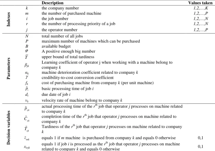
Table 1. Parameters and decision variables

Description Values taken

In

d

ex

es

k the company number 1,2,…,K

m the number of purchased machine 1,2,…,P

i the job number 1,2,…,N

r the number of processing priority of a job 1,2,…,N

j the operator number 1,2,…,P

P a ra m et er s

N total number of all jobs

P maximum number of machines which can be purchased B available budget

ϕ A positive enough big number T upper bound of total tardiness

βjk

Learning coefficient of operator j when working with a machine belong to company k

αk machine deterioration coefficient related to company k

γ credibility-to-cost conversion coefficient

fk cost of purchasing machine from company k (per unit machine)

i

p% basic processing time of job i di due date of job i

vk velocity rate of machine belong to company k

D ec is io n v a ri a b le

s p%rjk

actual processing time of the rth job that operator j processes on machine related to company k

rjk

C% completion time of the r

th _{job that operator j processes on machine related to}

company k

rjk

T% Tardiness of the r

th

job that operator j processes on machine related to company k

mk

z equals 1 if m machine is purchased from company k and equals 0 otherwise 0,1 xirjk

equals 1 if job i is processed as the rth job that operator j processes on machine

related to company k and equals 0 otherwise 0,1

Accordingly, the two-stage model is defined as below:

2SFSP model:

(

)

(

)

_k( , )

k

m k k mk

Min ∑ ∑ m×f z −γE Q z ξ (4) Subject to:

1

k

m mk

z =

∑ ∑ (5)

(

)

(

)

m z P

m f z B

× ≤

× ≤

∑ ∑

∑ ∑

{ }

mk

20

Where

{

}

N m r j

k rjk

Q z ξ Cr T T

= =

= ∑ ∑% ≤ ₍₈₎

Subject to:

1, 0

1, 2,..., and 1, 2,..., 0 1, 2,...,

rjk r jk rjk jk

C C p for r N j m

C for j m

−

= + = =

= =

% % _%

% (9)

(10)

(

)

(

)

1 1, 2,..., and 1, 2,...,

N N

i

rjk irjk rjk irjk

i i

T ϕ x C d x for r N j m

= =

+ −∑ ≥ % −∑ × = =

% ₍₁₁₎

1 1 1 N m irjk r j x i = = = ∀

∑ ∑ (12)

1 , 1,

1

1 1, 2,..., and 1, 2,...,

1, 2,..., 1 and 1, 2,..., , ( 1,..., ), ( )

N irjk i

N I r jk irjk

i

x for r N j m

x x for r N j m I N i I

=

+ ₌

≤ = =

≤ = − = = ≠

∑

∑

{ }

, , 0

0,1

rjk rjk rjk irjk

p C T

x ≥ ∈ % % % (14) In the above model, equation (4) is the objective function for the first stage by which the costs imposed on a system is minimized, consisting of deterministic machine purchase costs and the average of stochastic costs associated with job schedules. Constraint (5) requires that machines must be purchased only from a single company, while constraint (6) defines a maximum number of P machines to be purchased. In the other word, this is a constraint for the capacity of a workshop. Also, it states that machine purchase costs should not be exceeded from the available budget. Constraint (7) specifies a binary variable for the first stage. Equation (8) is to maximize credibility of the total tardiness being less than a predetermined value. Equation (9) calculates the completion time of the rth job processed by operator j on a machine belonged to Company k. However, Equation (10) determined the actual processing time of the rth job by operator j on the machine from Company k. This equation makes it clear that by increasing r, the effect of deterioration increases on each job, thereby increasing processing time. Further, the learning effect plays its role to reduce processing time on a job. Equation (11) calculates the tardiness value of the rth job processed by operator j on the machine from Company k. If no job is assigned to the priority r, then this constraint is satisfied for all

rjk

T% , so T%_rjkequals zero. Constraint (12) necessitates the assignment of each job only and only to one

priority from a given operator. Constraints (13) are designed to check whether only one job and no more is assigned to each priority from one operator and there is no idle time for operators. In this line, if a job is assigned to one priority from an operator, no more jobs could be assigned to that priority of the operator, and also one job must be processed in the previous priority. Finally, constraint (14) defines the decision variables.

3-3- Crisp model based dependent-chance programming

This section deals with the conversion of the two-stage fuzzy programming model from the last section to a deterministic model by using the DCP approach. This approach was first developed by Peng and Liu (2004)and its main idea is to maximize credibility of main objective function of problem being less from a predetermined value. This model defines a variable to calculate the maximum credibility of the objective function. The general DCP model is described as follow:

{

}

max

( , )

. :

( )

( )

Cr f x

r

s t

g x

a

g

b

ξ

ξ

≤

≤

′

≤

%

%

( ( 1) jk) 1, 2,..., and 1, 2,...,

N

i

rjk irjk k

i k

p x p r r for r N j m

v β α =  _{ } = _{ } × _ + × − _× _ = = ∑  % %

21

With respect to equation (3), the crisped model of the problem is defined as follows:

Crisp model:

(

)

(

)

_k( )

k

m k k mk

Min ∑ ∑ m×f z −γE Q z (15)

Subject to: 1

k

m mk

z =

∑ ∑ (16)

(

)

(

)

m z P

m f z B

× ≤

× ≤

∑ ∑

∑ ∑

{ }

mk

z ∈ (18) Where

( ) max

k

Q z = λ (19)

Subject to:

(2) (3)

1 1 1 1

(2 2 )N m _rjk (2 1)N m _rjk

r j r j

T λ T λ T

= = = =

≥ −

∑∑

∑∑

(

)

(

)

( 2) ( 2) ( 2) ( 2)

1, 0

(3) (3) (3) (3)

1, 0

0 1, 2,..., and 1, 2,..., 0 1, 2,..., and 1, 2,...,

rjk r jk rjk jk rjk r jk rjk jk

C C p C for r N j m

C C p C for r N j m

− −

= + = = =

= + = = = (21)

(22)

(

)

(

)

(

)

(

)

( 2 ) ( 2 )

1 1

(3) (3)

1 1

1 1, 2,..., and 1, 2,..., 1 1, 2,..., and 1, 2,...,

N N

i

rjk irjk rjk irjk

i i

N N

i

rjk irjk rjk irjk

i i

T x C d x for r N j m

T x C d x for r N j m

ϕ ϕ = = = = + − ≥ − × = = + − ≥ − × = = ∑ ∑ ∑ ∑ (23) 1 1 1 N m irjk r j x i = = = ∀

∑ ∑

1 1, 2,..., and 1, 2,...,

1, 2,..., 1 and 1, 2,..., , ( 1,..., ), ( )

N irjk i

N I r jk irjk

i

x for r N j m

x x for r N j m I N i I

= + = ≤ = = ≤ = − = = ≠

∑

∑

{ }

( 2) (3) ( 2) (3)

, , , 0

0.5 0,1

rjk rjk rjk rjk

irjk

C C T T

x λ ≥ > ∈ (26)

For the above model, (3)

rjk

T shows the right hand value of the fuzzy number related toT%_rjk. Equation

(19) maximizes the credibility level of the objective function. This value is determined according to constraint (20). Constraints (21), (22) and (23) calculate the completion time, actual processing time, and tardiness value for the rth job of Operator j for the middle and right-side value of the related fuzzy numbers. Other constraints are defined as before.

3-4- Solution procedure

The Crisped model at the last section is very complex. The solution of this model requires solving the model at the second stage dealing with the schedules of jobs on machines for all feasible responses

( 2) ( 2)

1

(3) (3)

1

1

( ( 1) ) 1, 2,..., and 1, 2,...,

1

( ( 1) ) 1, 2,..., and 1, 2,...,

jk jk

N

i

rjk irjk k

i k

N

i

rjk irjk k

i k

p x p r r for r N j m

v

p x p r r for r N j m

v β β α α = =  _{ } = _{ } × _ + × − _× _ = =    _{ } = _{ } × _ + × − _× _ = =  

∑

∑

22

generated by the first stage relating to machine purchases. The optimal solution is the best response obtained at this process. The formal definition of the process is given as below:

Set best solution=infinite, For k=1 to K do

For m=1 to min ,

k

B P _f

 

 

  do

Solve the second stage model,

If this solution is better than the best solution so far then Best solution ← this solution,

End do, End do,

Return best solution.

4- Branch and bound algorithm

4-1- Structural features

Proposition 1. When the company type determined, an optimal scheduling is achieved for the

problem of1D LE,

∑

parameters are deterministic, based on the SPT rule.

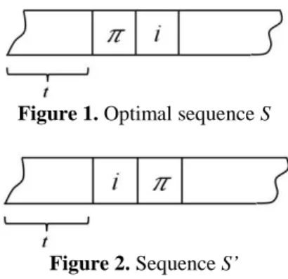
Proof. Proof by contradiction; Consider sequence S (figure 1) as the optimal scheduling of jobs on a

machine. If the SPT rule is false, so there must be at least two jobs such as i and π that for which pi<pπ

is satisfied and π is on the priority rand i is on the priority r+1, respectively. Now, consider the

sequence S’ (figure 2) where the two jobs i and π are swapped. Obviously, there is no change in the

sum of completion times for those jobs before and after this pair. So, it would be enough to compare the sum of completion times resulted from such replacement. Since k and j are determined and

constant, therefore, the proof uses α and β, instead of, αk and βjk.

Figure 1. Optimal sequence S

Figure 2. Sequence S’

Suppose

C

C

C

C

completion times of jobs π and I in sequence S’, respectively. Then we have:

(

)

(

)

s

C_π = +t p_π+ × −α r ×rβ = +t p r_π β +αrβ r−

(

)

s s

i i i

C =C_π + p + × × +α r r β = +t p r_π β+αrβ r− +p r+ β +α r+ βr

(

)

s

i i i

C′ = +t p + × −α r ×rβ = +t p rβ +αrβ r−

(

)

s s

i i

C_π′ =C′+ p_π + × × +α r r β = +t p rβ +αrβ r− +p r_π + β+α r+ βr

(

)

2 2 ( 1) ( 1) ( 1)

s s

i i

C_π C t p r_π β αrβ r p r β α r βr

⇒ + = + + − + + + +

(

)

2 2 ( 1) ( 1) ( 1)

s s

i i

C′ C_π′ t p rβ αrβ r p r_π β α r βr

⇒ _{+ = + + − + + + +}

Sinceβ <0, then (r+1)β <rβ always holds. Now, the sum of completion times in sequence S’is

23

(

) (

)

(

) (

)

(

)

( 1) 2

( 1)

2 0

i i

i

s s s s

i i

r

C C C C p p p p

r r

p p

r

π π

π

β

π π β

β β

′ ′  + 

⇒ _{+ − + = − − −  }

 

 ₊ 

= −  − >

 

We have therefore reached a contradiction and thus it is proven that the proposition holds true.□

Proposition 2. For the problem of scheduling jobs on a single-machine to minimizing the total

tardiness where the effects of deteriorating jobs and learning are both position-based with

deterministic parameters, the value of

{

}

[ ] [ ]

max _{r r} , 0

r C −d

∑ is always considered to be a lower bound.

[ ]r

C is the completion time of a job in the position r, when job ordering is based on SPT rule. And, If

due dates are sorted by the earliest due date (EDD) rule, thend_{[ ]r} is the due date of the rth.

Proof. Kondakci et al. (1994) showed that for a single-machine scheduling problem to minimizing the

total tardiness, the lower bound equals max

{

}

r C −d

∑ , where C_{[ ]r} is the completion time of the

rth job, if jobs are ordered with the shortest processing time (SPT) rule. Further, d_{[ ]r} is the due date of

the rth, when due dates are set by the earliest due date (EDD) rule. □

4-2- Branch and bound scheme

First, the B & B algorithm is used to determine the type of company and the number of machines purchased. Note that the number of machines purchased from the company k must be less than

min ,

k

B P

f

 

 

 . With a given number of machines, then, a parallel machine scheduling problem is

solved for the related node through the B& B algorithm. In order to solve such problem, this algorithm has an m-stage structure (m denotes the number of machines (operator)). Every stage forms the nodes allocated to a job by one operator. At each stage, a maximum of N-level can be developed (N denotes the number of jobs); meaning, the first priority of an operator gets the first level, the

second priority at the second level, and so on. The nth level represents the nth priority. In this structure,

the indexes of each stage and level are denoted by J and I, respectively. At the root, all jobs are first

placed on the set of unscheduled jobs, US. The number of jobs placed on US is shown by nus. At this

node, the stage number is considered equal to 1 (J= 1), it means that scheduling is first to be

performed by Operator 1. At the first level, the number of nodes is n_US+1; where n_USrepresents the

number of nodes generated for unscheduled jobs and called "Active nodes", and 1 node specifies non allocation of jobs to this level of the same operator, which is represented by 0 and called a "Zero

node". If a job is allocated to operator 1, then one more level is generated for that operator, (I = I +1),

and the job assigned to priority 1 of operator 1 is eliminated from US. However, if no job is allocated to operator 1, then the stage number is updated; (J = J +1). So, scheduling of jobs by operator 2 will be checked. This process continues until the set of US is empty. In other words, all jobs are scheduled for operators.

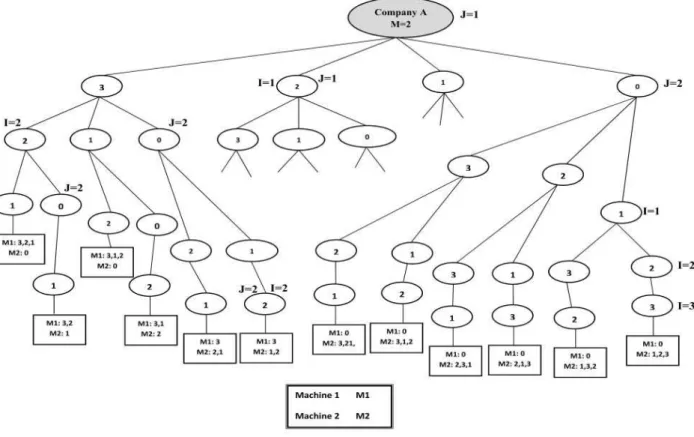
Figure 3 presents the B&B tree structure where a maximum of three machines can be purchased from

Companies A and B., assuming thatmin ,

k

B

P P

f

 

=

 

  . Then, each leaf of the tree develops a B&B

algorithm in order to solve the parallel machine scheduling problem. Figure 4 provides an uncompleted representation for the B&B algorithm when there are three jobs and two machines purchased from the leaf which is selected as company A.

24

Figure 3. Selection of companies by B&B

Figure 4.General scheme of B&B algorithm to achieve the sequence 4-3- Fathoming and backtracking

A node is fathomed if:

1. It is a leaf node; it means all the jobs are scheduled

2. The associated total tardiness lower bound for the node is equal or larger than upper bound

While a node is fathomed, backtracking happens. If there is no node with a nonempty US set, then the process of branching is terminated and the upper bound of that time would be considered as the optimal solution.

25 4-4- Lower bounds

The efficiency of a B&B algorithm is strictly dependent on the lower bounds of each node. In order to compute a lower bound for total tardiness, Azizoglu and Kirca (1998) have addressed that optimal solution of total tardiness parallel machine scheduling with preemption is always a lower bound for its non-preemptive version. So it can be assumed that each job is equally distributed among m machines, and under this assumption, the parallel machine can be changed to a single machine scheduling with

processing times of Pi( )k m . As a result for a partial scheduling of S, a lower bound for total tardiness

can be developed according to proposition 2. Equations (27) and (28) show the computation of T(LB), i.e. lower bound of total tardiness.

( 2) (3)

2 2

( ) (2 2 ) _LB (2 1) _LB

T LB = − λ T + λ − T (27)

{

}

{

(

{

}

)

}

{

}

{

(

{

}

)

}

( 2) ( 2) ( 2) ( 2) ( 2) ( 2)

(3) (3) (1) (3) (3) (1)

[ ] [ ]

[ ] [ ]

max , 0 max min ( ) , 0 max , 0 max min ( ) , 0

r S j r S

r S j r S

rj rj j j

LB r r

rj rj j j

LB r r

T C d C s C d

T C d C s C d

∈ ∉

∈ ∉

= − + + −

= − + + −

∑ ∑ ∑

∑ ∑ ∑

(28)

In equation (27), a credibility approach is used for facing the fuzzy objective. Equation (28) computes lower bound of total tardiness for the middle and right values of fuzzy triangular number. In this equation Crj( )k is the k

th

component of fuzzy completion time of scheduled job in the position r on machine j, and drj( )k is the k

th

component of fuzzy due date of the scheduled job in position r on

machine j. C( )jk is the k

th

component of the largest fuzzy completion time of set S on machine j. C_{[ ]}( )rk is

the kth component of the rth fuzzy completion time according to sequence resulted from SPT rule for

the unscheduled jobs with basic processing times of Pi( )k mActive and learning coefficient of

{ }

min β_jk (an optimistic view for total tardiness). Finally,d_{[ ]}( )rk is the k

th

component of the fuzzy due dates of the unscheduled jobs sorted by EDD rule. In equation (28), the first part computes total tardiness of scheduled jobs. In the second part it is assumed that all the machines are again available

at timemin_j

{

( )

}

preemption is allowed.

5- Genetic algorithm

In the class of NP-hard problems, the complexity of solution space can make it difficult to obtain a real solution by precise optimization techniques and/or they take long time to find solutions. This is why the current study adopts an approach based on a meta-heuristic algorithm. As an optimization method inspired from natural evolution, the genetic algorithm was first introduced by Holland et al. (1975). Later, this process was extended by several scholars such as Goldberg (1989) and Davis (1991). To apply the GA, this paper uses a priority-based approach, where jobs are assigned priorities and scheduled according to their priorities.

A Genetic Algorithm (GA) begins with a set of chromosomes known as a primary response. Each chromosome is assigned an objective function value and this is called the fitness value. The better fitness values the chromosomes have, the more chances to survive and reproduce they have. Defined as an initial population, chromosomes can be constructed by using different methods such as random generation, heuristics, and so on. The next step is the creation of a mechanism to select parents of new generations. Through crossover and mutation operators, the selected parents can generate new children to be a replacement for the old ones. The algorithm continues until a termination criterion is satisfied, like number of repetition or when there is no repetition with improvement.

5-1- Representation

In this section to achieve a feasible solution, two parts A and B were used. Part A determines the assignment of a given job to a certain operator, while Part B specifies the schedule for jobs (priorities) to each operator (machine).In Part A, an integer is randomly generated in {1, …, M} for the number of jobs (N). Accordingly, for Part B, random numbers are generated between zero and 1. Each job is

26

divided by the square root of the sum of the squares of the numbers generated, and then the final numbers are arranged in ascending order when the smallest in Part B is ranked as the first and the largest is assigned N.

To make the statement above, see figure 5. In Company 1, for example, with 3 machines and 10 jobs, (k = 1, N= 10, M=3), the graph of chromosome can be represented as below:

Figure 5.Diagrammatic representations of chromosomes

Regarding the above figure and Part A, it is evident that the set of jobs 3, 4, and 10 are to be processed by the operator 1; while the jobs numbers 1, 5 and 9 and also the job numbers 2, 6, 7 and 8 are processed by operators 2 and 3, respectively. Job orders are determined by part B. So, a description of the job scheduling and resource allocation will be as the following: operator 1 (on with machine 1) is responsible for processing jobs 4, 3 and 10, respectively. Operator 2 (on machine 2) is to process jobs 9, 1 and 5; and operator 3 (on machine 3) process jobs 2, 6, 8, and 7.

5-2- Generation

In order to select members as the parents of a new generation, a technique named as the roulette

wheels is used and select Pc % of population as parent. Then, crossing and mutation operators are

employed for the selected members. For each substring, the operators perform individually. A "one-point" crossing operator is used for chromosomes. It should be noted that diversity of genes must be

followed for the sequence substring of children. Each child can be mutated by the chance of Pm%. A

"random derangement" mutation operator is provided for chromosomes. Having developed a new

generation and combined with old one, Np better chromosomes are transferred into the next

generation. Reaching a pre-determined maximum number for iterations (Ng) meets the termination

criterion. So, the algorithm ends and the best solution is provided.

5-3- Parameters tuning

Here, the following values are suggested for the parameters required in the GA after running of this algorithm for some of benchmark instances:

The Probability of Crossover (Pc) and the Probability of Mutation (Pm), each at three levels, are0.8,

0.85 and, 0.9; and 0.03, 0.06 and, 0.09. The number of initial population (Np) and the number of

generation (Ng) are in three levels of 50, 100 and 150; and 300, 400 and, 500, respectively.

By comparing the experimental results and the changes to arguments (default parameter values), the best values are given as below:

PC = 0.85, Pm= 0.09, NP = 150 and, Ng= 400.

6- Computational results

In this section, a variety of examples is randomly generated in order to compare and evaluate the proposed methods. The linear scheduling model is solved by the CPLEX solver, running on a system with Intel Core i7 3.1 GHz CPU and 8 GB of RAM configuration. The B&B algorithm and GA are also coded in C# and run on the same system. To generate random examples, a basic processing time is achieved from uniformly distribution function on [10, 50]. Due dates, velocity rate of machines from the kth company, and purchasing costs for a new machine are obtained from uniform distribution

27

functions on 5, 15 n

P

×













[

]

αk are determined on [-0.4, -0.1] and [0.1, 0.4]. Furthermore, the value of γ is equal to 1000. In order

to obtain a feasible value for budget, the uniform distribution function on

[

]

Since Tcan be calculated only when the problem is solved, feasible numbers for this parameter are

achieved through training different values. Tables 2 and 3 show the computational results for the mathematical programming model for P=2 and P=3, respectively. In these tables, the number of current companies and also the number of jobs are represented for each example. Also, the running times are provided per seconds. Based on the results, the running time increases as the numbers of job and machine increase; however, although increases in the number of jobs lead to a higher running time (similar to an exponential growth) comparing increases in the number of companies. These tables show that for P=3, the mathematical model only solves small cases with less than 11 jobs in a logical running time (here, 10000 Sec). Therefore, it can be predicted that if P>3, then the mathematical model will not be able to provide solutions for very small-sized problems.

Table 2. Results for MILP model for P=2

# of Company # of jobs Avg. CPU running times (Sec.)

1 5 08.3

7 54.5

9 307.8

11 1691.1

13 2905.8

2 5 15.6

7 125.4

9 653.5

11 3015.7

3 5 27.2

7 139.6

9 879.0

11 4707.3

Table 3. Results for MILP model for P=3

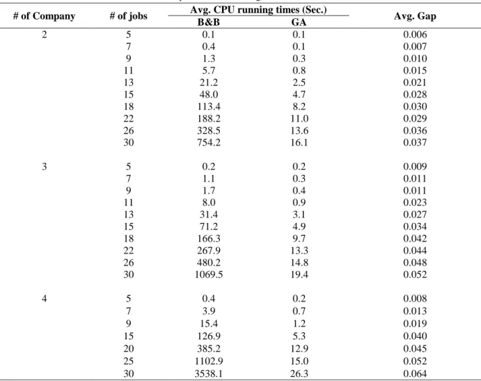
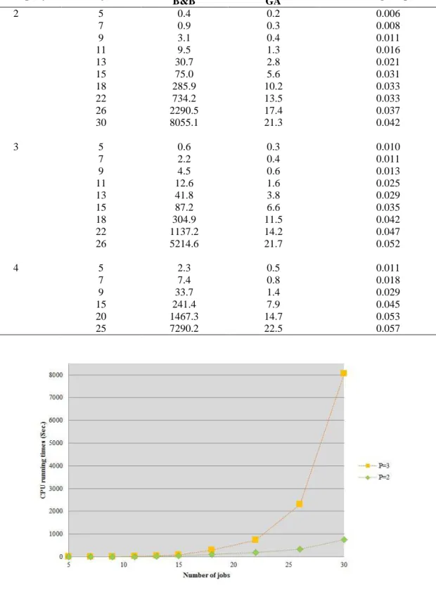
Tables 4 and 5 presents the comparative results of the B&B algorithm and GA for P=2 and P= 3, respectively. As seen, the running time of B&B algorithm increases as the numbers of job and company increase, although increases in the number of jobs lead to a higher running time (similar to an exponential growth) comparing increases in the number of companies. Like the mathematical model proposed, the B&B algorithm is sensitive to P-value and hence for P=3 the running time is greater than for P=2. This result is shown in figure 6. Rather, the GA approach has a polynomial running time and this character holds both when the numbers of job and machine increase. Moreover, an increased P yields to small changes in the graph of run time as seen in figure 7. The value of GA error from the optimum obtained by the B&B algorithm can be also resulted from tables 4 and 5. As found, any increases in the number of jobs, number of machines, and also in the P all lead to

# of Company # of jobs Avg. CPU running times (Sec.)

1 5 24.6

7 198.4

9 1323.7

11 5748.0

2 5 46.9

7 412.5

9 2664.1

28

increasing errors from the final solution. However, it seems that due to making the solution dimensions larger, the increased number of jobs has much more significant effects on errors from the resultant solutions.

Table 4. Comparison of B&B algorithm and GA for P=2

# of Company # of jobs Avg. CPU running times (Sec.) Avg. Gap B&B GA

2 5 0.1 0.1 0.006

7 0.4 0.1 0.007

9 1.3 0.3 0.010

11 5.7 0.8 0.015

13 21.2 2.5 0.021

15 48.0 4.7 0.028

18 113.4 8.2 0.030

22 188.2 11.0 0.029

26 328.5 13.6 0.036

30 754.2 16.1 0.037

3 5 0.2 0.2 0.009

7 1.1 0.3 0.011

9 1.7 0.4 0.011

11 8.0 0.9 0.023

13 31.4 3.1 0.027

15 71.2 4.9 0.034

18 166.3 9.7 0.042

22 267.9 13.3 0.044

26 480.2 14.8 0.048

30 1069.5 19.4 0.052

4 5 0.4 0.2 0.008

7 3.9 0.7 0.013

9 15.4 1.2 0.019

15 126.9 5.3 0.040

20 385.2 12.9 0.045

25 1102.9 15.0 0.052

29

Table 5. Comparison of B&B algorithm and GA for P=3

# of Company # of jobs Avg. CPU running times (Sec.) Avg. Gap B&B GA

2 5 0.4 0.2 0.006

7 0.9 0.3 0.008

9 3.1 0.4 0.011

11 9.5 1.3 0.016

13 30.7 2.8 0.021

15 75.0 5.6 0.031

18 285.9 10.2 0.033

22 734.2 13.5 0.033

26 2290.5 17.4 0.037

30 8055.1 21.3 0.042

3 5 0.6 0.3 0.010

7 2.2 0.4 0.011

9 4.5 0.6 0.013

11 12.6 1.6 0.025

13 41.8 3.8 0.029

15 87.2 6.6 0.035

18 304.9 11.5 0.042

22 1137.2 14.2 0.047

26 5214.6 21.7 0.052

4 5 2.3 0.5 0.011

7 7.4 0.8 0.018

9 33.7 1.4 0.029

15 241.4 7.9 0.045

20 1467.3 14.7 0.053

25 7290.2 22.5 0.057

30

Figure 7.Effects of number of jobs on running time by GA for two companies.

7- Conclusion

Decision makers in manufacturing environments are required to take into account both strategic and operational issues. Considering different practical constraints (e.g., budget constraints, inventory space, etc.), they typically make strategic decisions first to minimize the establishment costs. In the next step, the operational decisions are determined based on due dates for delivery time so that the customer satisfaction is enhanced. The current paper presented a two-stage fuzzy-stochastic programming model to determine the number of machines in production environments and order scheduling, with fuzzy processing times of a job where machine deterioration and learning effects were both examined. At the first stage, the problem aimed to minimize purchasing costs for new machinery. Accordingly at the next stage, orders were scheduled with the objective function of minimizing total tardiness. For this stage, the model was defuzzifed using dependent-chance programming. Since it was an NP-hard problem, a branch and bound (B&B) algorithm was developed and effective lower bounds were obtained. Further, a genetic algorithm (GA) meta-heuristic approach was addressed to solve large-sized problems.

The computational results revealed that the developed methods (i.e. linear mathematical programming model and B&B algorithm) are very sensitive to the number of jobs and value of P, and that their running times increase exponentially as these two elements increase. However, the proposed GA heuristic is much less sensitive to the number of jobs and the values of P, and it has a polynomial solution time. The computational results also indicated the high efficiency of GA to arrive at global optimum solutions. The future research can investigate the performance of the proposed approach in tackling other problems such as project scheduling. Another direction for future research can be the incorporation of the production planning decisions into the developed model. Additionally, comparing the behavior of the proposed dependent-chance programming method with other uncertainty programming approaches including robust optimization methods would lead to more managerial insights.

31 References

Al-Khamis, T. & R. M’Hallah (2011) A two-stage stochastic programming model for the parallel machine scheduling problem with machine capacity. Computers & Operations Research, 38, 1747– 1759.

Baptiste, P., J. Carlier, A. Kononov, M. Queyranne, S. Sevastyanov & M. Sviridenko (2012) Integer preemptive scheduling on parallel machines. Operations Research Letters, 40, 440–444.

Bozorgirad, M. A. & R. Logendran (2012) Sequence-dependent group scheduling problem on unrelated-parallel machines. Expert Systems with Applications, 39, 9021–9030.

Fanjul-Peyro, L., F. Perea & R. Ruiz (2017) MIP models and matheuristics for the unrelated parallel machine scheduling problem with additional resources. European Journal of Operational Research. Gerstl, E. & G. Mosheiov (2012) Scheduling on parallel identical machines with job-rejection and position-dependent processing times. Information Processing Letters, 112, 743–747.

Gharehgozli, A. H., R. Tavakkoli-Moghaddam & N. Zaerpour (2009) A fuzzy-mixed-integer goal programming model for a parallel-machine scheduling problem with sequence-dependent setup times and release dates. Robotics and Computer-Integrated Manufacturing, 25, 853–859.

Ji, M. & T. C. E. Cheng (2008) Parallel-machine scheduling with simple linear deterioration to minimize total completion time. European Journal of Operational Research 188, 342–347.

Joo, C. M. & B. S. Kim (2015) Hybrid genetic algorithms with dispatching rules for unrelated parallel machine scheduling with setup time and production availability. Computers & Industrial Engineering, 85, 102-109.

Kondakci, S., Ö. Kirca & M. Azizoǧlu (1994) An efficient algorithm for the single machine tardiness

problem. International journal of production economics, 36, 213-219. Lee, K. H. 2006. First course on fuzzy theory and applications. Springer.

Lee, W.-C., M.-C. Chuang & W.-C. Yeh (2012) Uniform parallel-machine scheduling to minimize makespan with position-based learning curves. Computers & Industrial Engineering, 63, 813–818. Liao, L. W. & G. J. Sheen (2008) Parallel Machine Scheduling with Machine Availability and Eligibility Constraints. European Journal of Operation Research, 184, 458-467.

Liu, B. & Y.-K. Liu (2002) Expected value of fuzzy variable and fuzzy expected value models. IEEE

Transactions on Fuzzy Systems, 10, 445–450.

Liu, M. (2013) Parallel-machine scheduling with past-sequence-dependent delivery times and learning effect. Applied Mathematical Modelling, 37, 9630–9633.

Liu, M., F. Zheng, S. Wang & Y. Xu (2013) Approximation algorithms for parallel machine scheduling with linear deterioration. Theoretical Computer Science, 497, 108–111.

Mazdeh, M. M., F. Zaerpour, A. Zareei & A. Hajinezhad (2010) Parallel machines scheduling to minimize job tardiness and machine deteriorating cost with deteriorating jobs. Applied Mathematical

Modelling, 34, 1498–1510.

Mosheiov, G. (2001) Scheduling problems with a learning effect. European Journal of Operation

32

Peng, J. & B. Liu (2004) Parallel machine scheduling models with fuzzy processing times.

Information Sciences, 166, 49–66.

Prot, D., O. Bellenguez-Morineau & C. Lahlou (2013) New complexity results for parallel identical machine scheduling problems with preemption, release dates and regular criteria. European Journal

of Operational Research, 231, 282–287.

Rodriguez, F. J., M. Lozano, C. Blum & C. Garcı´a-Martı´nez (2013) An iterated greedy algorithm for the large-scale unrelated parallel machines scheduling problem. Computers & Operations Research, 40, 1829–1841.

Rostami, M., A. E. Pilerood & M. M. Mazdeh (2015) Multi-objective parallel machine scheduling problem with job deterioration and learning effect under fuzzy environment. Computers & Industrial

Engineering, 85, 206-215.

Ruiz-Torres, A. J., G. Paletta & E. Pe´rez (2013) Parallel machine scheduling to minimize the makespan with sequence dependent deteriorating effects. Computers & Operations Research, 40, 2051–2061.

Sarıçiçek, I. & C. Çelik (2011) Two meta-heuristics for parallel machine scheduling with job splitting to minimize total tardiness. Applied Mathematical Modelling, 35, 4117–4126.

Shen, L., D. Wang & X.-Y. Wang (2013) Parallel-machine scheduling with non-simultaneous machine available time. Applied Mathematical Modelling, 37, 5227–5232.

Tian, W. & C. S. Yeo (2015) Minimizing total busy time in offline parallel scheduling with application to energy efficiency in cloud computing. Concurrency and Computation: Practice and

Experience, 27, 2470-2488.

Toksari, M. D. & E. G¨uner (2009) Parallel machine earliness/tardiness scheduling problem under the effects of position based learning and linear/nonlinear deterioration. Computers & Operations

Research, 36, 2394 -- 2417.

Unlu, Y. & S. J. Mason (2010) Evaluation of mixed integer programming formulations for non-preemptive parallel machine scheduling problems. Computers & Industrial Engineering, 58, 785–800. Vallada, E. & R. Ruiz (2011) A genetic algorithm for the unrelated parallel machine scheduling problem with sequence dependent setup times. European Journal of Operational Research, 211, 612– 622.

Yeh, W.-C., P.-J. Lai, W.-C. Lee & M.-C. Chuang (2013) Parallel-machine scheduling to minimize makespan with fuzzy processing times and learning effects. Information Sciences.

Zadeh, L. A. (1965) Fuzzy sets. Inf. Control, 8, 338–353.

Zhang, M. & C. Luo (2013) Parallel-machine scheduling with deteriorating jobs, rejection and a fixed non-availability interval. Applied Mathematics and Computation, 224, 405–411.

Zhu, H. & J. Zhang (2009) A credibility-based fuzzy programming model for APP problem. In