HIGH-DIMENSIONAL JOINT MODEL FOR
LONGITUDINAL BINARY OUTCOME
B.M. DANSU1, O.E. ASIRIBO2 AND S.O. SAM-WOBO31,2Department of Statistics,
3Department of Biological Sciences,
Federal University of Agriculture, Abeokuta. Postcode 110001. Nigeria.
*Corresponding author: [email protected]
2004).
Longitudinal data are very common in bio-medical research and clinical trials, where the characteristic or some measurement of a per-son such as the status of a disease of one person, evolves or develops over time. Existing statistical methods such as logistic and multinomial logistic models for analyz-ing longitudinal discrete data had been pri-marily developed for multivariate data col-lected at a single time point, such methods may be inappropriate for analyzing
multivari-ABSTRACT
Binary outcomes are often collected in clinical and epidemiological studies to investigate the evolution of some outcomes over time. In studies with two or more binary outcomes, research questions often revolve around the joint evolution of the binary outcomes over time. However, independently modelling the evolution of each outcome variable ignores the correlation among the variables. Although general-ized mixed models have been proposed to model the joint evolution of binary outcome variables over time, the estimation of the corresponding regression coefficients and covariance parameters may be computationally difficult as the number of outcome variables increases. In this study, we investigate the use of a pairwise generalized mixed models approach based pseudo-likelihood theory, in which all possible bivariate models are fitted, to estimate the parameters of a multivariate longitudinal binary data and compared it with univariate models. This methodology is illustrated using data from a longi-tudinal study of the prevalence of four ailments in 200 children in the south-western part of Nigeria. This methodology is shown to be computationally easy and beneficial over the conventional multivari-ate generalized model methods. It is also advantageous over univarimultivari-ate generalized mixed-effects models as it incorporates the modeling. This research provides applied researchers with alter-native tools to investigate the joint evolution of binary outcomes over time.
Keywords: High-dimensional, joint model, Pseudo-likelihood, Mixed outcomes, Correlated data
INTRODUCTION
Longitudinal studies seek to investigate change over time for study participants who are measured at two or more occasions. In the health sciences, longitudinal data arise in clinical and epidemiological studies (Charles & Davis, 2002). Longitudinal studies are useful for describing changes over time for groups, as well as subject specific variation in the magnitude of change. In addition, these studies are useful for identifying vari-ables associated with change and under-standing how changes in outcomes are re-lated to one another (Fieuws & Verbeke,
Journal of Natural Sciences, Engineering
and Technology
ISSN:
Print - 2277 - 0593 Online - 2315 - 7461
ate longitudinal data because they do not account for the correlation among the out-come variables. Statistical methods for ana-lyzing multivariate longitudinal binary data have been proposed based on generalized mixed-effects models (Molenbergs, Fiuews and Verbeeke, 2000), in which the multi-variate model parameters are estimated from a series of bivariate mixed-effects models for all possible pairs of the outcome variables. In addition, statistical methods for analyzing these data are not readily available in existing statistical software packages. The motivation for this research came from computational problem in using full likeli-hood when there is increase in the number of outcome especially in longitudinal study of health data. Clinicians have long relied on statistical methods that model the longi-tudinal change in one outcome variable at a time. However, multiple outcomes are com-mon in longitudinal study especially in health data where the presence of one ease often increases the risk of other dis-ease. In such case longitudinal methods that jointly model the evolution of these diseases over time are most appropriate.
The overall purpose of this study is to ex-amine multivariate statistical models for longitudinal binary outcomes that include covariate effects and account for correlation among the outcomes. The implementation of these procedures will be demonstrated using data from a longitudinal study of common disease and symptoms in children under five years in south-western Nigeria.
METHODS
Pairwise Modeling
The principal idea is to replace a numeri-cally challenging joint density by an
ap-proximate and simpler function such as the product of ratios of conditional likelihoods of all possible pairs of the outcome variables. For example, when joint density contains a computationally intractable normalizing con-stant, one might calculate a suitable product of conditional density that does not involve such a complicated function. Although this method achieves important computational economies by changing the method of esti-mation, it does not affect the model parame-ters, parameters can be chosen in the same way as with full likelihood, retain their mean-ing, and so on. Estimation of pseudo-likelihood is more attractive than maximum likelihood especially in binary data.
Pairwise fitting approach model
This describes in detail how to estimate all the parameters using pairwise fitting ap-proach. Let p be the number of outcomes that need to be modeled jointly. For this study p is equal to 4. Further, let Yr denote
the rth outcomes, r=1,..., p, and let be the vector of all parameters in the multivariate model (Y1, Y2, …,Yp). The pairwise-fitting approach starts from fitting all p(p-1)/2 bivariate models, that is, all joint models for all possible pairs (Y1, Y2), (Y1, Y3), …, (Y1,
Yp), (Y2, Y3),…, (Y2, Yp),…, (Yp-1, Yp) of the outcomes Y1,Y2,…,Yp. Let the log-likelihood
function corresponding to the pair (r, s) be denoted by l(yr, ys| ), and let be the vector containing all parameters in the bivariate model for pair (r, s).
Let now be the stacked vector combin-ing all p (p − 1)/2 pair-specific parameter vectors . Estimates for the elements in
*
Ψ
rs
Ψ Ψrs
Ψ
rs
are obtained by maximizing each of the
p(p − 1)/2 log-likelihoods l(yr, ys| ) separately. The parameter vectors and
are not equivalent, i.e. some parame-ters in will have a single counterpart in . From here a single estimate for the corresponding parameter in is obtained by averaging all corresponding pair specific estimates in . Indeed, two pair-specific estimates corresponding to two pairwise models with a common outcome are based on overlapping information and hence cor-related. This correlation should also be ac-counted for in the sampling variability of the combined estimates in . However asymptotic standard errors for the parame-ters in , and consequently in can be obtained from pseudo-likelihood ideas.
Inference for all pairs of parameters ( )
In order to draw the inference there is need to take account of variability among
pair-Ψ
rs Ψ
Ψ
*
Ψ
*
Ψ Ψ
*
Ψ
Ψˆ
*
Ψˆ
Ψˆ Ψˆ*
Ψ
specific estimates because standard error cannot be obtained from averaging. Also two pairs of outcomes are expected to be corre-lated and this correlation should be ac-counted for in the sampling variability of the combined estimate in . However, adopt-ing pseudo-likelihood estimation (Bessag, 1975) is to replace the joint likelihood by suitable conditional or marginal densities, this will make evaluation of the product eas-ier rather than complex in the previous methods (Renard, Molenberghs & Geys, 2004). Pairwise approach involves maximiz-ing a set of likelihood separately which is suitable for pseudo-likelihood. The applica-tion of pseudo likelihood methodology is different from most other applications in the sense that the same parameter vector is usu-ally present in different parts of the pseudo likelihood function. Here the set of parame-ters in is treated pair-specific, which allows separate maximization of each term in the pseudo log-likelihood function. Fitting all bivariate models is equivalent to maximizing the function
*
Ψ
rs
Ψ
) (1)
Ψ Ψ) pl(y1i,y2i,...,ypi
pl( l(y ,y )
s r
r s Ψrs
ignoring the fact that some of the vectors have common elements, that is, as-suming that all vectors are completely distinct. The function in Equation (1) can be considered a pseudo-likelihood function, maximization of which leads to so-called pseudo-likelihood estimates with well-known asymptotic statistical properties.
rs
Ψ
rs
Ψ
Finally, estimates for the parameters in can be calculated by taking averages of all available estimates for that specific parame-ter over all pairs which implies that
for an appropriate weight ma-trix . The inference for the elements in
will be based on
*
Ψ
Ψ A Ψˆ* ˆ
A * Ψˆ (2) ) N(0, ) ˆ ( N ) ˆ (
N 1 01
1
0 I I A
I A Ψ A Ψ A Ψ
Ψ* *
Description of the data and analysis
The comparison of statistical methods for analyzing multivariate binary data will be implemented using data from a longitudinal survey conducted in eight different loca-tions in south-western Nigeria. The objec-tive of the survey is to investigate the ef-fects of environmental factors on the preva-lence of common ailments in children un-der five years. In this the ailments studied were cough, malaria, diarrhea, and mumps. It is hypothesized that temperature, good drainage system, availability of good drink-ing water, parent’s educational status, family background, and size of the family are risk factors associated with the prevalence of some of these ailments. These variables are combination of measure of physical envi-ronment, socio-economic, climate and demographic characteristics. The GEN-MOD procedure in SAS Version 9.2 (SAS, 2008) was used to estimate the regression coefficients and the associated standard
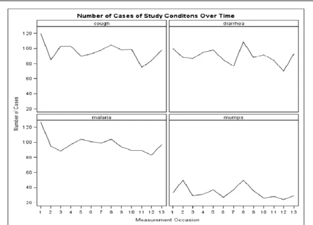
er-rors of marginal model. For the generalized linear mixed model, SAS GLIMMIX proce-dure was used. All analyses focused on de-scribing the factors associated with the evo-lution of the multiple diseases evolve over time. The GENMOD procedure in SAS Version 9.2 (SAS, 2008) was used to estimate the regression coefficients and the associated standard errors of marginal model. For the generalized linear mixed model, SAS GLIM-MIX procedure was used. All analyses fo-cused on describing the factors associated with the evolution of the multiple diseases evolve over time. SAS/IML code was used to combine parameters from all possible bivariate models, and SAS/STAT code to implement bivariate generalized mixed-effects models. Figure 1 below shows occur-rence of each of the four diseases over thir-teen time of visit.
Figure 1: Number of cases studied over time
RESULTS AND DISCUSSION
The study results allow joint analysis of multivariate repeated measures of a relatively high dimension for ease (ability) computational and to identify each model and its strength and limitation. The method is based on fitting bivariate mixed models for all pairs of outcomes. The AIC and BIC were used to measure the goodness of fit, the pairwise AIC and BIC values were smaller than the AIC and BIC of univariate models.However, we have applied a pairwise modelling strategy to obtain parameter estimates of high dimensional GLMMs for binary data. The analysis has illustrated the many advantages of using the pairwise approach in this context. First, the strengths of the random-effects approach for joint
modelling are kept. For example, insight can be gained in the association structure of the outcomes. Also, discarding subjects from the analysis due to missing item scores or con-sidering questionable imputation techniques is not needed. Second, no strong a priori (unidimensionality) assumption about the covariance structure of the random effects needs to be made, thereby avoiding potential biases in the fixed effects estimates. Finally, high dimensional integration problems are avoided. As such, the complicated four-dimensional integration problem in the ap-plication has been eliminated with pseudo likelihood approach.
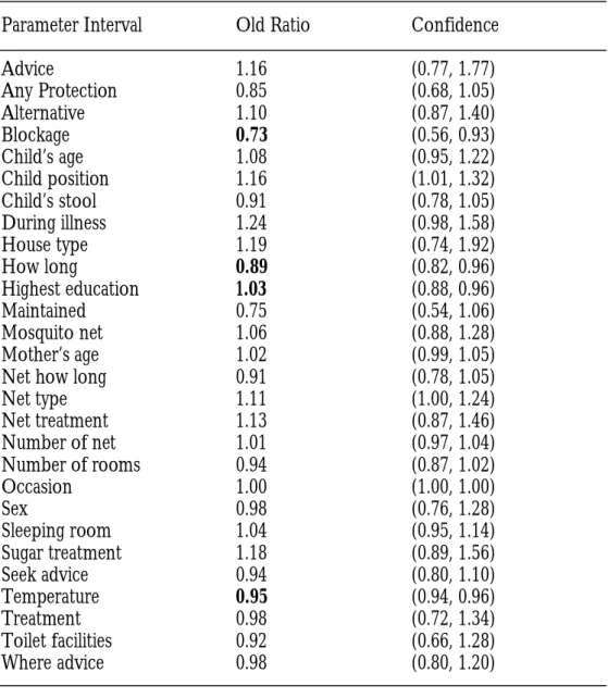
The model results from this study (Table 1) is characterized by outcome-specific fixed, random effects and Pairwise fitting approach (PFA). An important advantage of the PFA
method is that it directly yields unique pa-rameter estimates of the joint model, which is very appealing for inference. This study was particular emphasis on the PFA of
binary outcomes, but the method is in no way restricted to this setting, and can be used for arbitrary combinations of any outcome types.
Table 1: Pairwise fitting model estimates for mixed-effects with 95% confidence intervals
Parameter Interval Old Ratio Confidence
Advice 1.16 (0.77, 1.77)
Any Protection 0.85 (0.68, 1.05)
Alternative 1.10 (0.87, 1.40)
Blockage 0.73 (0.56, 0.93)
Child’s age 1.08 (0.95, 1.22)
Child position 1.16 (1.01, 1.32)
Child’s stool 0.91 (0.78, 1.05)
During illness 1.24 (0.98, 1.58)
House type 1.19 (0.74, 1.92)
How long 0.89 (0.82, 0.96)
Highest education 1.03 (0.88, 0.96)
Maintained 0.75 (0.54, 1.06)
Mosquito net 1.06 (0.88, 1.28)
Mother’s age 1.02 (0.99, 1.05)
Net how long 0.91 (0.78, 1.05)
Net type 1.11 (1.00, 1.24)
Net treatment 1.13 (0.87, 1.46)
Number of net 1.01 (0.97, 1.04)
Number of rooms 0.94 (0.87, 1.02)
Occasion 1.00 (1.00, 1.00)
Sex 0.98 (0.76, 1.28)
Sleeping room 1.04 (0.95, 1.14)
Sugar treatment 1.18 (0.89, 1.56)
Seek advice 0.94 (0.80, 1.10)
Temperature 0.95 (0.94, 0.96)
Treatment 0.98 (0.72, 1.34)
Toilet facilities 0.92 (0.66, 1.28)
Where advice 0.98 (0.80, 1.20)
(Manuscript received: 25th May, 2011; accepted: 27th June, 2011).
REFERENCES
Airy, G.B. 1861. On the Algebraical and
Numerical Theory of Errors of Observation and the Combination of Observations. Lon-don: Macmillan.
Charles, S.D. 2002. Statistical Methods for the
Analysis of Repeated Measurements.
Springer-Verlag New York, Inc.
Fieuws, S., Verbeke, G. 2004. Joint
mod-elling of multivariate longitudinal profiles: pitfalls of the random-effects approach.
Sta-tistics in Medicine, 23: 3093–3104.
Fieuws, S., Verbeke, G., Molenberghs, G. 2007. Random effects models for
multi-variate repeated Measures. Statistical Methods
Medical Research, 16: 387-397
Hideki, O., Knoket, J.D. 1990. A
Com-parative Study of Two Statistical Models for the Analysis of Binary Data from Longitu-dinal Studies. Environmental Health
Perspec-tives, 87: 143-147.
Korn, E.L., Whittemore, A.S. 1979.
Meth-ods of Analyzing Panel Studies of Acute Health Effects of Air Pollution. Biometrics, 35: 795-802.
Laird, N.M., Ware, J.H. 1982.
Random-Effects Models for Longitudinal Data.
Bio-metrics, 38: 963-974.
Fitzmaurice, G.M., Laird, N.M., Ware, J.H. 2004. Applied longitudinal analysis. New
York: John Wiley & Sons.
Molenberghs, G., Verbeke, G. 2006.
Mod-els for Discrete Longitudinal Data. Springer