DOI:10.29252/jirss.19.1.1
Accurate
Inference
for
the
Mean
of
the
Poisson-Exponential
Distribution
WeiLin1,XiangLi2,AugustineWong2
1 Department of Mathematics and Statistics, Thompson Rivers University, 805 TRU Way,
Kamloops, British Columbia, Canada V2C 0C8.
2 Department of Mathematics and Statistics, York University, 4700 Keele Street, Toronto, Ontario,
Canada M3J 1P3.
Received:13/11/2018,Revisionreceived: 27/06/2020,Publishedonline: 28/06/2020
Abstract.Although the random sum distribution has been well-studied in probability
theory, inference for the mean of such distribution is very limited in the literature. In thispaper, two approaches are proposed to obtain inference for the mean of the Poisson-Exponential distribution. Both proposed approaches require the log-likelihood functionofthePoisson-Exponentialdistribution,buttheexactformofthelog-likelihood functionisnotavailable. Anapproximateformofthelog-likelihoodfunctionisthen derived by the saddlepoint method. Inference for the mean of the Poisson-Exponential distributioncaneitherbeobtainedfromthemodifiedsignedlikelihoodrootstatisticor fromtheBartlettcorrectedlikelihoodratiostatistic. Theexplicitformofthemodified signed likelihood root statistic is derived in this paper, and a systematic method to numerically approximate the Bartlett correction factor, hence the Bartlett corrected likelihoodratiostatisticisproposed. Simulationstudiesshowthatbothmethodsare extremely accurate even when the sample size is small.
Keywords. BartlettCorrectionp-valueFunction,SaddlepointApproximation,Signed
Corresponding Author: Wei Lin ([email protected]) Xiang Li ( [email protected])
Augustine Wong ([email protected])
Likelihood Root.
MSC:62E20, 62F03, 62F05, 62F40.
1
Introduction
In probability theory, a compound Poisson distribution is defined byS=PN
i=1Xiwhere Xi is a sequence of identical and independently distributed (iid) random variables andN follows a Poisson distribution with Xi independent ofN. As an example for the motivation of the compound Poisson distribution, let X be the claims that an insurance company has to pay to its clients. The arrival times of these payments, which is a counting process, follow a specific distribution. When the underlying counting process is a Poisson process, and the claims are random variables, then the amount of total claims is a compound Poisson process. The compound Poisson distribution is not only used in actuarial science and insurance for modeling the distribution of total claim, but also used in reliability theory, queuing theory, molecular sequence analysis, etc.
Although the compound Poisson distribution appears in many fields, the explicit distribution ofSis, generally, not available in closed form. Barbour and Chryssaphinou (2001) review and discuss Stein’s method to derive bounds on the error bound in compound Poisson approximation. For the same problem, Bero (2003) uses Kerstan’s method to derive new bounds for the total variation distance. More recently, Barbouret al. (2010) provide an information-theoretic treatment of the problem of approximating the distribution. As well, Alya and Low (2013) derive the approximated density forS
whenX1, . . . ,XN are iid random variables from the Exponential distribution.
This paper is motivated by the previous insurance example. Our aim is to obtain inference for the mean parameter in the compound Poisson distribution with a sum of Exponentially distributed random variables. Specifically, we assume that the amount of a claim, Xi, is Exponentially distributed with mean β and the number of claims, N, is following a Poisson distribution with mean λ. Then S = X1 +· · ·+XN is the aggregate claims generated by the portfolio for the period under study. This specific compound Poisson process is often referred to as the Poisson-Exponential distribution. It is important to note that ifN=0 is realized, thenSmust be zero.
SinceSfollows the Poisson-Exponential distribution, the moment generating
on (mgf) can be obtained as
mS(t) = mNlogmX(t). Hence,E(S) is
ψ=E(S)=E(N)E(X)=λβ .
The main objective of this paper is to obtain inference ofψbased on an observed sample of aggregate claims (s1,s2, . . . ,sk). We are especially interested in the case where sample size,k, is small.
In the literature, there are limited studies on the inference of the Poisson-Exponential distribution. Thmazella et al. (2013) propose a Bayesian inference method for the shape parameter of the newly proposed Poisson-Exponential distribution by using Markov chain Monte Carlo simulation. Ghribi and Masmoudi (2013) introduce the compound Poisson model in the Bayesian network framework and apply implicit inference to this model for learning the parameters of the network. Both are Bayesian methods and pay no attention to the inference of the mean parameter. In this paper, we address the problem of mean parameter inference of the Poisson-Exponential distribution. First, we review the approximation to obtain the density function of S, and hence, the corresponding log-likelihood function. Then two likelihood-based inference approaches are proposed. Finally, we study the performance of the proposed inference methods when sample size is small by simulation studies.
The outline of the rest of the paper is as follows: in Section 2, we review the saddlepoint approximation of the density function ofS. In Section 3, the first-order and third-order likelihood inference methods are reviewed and specifically applied to obtaining inference of the Poisson-Exponential distribution. Moreover, an algorithm to estimate the Bartlett correction factor is proposed in Section 4. To compare the accuracy of the methods discussed in this paper, simulation studies are conducted, results are reported and discussed in Section 5. Further concluding remarks are given in Section 6.
2
Saddlepoint Approximation for the Poisson-Exponential
Di-stribution
LetY1, . . . ,Yn be iid random variables with a known mgfmY(t). By inverting mY(t),
Daniels (1954) proposes using the saddlepoint method to approximate the density
function of ¯Y=Pn
i=1Yi/n. The approximated density function takes the form in below
fY¯( ¯y)=c
n K(2)Y (ˆt)
1/2
expnnhKY(ˆt)−tˆy¯ io
,
where c is the normalizing constant,KY(t) = logmY(t) is the cumulant generation function,
K(Yj)(t)= d jK
Y(t) dtj ,
is the jth derivative of the cumulant generating function, and ˆt is the saddlepoint satisfying KY(1)(ˆt) = y. Moreover, based on this approximated density function and¯ complex integration, Lugannani and Rice (1980) derive the approximated distribution function of ¯Y, which takes the form
FY¯( ¯y)= Φ( ˆw)+φ( ˆw)
1
ˆ w−
1 ˆ u
+O(n−3/2),
whereφ() andΦ() are the density and cumulative distribution functions of the standard normal distribution,
ˆ
w=sgn(ˆt)n2nhtˆy¯−KY(ˆt)io1/2, and uˆ =tˆhnK(2)Y (ˆt)i1/2.
Since there is a singularity point at ˆt =0, Daniels (1987) derives the limiting value of FY¯( ¯y) at the singularity point:
FY¯( ¯y)= 1 2 +
K(3)Y (0)
6
√
2πhKY(2)(0)i3/2
.
Consider the random sum problem withNbeing a Poisson random variable with meanλ, andX1, . . . ,XNbeing iid Exponentially distributed with meanβ. ForN=n,0,
andt,1/β, we have
mN(t)=expnλ(et−1)o, and mX(t)= 1
1−βt.
Therefore, the mgf of the aggregate claims is
mS(t)=mNlogmX(t)=exp (
λ
" 1 1−βt −1
#)
,
and the corresponding cumulant generating function is
KS(t)=logmS(t)=λ "
1 1−βt−1
#
.
By applying the saddlepoint method, Alya and Low (2013) derive the approximated density for the aggregate claimsS,
fS(s)= q c KS(2)(ˆt)
expnKS(ˆt)−tsˆ o, (2.1)
where
K(1)S (t)= λβ
(1−βt)2, K (2) S (t)=
2λβ2
(1−βt)3, (2.2) and ˆtsatisfiesK(1)S (ˆt)=s, which results in
ˆ t= 1
β
1
− λβ
s !1/2
. (2.3)
Based on the approximated density and applying the Lugganni and Rice method, Alya and Low (2013) examine the accuracy of the cumulative distribution of S for givenλandβ. But in practice,λandβare unknown, so is the mean parameter,ψ=λβ. Obtaining inferenceψis of great interest to many insurance companies. However, there is a paucity of literature on this problem. Two inferential methods forψare proposed in the next two sections. The first method derived in Section 3 is based on the third-order likelihood-based method discussed in Fraser and Reid (1995), and a new numerical algorithm to approximate the Bartlett correction factor of the likelihood ratio method (Bartlett , 1937) is given and discussed in Section 4.
3
Inference for the Mean Aggregate Claims based on the
Third-order Likelihood-based Method
In parametric statistical inference, data are modeled as a realization of a variable y with the density function f(y;θ). We assume that f(y;θ) has a known form andθis an unknown parameter taking value in a finite-dimensional Euclidean space Θ. As
defined in Kalbfleisch (1985), the likelihood function based on a random sample,
y=(y1,y2, . . . ,yn), is
L(θ)=L(θ;y)=a
n Y
i=1
f(yi;θ), θ∈Θ⊆ Rd, (3.1) wherea>0 is an arbitrary constant. Reid (2010) notes that the value of the likelihood function is only meaningful in relative terms. The likelihood function presents almost everything that a model has to say about the observed data. Among the possible values of θ, the maximum likelihood value, ˆθ, is the one which maximizes the likelihood function. For computational convenience, it is often easier to maximize the log-likelihood function,
`(θ)=`(θ;y)=logL(θ)=
n X
i=1
log{f(yi;θ)}+log(a), θ∈Θ, (3.2)
which yields the same ˆθfor eacha. Hence, without loss of generality, ais set to be 1 hereafter.
For a vector parameter model, we assume θ = (ψ, λ) with interest parameter ψ of dimension one and nuisance parameter vector λ. A simple way to eliminate the nuisance parameter is to use the profile log-likelihood function forψ:
`p(ψ)=max
λ `(ψ, λ)=`(ψ,λψ˜ )=`(θ˜ψ), (3.3)
whereθ˜ψ = (ψ,λ˜ψ) is the constrained maximum likelihood estimate whenψ is fixed. In practise, likelihood inference forψis typically based on the following quantities:
Signed likelihood root, r(ψ)=sign( ˆψ−ψ)
q
2{`p( ˆψ)−`p(ψ)} (3.4)
=sign( ˆψ−ψ)
q
2{`(θˆ)−`(θ˜ψ)},
Score quantity, s(ψ)= jp( ˆψ)−1/2 ∂`p(ψ)
∂ψ
!
, (3.5)
Wald quantity, q(ψ)= jp( ˆψ)1/2( ˆψ−ψ), (3.6) wherejp( ˆψ) is the observed information, which is the negative second derivative of the profile log-likelihood function evaluated at the ˆψ, and the sign(x) function takes “+” if xis positive, “−” ifxis negative, and “0” ifx=0.
Reid (2010) gives a detailed review on the asymptotic distribution of these quantities. More specifically, each of the above quantities has an asymptotic standard normal distribution with first order accuracy, O(n−1/2). They are referred to as first-order inference quantities. Murphy and Van der Vaart (2000) present a rigorous proof of the likelihood ratio statistic, in the presence of nuisance parameter, is asymptotically distributed as the Chi-square distribution. The asymptotic distribution of (7) follows when the parameter of interest is of dimension one.
It is well-known that the accuracy of first-order inference quantities may be poor or questionable when the sample sizenis not large. In the literature, many improvements based on the signed likelihood root,r(ψ), have been proposed and developed.
An important variant of the signed likelihood root is the modified signed likelihood root proposed by Barndorff-Nielsen (1986, 1991), denoted byr∗(ψ),
r∗(ψ)=r(ψ)+ 1 r(ψ)log
Q(ψ)
r(ψ) , (3.7)
wherer(ψ) is defined in (3.4). A general form ofQ(ψ) is derived by Fraseret al. (1999) and given as
Q(ψ)=
|ϕ(θˆ)−ϕ(θ˜ψ) ϕλ(θ˜ψ)|
|ϕθ(θˆ)|
n |jθθ(θˆ)|
|jλλ(θ˜ψ)|
o1/2
, (3.8)
whereϕ(θ) is the exact or approximated canonical parameter in the likelihood function, and
jθθ(θˆ)=−∂
2`(θ)
∂θ∂θT|θ=θˆ, jλλ(θ˜ψ)=−
∂2`(θ)
∂λ∂λT|θ=θ˜ψ,
are the observed full and nuisance information function, respectively. The modified signed likelihood root,r∗(ψ), converges to the standard normal distribution with third-order accuracy,O(n−3/2). Hence, thep-value function ofψdefined in Fraser (2017) can be approximated by
p(ψ)= Φ r∗(ψ)
and p(ψ)= Φ r(ψ)+φ r(ψ)
( 1 r(ψ) −
1 Q(ψ)
)
,
using the modified signed likelihood root and the Lugannani and Rice formula, respecti-vely. Both approximations have order accuracy and are equivalent up to third-order accuracy (Fraser and Reid , 1995). Thus, as discussed in Fraser (2017), either approximation of thep-value function can be used to obtain inference forψ.
Applying the saddlepoint method to the Poisson-Exponential aggregate claims problem, the log-likelihood function of parameters (λ, β) for a given sample of sizemis
`(λ, β;s1, . . . ,sm)=2
m X i √ si λ p λβ− m X i si 1
β −mλ−
m
4 log(λβ)+ m
2 log(λ), (3.9) wheresi =Xi,1+. . .+Xi,Nifori=1, . . . ,m. Details of the derivation is in Appendix A. Since the parameter of interest isψ =βλ, the log-likelihood function in terms of (ψ, λ) can be re-written as
`(ψ, λ;s1, . . . ,sm)=2
m X i √ si λ p ψ− m X i si λ
ψ −mλ−
m
4 log(ψ)+ m
2 log(λ). (3.10) By maximizing the log-likelihood function with respect to θ = (ψ, λ), the overall maximum likelihood estimate is
ˆ
θ =( ˆψ,λˆ)= s¯, s¯
4(¯s−u √
¯ s)
!
,
where ¯s = Pm
i=1si/m and u = Pmi=1
√
si/m. Moreover, for a given ψ, the constrained maximum likelihood estimate isθ˜ψ =(ψ,λ˜ψ), where
˜
λψ = ψ
2(ψ−2upψ+s)¯ .
Hence, r(ψ) can be obtained from (3.4). Notice that, for this case, the exact canonical parameter is directly available from the log-likelihood function, and is
ϕ0
(θ)= λ p ψ , λ ψ .
With the above canonical parameter and estimates, Q(ψ) can be obtained from (3.8). Finally, the p-value function of ψ is approximated by either the modified signed likelihood root or the Lugganani and Rice formula with third-order accuracy.
4
Simulated Bartlett Corrected Likelihood Ratio Method
Forψbeing a scalar parameter, Reid (2010) showed thatr(ψ) is asymptotically normally distributed, and Murphy and Van der Vaart (2000) derived that the generalized
likelihood ratio statisitic is asympotically distributed as a Chi-square distribution with 1 degree of freedom. Hence, we have
w(ψ)=[r(ψ)]2=2h`(θˆ)−`(θ˜ψ)i, (4.1)
is asymptotically distributed as Chi-square distribution with 1 degree of freedom. Thus, thep-value function forψcan be approximated by
p(ψ)=Pχ21 ≤w(ψ).
Bartlett (1937) proposed the transformation tow∗(ψ), which takes the form
w∗(ψ)= w(ψ)
B , (4.2)
such that the mean of the transformed statistic is the mean of the limiting distribution. This transformed statistic is known as the Bartlett corrected likelihood ratio statistic andBis referred to as the Bartlett correction factor. Bartlett (1937) showed that
p(ψ)=Pχ12≤w∗(ψ),
has fourth-order accuracy. The simplest choice ofBis the mean of the likelihood ratio statistic. However, except in a few well-defined cases, B is not available in explicit closed form. Obtaining the asymptotic expansion ofBis also very complicated, and hence, it restricts its popularity in practice despite the high accuracy.
We propose the following algorithmic way to obtainBnumerically.
Given: (y1, . . . ,yn) is a sample of size n from a distribution with known density function f(·;θ).
Interest: Inference concerningψ=ψ(θ).
Obtain: We can obtain the overall maximum likelihood estimateθˆ, the constrained maximum likelihood estimateθ˜ψ, and the likelihood ratio statisticw(ψ). Step 1: SimulateMsamples of sizenfrom f(·;θ˜ψ).
Step 2: For each simulated sample, obtain the likelihood ratio statistic. As a result, we havew1(ψ), . . . ,wM(ψ).
Step 3: Calculate
¯ w(ψ)=
PM
i=1wi(ψ)
M ,
which is an estimate of the mean of the likelihood ratio statistic. Hence, we have ˆB=w(¯ ψ).
Step 4: The simulated Bartlett corrected likelihood ratio statistic is
w∗(ψ)= w(ψ) ¯ w(ψ),
which has a limitingχ21 distribution. Thus, thep-value function isp(ψ) = Pχ21 ≤w∗(ψ).
For the mean of Poisson-Exponential distribution, θˆ,θ˜ψ, andw(ψ) are obtained in Section 3. Thus, it is extremely easy to apply the proposed algorithm to obtain the p-value function ofψ.
5
Numerical Studies
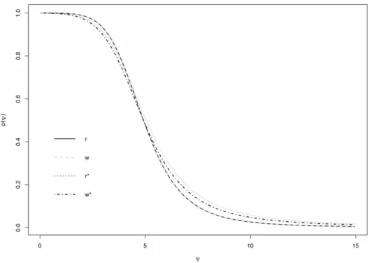
Let us consider a sample of five aggregate claims:
3.24, 4.39, 1.30, 11.51, 4.15.
Assume the Poisson-Exponential model and our aim is to obtain inference for the mean aggregate claims. Figure 1 plots thep-value functions obtained by the signed likelihood root method (r), the likelihood ratio method (w), the modified signed likelihood root method (r∗) and the simulated Bartlett corrected likelihood ratio method (w∗), respectively. From the plot, the signed likelihood root method and the likelihood ratio method give exactly the same result because former is the signed root of the later, and
they are different from the modified signed likelihood root method and the simulated Bartlett corrected likelihood ratio method.
Figure 1: The p-value function plot for four inference methods. r represents the signed likelihood root method,wrepresents the likelihood ratio statistic,r∗
represents the modified signed likelihood root method andw∗ represents the simulated Bartlett corrected likelihood ratio method. Note thatrandwcoincide with one another.
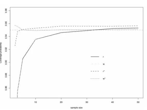
In order to compare the accuracy of the four methods, simulation studies are performed. Moreover, the coverage probability of the confidence interval is used as the criterion for determining whether a method is accurate or not. Furthermore, the coverage probability is used to examine how close the proportion of samples not being rejected atαlevel of significance is to the chosen nominal coverage level 1−α. Table
1 records the results and Figure 2 gives the visual idea of accuracy from a simulation with the following parameterization set-up:
1. Nis distributed as Poisson(λ=10).
2. X1, . . . ,XNare identical and independently distributed as exponential with mean
β=0.5, andS=X1+X2. . .+XN.
3. 5000 simulated samples ofSof sizenare generated, wheren=2,3,5,10,20,50. 4. To obtain ˆB, we useM=1000.
5. Report the proportion ofp(ψ=λ, β=5)>1−α=0.95 for each method discussed
in this paper.
It is clear that the simulated Bartlett corrected likelihood ratio method gives results closest to the nominal level 1−α = 0.95 even when the sample size,k, is as small as
2. It is followed closely by the modified signed lilelihood root method. The other two methods, the likelihood ratio method and the signed likelihood root method, do not give satisfactory results, especially when the sample size is small.
Table 1: The coverage probability of the 95% confidence interval at different sample size
n r(ψ) w(ψ) r∗(ψ) w∗(ψ) 2 0.7660 0.7648 0.9258 0.9572 3 0.8558 0.8552 0.9480 0.9554 5 0.9056 0.9044 0.9510 0.9500 10 0.9356 0.9354 0.9528 0.9490 20 0.9460 0.9454 0.9560 0.9504 40 0.9524 0.9516 0.9558 0.9506 50 0.9532 0.9528 0.9566 0.9512
A visual comparison of the accuracy level of the simulation result is presented in Figure 2. We observed that, as sample size increases, all the results are converging to the nominal value. However, when the sample size is small, the simulated Bartlett corrected likelihood method is extremely accurate with the modified signed likelihood root method closely following. This observation supports the theory that the former has fourth-order accuracy,O(n−2
), whereas the latter has third order of accuracy,O(n−3/2
). Moreover, the other two methods have only first-order accuracy,O(n−1/2). Furthermore, the simulated Bartlett corrected likelihood method can easily be implemented into standard statistical software, such asR.
Figure 2: Coverage probability plot of 95% confidence interval. The horizontal dash line is the 95% nominal level. rrepresents the signed likelihood root method,wrepresents the likelihood ratio method,r∗represents the modified signed likelihood root method andw∗
represents the simulated Bartlett corrected likelihood ratio method. Note thatr andwcoincide with one another.
In Appendix B, we reported results from a sample of other simulation studies with different choices of parameter values that we have performed. The results are similar to what we have presented here. More simulation studies have been carried out and the results are available upon request from authors.
6
Conclusion and Discussion
In this paper, two methods are proposed to obtain inference for the mean of the Poisson-Exponential distribution. One is based on the modified signed likelihood root method, where all equations are derived. The other method is an algorithm we developed to
approximate the Bartlett corrected likelihood ratio method. From the simulations we conducted, we observed that the simulated Bartlett corrected likelihood ratio method is extremely accurate even when the sample size is extremely small. A drawback of the modified signed likelihood root method is the complication in deriving the required statistics. Theoretically, the Bartlett corrected likelihood ratio method has an order of accuracy O(n−2), while the modified signed likelihood root method has an order of accuracy O(n−3/2) only. Our study confirms that the approximated Bartlett corrected likelihood ratio method proposed does achieve a better accuracy level than the modified signed likelihood ratio method in this case. Another advantage of the Bartlett corrected likelihood ratio method is that it can be applied to a vector parameter of interest, whereas, the modified signed likelihood ratio method is restricted to the scalar parameter of interest.
Appendix
Appendix A
Derivation of equations (12) and (13).
The density function of S is approximated by the saddlepoint approximation method and is presented in (1). Since ˆtin (3), we have
1−βtˆ=1−β1 β 1 − λβ s !1/2
= λβ s !1/2
Substituting ˆt,K(2)S (ˆt) andKS(t) into (1) we have
fS(s) = c q
K(2)S (ˆt)
expnKS(ˆt)−tsˆ o
= q c
2λβ2
(1−βt)3
exp λ " 1 1−βt −1
# −1 β 1 − λβ s !1/2
s
= p c
2λβ2(λβ/s)−3/2 exp
λ λβ s !−1/2
−1 − s β 1 − λβ s !1/2
= r c
2s−1 √
λβ
λ√s
exp
λ λβs
!1/2
−λ− s
β +
λ√s
p λβ
= √c
2s−1
p λβ
λ√s
−1/2
exp
2λ s
λβ
!1/2
−λ− s
β . Thus
`(λ, β;si) = loga+logfS(si)=log c q
2s−i1 p λβ
λ√si
−1/2
exp
2λ si
λβ
!1/2
−λ−si
β =
loga+log q c 2s−i3/2
−1
4log(λβ)+ 1
2logλ+2
√
si pλ
λβ−λ−si/β,
As explained in Section 3, without loss of generality, those terms that do not depend on parameters are set to 1 because they will not affect the rest of the likelihood-based calculations. Therefore, the log-likelihood function for a random sample (s1,s2, . . . ,sm) is
`(λ, β;s1,s2, . . . ,sm) =
m X
i=1
`(λ, β;si)
=
m X
i=1
−1
4log(λβ)+ 1
2logλ+2
√
si pλ
λβ−λ−si/β
= −m
4 log(λβ)+ m
2 logλ+2( m X
i=1
√
si)pλ
λβ−mλ−
Pm
i=1si
β .
which gives (12). With the reparameterizationψ=λβ, we have
`(λ, ψ;s1,s2, . . . ,sm) = −
m
4 log(ψ)+ m
2 logλ+2( m X
i=1
√
si)pλ
ψ −mλ−
m X
i=1 siψλ
which gives (13).
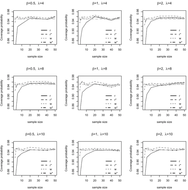
Appendix B
Results of simulation studies from different choices ofβandλ. The set-up of these studies is the same as the one presented in Section 5, but with differentβandλvalues. As observed from these plots, the simulated Bartlett corrected likelihood ratio method is extremely accurate with the modified signed likelihood root method closely following. The other two methods do not give satisfying results especially when the sample size is small.
Other simulation results are available upon request.
10 20 30 40 50
0.86
0.90
0.94
0.98
β=0.5, λ=4
sample size C ove ra ge p ro ba bi lit y r r* w w*
10 20 30 40 50
0.86
0.90
0.94
0.98
β=1, λ=4
sample size C ove ra ge p ro ba bi lit y r r* w w*
10 20 30 40 50
0.86
0.90
0.94
0.98
β=2, λ=4
sample size C ove ra ge p ro ba bi lit y r r* w w*
10 20 30 40 50
0.86
0.90
0.94
0.98
β=0.5, λ=8
sample size C ove ra ge p ro ba bi lit y r r* w w*
10 20 30 40 50
0.86
0.90
0.94
0.98
β=1, λ=8
sample size C ove ra ge p ro ba bi lit y r r* w w*
10 20 30 40 50
0.86
0.90
0.94
0.98
β=2, λ=8
sample size C ove ra ge p ro ba bi lit y r r* w w*
10 20 30 40 50
0.86
0.90
0.94
0.98
β=0.5, λ=10
sample size C ove ra ge p ro ba bi lit y r r* w w*
10 20 30 40 50
0.86
0.90
0.94
0.98
β=1, λ=10
sample size C ove ra ge p ro ba bi lit y r r* w w*
10 20 30 40 50
0.86
0.90
0.94
0.98
β=2, λ=10
sample size C ove ra ge p ro ba bi lit y r r* w w*
Figure 3: Coverage probability plot of 95% confidence interval. The horizontal dash line is the 95% nominal level. rrepresents the signed likelihood root method,wrepresents the likelihood ratio method,r represents the modified signed likelihood root method andw represents the simulated Bartlett corrected likelihood ratio method. Note that visuallyrandwcoincide with one another.
References
Alya, A. M., and Low, H. C. (2013), Saddlepoint approximation to cumulative distribution function for poisson-exponential distribution. Modern Applied Science,
7, 26-32.
Barbour, A. D., and Chryssaphinou, O. (2001), Compound poisson approximation: A user’s guide.The Annals of Applied Probability,11, 964–1002.
Barbour, A. D., Johnson, O., Kontoyiannis, I., and Madiman, M. (2010), Compound poisson approximation via information functionals.Electron. J. Prob.,15, 1344–1369. Barndorff-Nielsen, O. E. (1986), Inference on full and partial parameters based on the
standardized signed log likelihood ratio.Biometrika,73, 307–322.
Barndorff-Nielsen, O. E. (1991), Modified signed log likelihood ratio. Biometrika, 78, 557–564.
Bartlett, M. S. (1937), Properties of sufficiency and statistical tests. Proceedings of the Royal Society of London,160, 268–282.
Bero, R. (2003), Ckerstan’s method for compound poisson approximation.The Annals of Probability,32,1754–1771.
Daniels, H. E. (1954), Saddlepoint approximations in statistics.Annals of Mathematical Statistics,25, 631–650.
Daniels, H. E. (1987), Tail probability approximations. International Statistical Review,
55, 37–48.
Fraser, D. A. S. (2017), p-values: The insight to modern statistical inference. Annual Review of Statistics and Its Application,4, 1–14.
Fraser, D. A. S., and Reid, N. (1995), Ancillaries and third-order significance. Utilitas Mathematica,7, 33–53.
Fraser, D. A. S., Reid, N., and Wu, J. (1999), A simple general formula for tail probabilities for frequentist and bayesian inference.Biometrika,86, 249–264.
Ghribi, A. and Masmoudi, A. (2013), Acompound poisson model for learning discrete bayesian networks.Acta Mathematica Scientia,33, 1767–1784.
Kalbfleisch, J. G. (1985),Probability and Statistical Inference Volumne 2: Statistical Inference (2nd Edition). Springer-Verlag, New York.
Lugannani, R., and Rice, S. (1980), Saddlepoint approximation for the distribution of sums of random variables.Advances in Applied Probability,12, 475–490.
Murphy, S. A., and Van der Vaart, A. M. (2000), On profile likelihood.Journal of the American Statistical Association,95, 449–465.
Reid, N. (2010), Likelihood inference. Wiley Interdisciplinary Reviews: Computational Statistics,2(5), 517–525.
Thmazella , V. L. D., Cancho, V. G., and Louzada V. (2013), Bayesian reference analysis for the poisson-exponential lifetime distribution.Chilean Journal of Statistics,4, 99–113.