Computational Simulation of Marangoni
Convection Under Microgravity Condition
M.H. Saidi
1;, M. Taeibi-Rahni
1;2, B. Asadi
1and G. Ahmadi
3Abstract. In this work, the rising of a single bubble in a quiescent liquid under microgravity condition was simulated. In addition to general studies of microgravity eects, the initiation of hydrodynamic convection, solely due to the variations of interface curvature (surface tension force) and thus the generation of shearing forces at the interfaces, was also studied. Then, the variation of surface tension due to the temperature gradient (Marangoni convection), which can initiate the onset of convection even in the absence of buoyancy, was studied. The related unsteady incompressible full Navier-Stokes equations were solved using a nite dierence method with a structured staggered grid. The interface was tracked explicitly by connected marker points via a hybrid front capturing and tracking method. A one eld approximation was used where one set of governing equations is only solved in the entire domain and dierent phases are treated as one uid with variable physical properties, while the interfacial eects are accounted for by adding appropriate source terms to the governing equations. Also, a Multi-grid technique, in the context of the projection method, improved convergences and computational stiness. The results show that the bubble moves in a straight path under microgravity condition, compared to the zigzag motion of bubbles in the presence of gravity. Also, in the absence of gravity, the variation of surface tension force due to interface curvature or temperature gradient can still cause the upward motion of the bubble. This phenomenon was explicitly shown in the results of this paper.
Keywords: Marangoni convection; Microgravity condition; Hybrid front capturing and tracking method; Rising bubble; Multi-grid method.
INTRODUCTION
The variation of surface tension due to temperature gradient can initiate the onset of convection which is known as the common Marangoni convection. Note that, in the absence of temperature gradient, a variable surface tension force (not surface tension coecient) may be generated due to the presence of surface curvature gradient. The variation of surface tension force can lead to a convective motion which is referred to as hydrodynamic convection.
The Marangoni convection is particularly
impor-1. Center of Excellence in Energy Conversion, School of Mechanical Engineering, Sharif University of Technology, Tehran, P.O. Box 11155-9567, Iran.
2. Department of Aerospace Engineering, Sharif University of Technology, Tehran, P.O. Box 11155-9567, Iran.
3. Department of Mechanical and Aeronautical Engineering, Clarkson University, Potsdam, P.O. Box 13699-5725, NY, USA.
*. Corresponding author. E-mail: saman@sharif.edu
Received 3 November 2008; received in revised form 3 March 2009; accepted 19 May 2009
tant in the absence of buoyancy. It plays a crucial role in many applications, such as in crystal growth under microgravity condition, which is of interest to microelectronic industries. Understanding the thermo-capillary processes, especially the process of initiation of convection and when the ow become irregular, is very important for the corresponding manufacturing processes. Most earlier technological or scientic work performed under microgravity conditions was con-cerned with the improvement of the material processing procedures, while the fundamental uid mechanics of the process is not fully understood. Another important application is the boiling heat transfer for enhancing the heat exchange processes under microgravity con-ditions. Again, the fundamentals of the micrograv-ity boiling process are not fully understood. It is, therefore, important to have a thorough understanding of the process of bubble formation and motion under low gravity conditions where buoyant rise is negligible. Otherwise, understanding the physics of bubble motion under microgravity conditions is of great interest to a number of human life support applications in space.
In this work, the isothermal rising of a single bubble in a quiescent liquid under microgravity con-ditions was computationally investigated. The path of the bubble and the corresponding hydrodynamic Marangoni convection were evaluated. Note that the bubble was limited to a two-dimensional shape which is a severe approximation employed to allow reasonable resolution and computational requirements. However, such a formulation allows us to observe the sole eect of the bubble dynamics. In addition, the non-isothermal rising of a bubble was selected and Marangoni convection was studied in this paper.
For numerical simulation of the dynamics of large bubbles, the capturing and tracking of the interface is the most critical component. The computational results of Tryggvason et al. [1] have shown that the most accurate method for simulation of such ows is the hybrid front capturing and tracking technique. Although the eorts to compute multiphase ows are as old as Computational Fluid Dynamics (CFD), solving the full Navier-Stokes equations in the presence of a deforming interface has proven to be quite challenging. Only in recent years, major progress has been achieved with the use of the hybrid front capturing and front tracking method and also the level set method.
In addition to the hybrid front capturing and front tracking technique, several other techniques have been used in the past. A summary of the relevant techniques is provided here:
1. The oldest and still the most popular approach is to capture the interface directly on a regular and stationary grid. The MAC method in which marker particles are advected for each uid particle, and the VOF method where a marker function is advected are the best known examples. In the earlier implementations of these techniques, the stress condition at the interfaces was satised rather crudely. However, a number of recent developments including a technique to include surface tension [2] and the use of \level sets" [3] to mark the uid inter-face, has increased the accuracy of these techniques and thus their applicability.
2. The second class which potentially oers the highest accuracy uses separate boundary tted grids for each phase. The steady rise of buoyant, deformable and axisymmetric bubbles was simulated by Ryskin and Leal [4] using this method. Using this ap-proach, Dandy and Leal [5] also examined the steady motion of deformable axisymmetric droplets, while Kang and Leal [6] extended this methodology to axisymmetric unsteady bubble motion. The work of Leal et al. [4-6] had a major impact on subsequent research work in this area.
3. The third class is Lagrangian methods where the grid follows the uid. Recent examples include
two-dimensional computations of the break up of a droplet by Oran and Boris [7].
4. The fourth category is the front tracking method where a separate front marks the interface, but a xed grid which is only modied near the front is used for the uid within each phase. This technique has been extensively developed by Glimm [8].
As mentioned earlier, in this work we used the hybrid front capturing and front tracking method of Tryggvason et al. [1] which is a combination of front capturing and front tracking techniques. In this method, a stationary regular grid is used for the uid ow, while the interface is tracked by a separate grid (front grid) that is embedded on the rst one but moves with the interface. Note that, in the hybrid front capturing and front tracking method, all phases are treated by a single set of governing equations, while in the front tracking method, each phase is treated separately. This method was developed by Unverdi and Tryggvason [1,9]. Loth et al. [10-12] used this method to investigate the shear ow modulation and bubble dispersion of a bubbly mixing layer ow. Others also used this method to examine a number of other multiphase ow problems, e.g. the collision of two equal size droplets [13]. Another use of this method was the study of the breakup of accelerated droplets where both \bag" and \shear" breakup have been observed [14].
Multiphase ow computations involve coupled momentum, mass and energy transfer between mov-ing and irregularly shaped boundaries, large property jumps between materials and computational stiness. In this study, we focus on a combined Eulerian-Lagrangian method to investigate performance im-provement using the multi-grid technique in the con-text of the projection method. The main emphasis was on the interplay between the multi-grid computation and the eect of the density ratios between phases. As the density ratio increases, the single grid computation becomes substantially more time-consuming; with the present problems, an increase of factor 10 in density ratio results in, approximately, a three-fold increase in CPU time. Overall, the multi-grid technique speeds up the computation and, furthermore, the impact of the density ratio on the CPU time required was substantially reduced [15-17].
IMPORTANT DIMENSIONLESS NUMBERS The rise of a bubble in a quiescent liquid and its associated convection depend on the liquid physical properties, such as density, kinematic viscosity and surface tension. The most important physical dimen-sionless numbers in such a ow are: bubble Reynolds number, ReB, Bond (Eotvos) number, Eo (Bo), Morton
number, Mo, Weber number, We, Marangoni number, Ma, and Froude number, Fr, dened, respectively, as:
ReB= 2UTreq; (1)
Eo (Bo) = 4r2eqg; (2)
Mo = g433; (3)
We =2UT2req
; (4)
Ma = @T@@T@xL2; (5)
Fr = UT2
2greq: (6)
Here, req = 3V41=3 and and are the density
and the kinematic viscosity of the liquid, respectively. Note that the Morton number is related to the liquid physical properties and is independent of the ow conditions. Liquids can be categorized in dierent groups, namely those with high Morton numbers (Mo > 10 2), those with intermediate Morton numbers and
those with low Morton numbers (Mo < 10 6). On
the other hand, the Bond number characterizes the bubble size so that a functional relationship between any parameter and the Bond number describes how that parameter changes with the bubble volume. The terminal rise velocity of bubble (UT) in Denition 1 is
a function of equivalent radius, density, kinematic vis-cosity, gravitational acceleration and surface tension. Note that, in most practical applications, interest is mainly in low Morton numbers and moderate Reynolds numbers (between 200 and 900). At lower Reynolds numbers, however, bubbles have an approximately spherical shape, and they rise in a rectilinear path.
Whereas, at intermediate and high Reynolds numbers, bubbles become oblate ellipsoids and rise in an irregular (zigzagging or spiraling) fashion. The summary of observed path and transition criteria at normal gravity is listed in Table 1 [18].
A ow induced by surface tension gradients or thermal gradients is termed Marangoni convection. For most uids, the temperature gradient of surface tension
@ @T
is negative and regions of higher temperature ex-hibit a reduced surface tension. Therefore, Marangoni convection, according to a Ma Number, results in a recirculating uid ow from the warmer to the colder regions of a liquid and small temperature gradients give rise to relatively high uid velocities along the phase boundary [19].
GOVERNING EQUATIONS
As noted before, in the hybrid front capturing and front tracking technique used here, only one set of governing equations is used for both phases, which requires accounting for the interfacial eects by adding the appropriate source terms to the governing equa-tions [20,21]. Since the physical properties and the ow eld are discontinuous across the interface, all variables must be interpreted in terms of generalized functions. Thus, various uids can be identied by a step (Heaviside) function (H) which takes the value of one-for-one particular uid and zero for the other. The interface is marked by a non-zero value of the gradient of the step function. It is most convenient to express H in terms of an integral over the product of one-dimensional -functions as follows:
H(x; y; t) = Z
A
(x xf)(y yf)dA: (7)
The density as well as any other physical properties can be written in terms of both the constant densities on either side of the interface and the above Heaviside
Table 1. Summary of some previous experimental results about bubble shape under normal gravity [18]. Observed Shapes and Onset of Shape Instability
Spherical Ellipsoidal Unstable Aybers & Tapucu (1969) req< 0:42 mm req< 1:00 mm req> 1:00 mm
We > 3:7 Haberman & Morton (1954) Re < 400 400 < Re < 5000
Miksis et al. (1981) We > 3:23 Ryskin & Leal (1984) Contaminated liquids Re > 200
Pure liquids We > 3 4 Duineveld (1994,1995) We > 4:2
req> 1:34 mm
function as:
(x; y; t) = iH(x; y; t) + o(1 H(x; y; t)): (8)
Here, i and o are the density at H = 1 and 0,
respectively. On the other hand, for the viscous term, the full deformation rate tensor is implemented, while the conservative form of the advection term is normally used. Thus, the linear momentum equation is written as:
D(u)
Dt = rP + g + r:(ru + rTu)
+ kn(x xf): (9)
Note that the surface tension forces have been added as a delta function which is non-zero only on the bubble surface where x = xf. The interface force acting on
the marker points is spread to the nearby grid points using the discrete Delta function dened as follows:
(x xk)
= 8 < :
0; otherwise
3
Q
n=1 1 dp
1 + cos(x xdpf); if x xfd p (10)
The mass conservation law is written as: @
@t + r:u = 0: (11)
In this work, the ows of uids are both assumed to be incompressible so that the density of a uid particle in the ow eld remains constant. Thus:
D
Dt = 0; (12)
and:
r:u = 0: (13)
The viscosity of each uid particle is also assumed to be constant. Thus:
D
Dt = 0: (14)
The thermal energy equation with an interfacial source term to account for the liberation or absorption of latent heat is:
D(cpT )
Dt = r:k0(rT ) + _mfL(x xf);
L = L0+ (c1 c2)Tsat: (15)
Here, T is the temperature and L0 is the latent heat
measured at the equilibrium saturation, Tsat(P ),
corre-sponding to the reference ambient system pressure [22].
NUMERICAL METHODOLOGY
In this work, the unsteady Navier-Stokes equations are solved using the nite dierence method with a staggered xed structured grid, while the interface (front) is tracked explicitly by connected marker points. The interfacial source term (surface tension eect) is computed at the front grid points and is interpolated on the xed grid. The advection of uid properties, such as density is accounted for by following the motion of the front. Figure 1 shows the xed Eulerian and the moving Lagrangian grids used.
For solving the governing equations, the following points have to be accounted for:
The density and the viscosity changes due to the phase transport.
The surface tension eect is only at the front. Accurate evaluation of velocity and the pressure
elds at each time step.
Accurate evaluation of the motion of the interface itself.
Figure 1. Eulerian and Lagrangian grids in hybrid front capturing and front tracking technique.
The procedure used for evaluation of the density and viscosity transport and the surface tension term is the key element in the numerical approach. In the Volume Of Fluid (VOF) approach, an indicator func-tion is used to identify dierent phases of the ow. In the hybrid front capturing and front tracking approach, however, the interface is explicitly marked and tracked. Knowing the location of the front, the values of the uid property at dierent ow locations are easily specied. However, identication of the moving front is associated with the following diculties:
How to best identify the front;
How the data are transported between the xed and moving grids;
How the front moves with time;
How to satisfy the conservation laws as the front shape changes during its motion.
In the present approach, as the front shape changes, some grid points are added or subtracted to maintain a proper grid for the front. Figure 2 shows a typical restructuring of the front grid. In the hybrid front capturing and front tracking approach when data is transferred between the two grids, it is very important that the conservation laws are satised. To advect the discontinuous density and viscosity elds, and to compute surface tension forces, the bubble surface is represented by separate computational el-ements, referred to as the front. The front grid is of one lower dimension than the stationary uid grid and is advected by the uid velocity which is interpolated from the uid grid. To inject surface tension forces onto the xed uid grid, a technique that is usually called the Immersed Boundary Method and which was introduced by Peskin, is used. In this approach, the innitely thin interface is approximated by a smooth distribution function which is used to distribute the surface forces over the grid points close to the surface in such a way that the total forces are conserved. Therefore, the front is given a nite thickness of about three to four grid spacings and there is no numerical diusion of this front, since the thickness remains constant for all time. To generate the density and viscosity elds from the front, a technique introduced by Unverdi and Tryggvason [9] is used which is based on distributing the jump in
Figure 2. Restructuring of a Lagrangian grid.
these quantities onto the xed grid by the Peskin technique and then solving a Laplace equation for the eld variable itself.
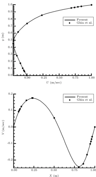
For code verication purposes, the incompressible lid-driven cavity ow was simulated. Figure 3 shows the X-velocity component prole along the vertical centerline and the Y -velocity component prole along the horizontal for Re = 100, which, in comparison with the results of Ghia et al. [23], show very good agreement.
For a bubble under micro-gravity conditions, grid independency studies were also performed for 98 66, 146 98, and 194 130 grids. The related results are summarized in Figure 4. It is seen that, for the st course grid, the shape of the bubble is distorted, but for the last two rened grids, the front shapes are roughly the same. Thus, the 146 98 grid was chosen for the sake of economy of the computations.
Figure 3. X- and Y - velocity components proles at the centerline of the cavity.
Figure 4. Grid independency study (case 2).
For a non-isothermal condition test case, the uids consist of the same ideal gas held at a uniform temperature (Ti); the position of the membrane was
Ri and the total mass of the gas in the enclosure
was m. Fluid B was heated adjacent to the walls by heat ux (q) for time t0. The temporal evolution of
the membrane radius is presented in Figure 5. The nal state for this case is in good agreement with the exact theoretical solution. The transient behavior seems to evolve in three phases: First, the heated uid, B, expands, causing a compression of uid A and, thus, decreases the membrane radius. The pressure in uid A rises until it exceeds that in B, upon which the membrane begins to re-expand. Once the heating ceases and the temperature in the enclosure begins to homogenize, the pressure in uid B drops further, relative to that in uid A, and the membrane continues to expand until it reaches a steady nal value.
RESULTS AND DISCUSSIONS
In this work, the rising of a single bubble in a quiescent liquid under microgravity conditions was computa-tionally simulated. In addition to general studies of microgravity eects, the initiation of hydrodynamic convection, solely due to the variations of interface curvature (surface tension force) and thus the gen-eration of shearing forces at the interfaces, was also studied. Then, the variation of surface tension due to temperature (Marangoni convection) can initiate the onset of convection even in the absence of buoyancy studied. The results show that the bubble moves in a straight path under microgravity condition compared to the zigzag motion of bubbles in the presence of grav-ity. The related unsteady incompressible full Navier-Stokes equations were solved using a conventional nite dierence method with a structured staggered grid. Also, a Multigrid technique in the context of the projection method improved convergences and computational stiness. The interface was tracked explicitly by connected marker points via a hybrid front capturing and tracking method.
Multi-grid iteration combines classical iterative techniques, such as the Gauss-Seidel line or point relaxation with sub-grid renement procedures to yield a method superior to the iterative techniques alone. By iterating and transferring approximations and cor-rections at sub-grid levels, a good initial guess and rapid convergence at the ne grid level can be achieved. Multiphase ow computations involve several challeng-ing issues. For example, the momentum, mass and energy transfer between phases are coupled. When the interface moves, one needs to compute the domain shape and associated geometric information, such as curvature and normal and projected area/volume, as part of the solution which adds nonlinearity to the
problem and can create diculties in grid generation. Oftentimes, there are large property jumps across the interface, e.g. the density ratio between vapor and water under standard sea level conditions is around 1,000, which results in multiple time and length scales and computational stiness. To deal with these issues, numerous numerical techniques have been developed, each with its own merits and diculties. The present approach tracks the interface with the Lagrangian method using massless markers while the eld equa-tion computaequa-tions are carried out with the Eulerian method on xed Cartesian meshes. The pressure equation which is a diusion-type for low speed ows, exhibits slower convergence rates than the convective-diusive ones when employing iterative matrix solvers. Therefore, improvement on the solver of the Poisson equation can accelerate the overall performance of the method. The property jump between phases also alters the convergence behavior. In this study, the moving boundary separating two uids and the eect of the property ratios between phases was used. The multi-grid technique works on the principle that high wave number components decay faster than low wave number components. A component's wave number is considered high or low, depending on the grid size. This dependence is such that low wave number components on a ne mesh behave like high wave number compo-nents on a coarse mesh. Therefore, treating the various wave number components on dierent grids makes it possible to accelerate the convergence rate.
Figure 6 shows typical bubble shapes in time for dierent density ratios; 10, 100. The initial bubble starts to rise due to the eect of buoyancy in the cylinder, and it eventually deforms to a steady-state shape. Figure 7 shows the number of ne grid iterations required to reach a residual level of 10 6
Figure 6. Bubble shapes evolution for dierent density ratios 10 (left) and 100 (right).
Figure 7. Residual history for dierent levels.
at the very rst time step, which requires the largest number of iterations to converge among all time steps, since it starts to iterate from initial conditions; one level represents the iteration history for a single grid computation. As demonstrated, the convergence rate improves dramatically when the level of the multi-grid is increased.
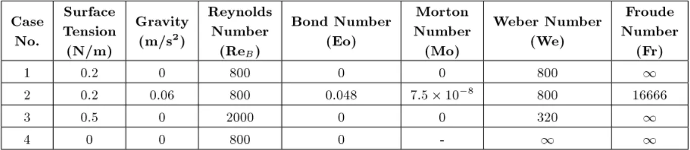
Dierent cases studied (for isothermal rising) are listed in Table 2. The selected simulation conditions are such that the bubble motion is under low or zero gravity. Dierent cases have been introduced in order to study both the buoyancy and hydrodynamic convection eects. According to Table 1, the bubble shape varies from spherical to ellipsoidal (or equivalent shape in 2 dimensions), for dierent Reynolds and Bond numbers. Also, depending on these shapes, the bubble follows a straight line or zigzag curve while moving upward.
The evolutions of the pressure and density elds are shown in Figure 8. The unsteady motion of the bubble is clearly shown in this gure.
Figure 6 shows the bubble shape evolution from circular at the initial stage to elliptical at later times, while following a straight path. Note that in cases 1, and 3, in the absence of gravity, the motion is only due to the curvature induced lift force given as:
Lift = kn(X Xf): (16)
This lift force is due to the surface tension coecient and interfacial curvature. However, for the initial cylindrical bubble, the value of this force is zero and, thus, its onset is due to an initial disturbance. It should be noted that a similar phenomenon, entitled \parasitic currents", has been reported especially for gas-liquid interfaces. Parasitic currents are unphysical currents generated in using implementations of the Continuum
Table 2. Dierent test cases considered in this study. Case
No.
Surface Tension (N/m)
Gravity (m/s2)
Reynolds Number
(ReB)
Bond Number (Eo)
Morton Number (Mo)
Weber Number (We)
Froude Number
(Fr)
1 0.2 0 800 0 0 800 1
2 0.2 0.06 800 0.048 7:5 10 8 800 16666
3 0.5 0 2000 0 0 320 1
4 0 0 800 0 - 1 1
Figure 8. Density (left) and pressure (right) shadowgraphs of bubble motion in a quiescent liquid under zero gravity condition (case 3).
Surface Force (CSF) technique to model surface tension forces in multi-phase computational uid dynamics problems. However, this phenomenon has a limited magnitude regarding uid properties [24]. Also, in our computational methodology, the CSF scheme has not been used. Then, it seems that some parts of this hydrodynamic convection can exist physically. Equation 16 shows that changes in the curvature or in the surface tension coecient can initiate bubble motion, even in the absence of gravity. Here, the surface tension coecient is constant (since there is no temperature gradient). Thus, the only driving force for the bubble motion is the variation in the shape of the interface and initial disturbance. Figure 9 shows the evolution of the shape of the bubble with time.
The results for case 2 are shown in Figure 10. As shown in this gure, when gravity is low, the buoyancy and the hydrodynamic forces tend to move the bubble. The resulting lift force is given as:
Lift = g + kn(X Xf): (17)
As expected from this gure, the bubble movement is faster here, compared to case 1.
Figure 11 shows the results related to case 3, where the surface tension coecient is higher, but still, gravity is set to zero. Note from this gure that the bubble has higher upward velocity in comparison with the results of case 1 where the surface tension coecient was lower. The driving force for the bubble motion in this case is the hydrodynamic convection eect caused by the changes in the bubble curvature. This force is larger than the driving force of case 1 due to a higher surface tension coecient.
Figure 12 shows the results of case 4 where both surface tension and gravity are zero. According to Equation 17, the lift force is zero and, thus, there is
Figure 9. Bubble evolution (case 1).
Figure 10. Bubble evolution (case 2).
Figure 11. Bubble evolution (case 3).
no bubble motion with time which is consistent with the results of Figure 12.
In Figure 13, cases 1, 3 and 4 are compared for t = 1 second. Note that in the absence of gravity, the higher the surface tension coecient is, the higher is the upward lift force that leads to a higher bubble velocity. Also, as shown in this gure, higher surface tension coecient causes a higher upward motion of the bubble.
The results of case 1, at longer times, are shown in Figure 14. The important point in this gure is that the bubble has a downward motion at t = 2 seconds. Here, the change in the direction of motion is due to the change in the sign of the lift force caused by changes in the bubble curvature (hydrodynamic convection eect).
Figure 13. The comparison of Marangoni force (cases 1, 2 and 4) at t = 1 sec.
Figure 14. Bubble evolution (case 1) showing negative lift at t = 2 second.
The evolutions of the temperature elds are shown in Figure 15 under zero gravity conditions. The unsteady motion of the bubble is clearly shown in this gure. Also, Isotherms (right) and Flow eld (left) for a bubble under micro gravity are shown in Figure 16. Another characteristic feature of Marangoni convection becomes obvious from the numerical simulation with an existing temperature gradient, i.e. this convection tends to reduce its driving temperature dierence. With the growing intensity of the Marangoni convec-tion, i.e. growing Marangoni number, the tempera-ture gradient along the interface is more and more reduced. As shown in Figures 15 and 16, the number
Figure 15. Temperature shadowgraphs of bubble motion in a quiescent liquid under zero gravity condition (initial temperature = 96, wall temperature = 110).
Figure 16. Isotherms (right) and ow eld (left) for a bubble under micro gravity.
of isotherms touching the bubble surface decreases with the increasing intensity of the ow. Even for the smallest temperature dierences along the bubble interface, i.e. small Marangoni numbers, a uid motion with a typical toroidal vortex can be observed. In contrast to buoyancy convection, no critical Marangoni number has to be reached for the onset of uid ow. With a growing Marangoni number, the isotherms are displaced from the bubble towards the rigid surfaces, leading to an increased heat transfer there.
CONCLUSIONS
In this work, large bubble motion in a quiescent liquid is computationally simulated by a hybrid front captur-ing and front trackcaptur-ing method. The main conclusions are as follows:
For all cases studied here (for the values of the dimensionless numbers studied), the bubble moves in a straight path, which is in contrast with the bubble motion under normal gravity conditions. At microgravity conditions, the driving force for the
bubble motion (isothermal) is the variation in the bubble surface curvature. Both the buoyancy and hydrodynamic convection eects create positive lift and thus tend to move the bubble upward. However, this trend continues up to the point where the lift force changes in direction and thus the bubble moves downward.
As the density ratio increases, the number of itera-tions required to reach the same residual level also increases. The multi-grid technique, in the context of the projection method, improved convergences and computational stiness.
With growing Marangoni number (for non-isothermal cases), the isotherm lines are displaced from the bubble towards the rigid surfaces, leading to an increased heat transfer there.
NOMENCLATURE
V bubble volume
g gravitational acceleration req equivalent radius
UT terminal velocity
u velocity vector eld surface tension coecient n normal unit vector at interface k interfacial curvature
P pressure
kinematic viscosity coecient Dirac delta function
H Heaviside function
xf; yf coordinates of nodes in moving grid
x; y coordinates of nodes in xed grid A the bubble surface area
T temperature
cp specic heat
c1 specic heat (primary phase)
c2 specic heat (secondary phase)
_mf interfacial mass transfer
k0 conductive coecient
L0 latent heat
REFERENCES
1. Unverdi, S.O. and Tryggvason, G. \Computations of multi-uid ows", Physica. D 60, pp. 70-83 (1992). 2. Brackbill, J.U., Kothe, D.B., and Zemach, C. \A
continuum method for modeling surface tension", J. Comput. Phys., 100, pp. 335-354 (1992).
3. Sussman, M., Smereka, P. and Osher, S. \A level set approach for computing solutions to incompressible two-phase ows", J. Comput. Phys., 114(1), pp. 146-159 (1994).
4. Ryskin, G. and Leal, L.G. \Numerical solution of free-boundary problems in uid mechanics. Part 2. Buoyancy-driven motion of a gas bubble through a quiescent liquid", J. Fluid Mech., 148, pp. 19-35 (1984a).
5. Dandy, D.S. and Leal, G.L. \Buoyancy-driven motion of a deformable drop through a quiescent liquid at intermediate Reynolds numbers", J. Fluid Mech., 208, pp. 161-192 (1989).
6. Kang, I.S. and Leal, L.G. \Numerical solution of axisymmetric, unsteady free-boundary problems at nite Reynolds number. I. Finite-dierence scheme and its applications to the deformation of a bubble in a uniaxial straining ow", Phys. Fluids, 30(7), pp. 1929-1940 (1987).
7. Oran, E.S. and Boris, J.P. \Numerical simulation of reactive ows", Elsevier, New York, 1st Ed. (1987). 8. Glimm, J. \Nonlinear and stochastic phenomena: The
grand challenge for partial dierential equations", SIAM Review, 33, pp. 625-643 (1991).
9. Unverdi, S.O. and Tryggvason, G. \A front-tracking method for viscous, incompressible multi-uid ows", J. of Comput. Phys., 100, pp. 25-37 (1992).
10. Loth, E., Taebi-Rahni, M. and Tryggvason, G. \De-formable bubbles in a free shear layer", Int. J. Multi-phase Flow, 23(5), pp. 977-1001 (1997).
11. Loth, E., and Taebi-Rahni, M. \Forces on a large cylindrical bubble in an unsteady rotational ow", AIChE Journal, 42(3), pp. 638-648 (1996).
12. Loth, E., Taebi-Rahni, M. and Tryggvason, G. \Flow modulation of a planar free shear layer with large bubbles-direct numerical simulations", Int. J. Multi-phase Flow, 20(6), pp. 1109-1128 (1994).
13. Nobari, M.R., Jan, Y.J. and Tryggvason, G. \Head-on collision of drops", Phys. Fluids, 8, pp. 29-42 (1996). 14. Han, J. \Numerical studies of drop motion in
ax-isymmetric geometry", PhD. Dissertation, Mech. Eng. Department, the University of Michigan, Ann Arbor, MI, USA (1998).
15. Adams, J. \Multigrid software for elliptic partial dierential equations: MUDPACK", NCAR Technical Note-357, pp. 51-72 (1991).
16. Press, W.H., Teukolsky, S.A., Vetterling, W.T. and Flannery, B.P., Numerical Recipes in Fortran, the Art of Scientic Computing, 2nd Ed., Cambridge University Press, London (1992).
17. Shyy, W., Francois, M., Udaykumar, H.S. and Tran-Son-Tay, R. \Moving boundary in micro-scale biouid dynamics", Applied Mechanics Reviews, 54, pp. 419-53 (2001).
18. Vries, A.W. \Path and wake of a rising bubble", PhD Dissertation, Mech. Eng. Department, Twent University, Netherlands (2001).
19. Han, Y.Y., Seiichi, K. and Yoshiaki, O. \Direct calculation of bubble growth, departure, and rise in nucleate pool boiling", Int. J. of Multiphase Flow, 27, pp. 277-298 (2001).
20. Peskin, C.S. and Fauci, L.J. \A computational model of aquatic animal locomotion", J. Computational Physics, 77, p. 85 (1988).
21. Esmaeeli, A. and Tryggvason G. \Direct numerical simulation of bubbly ows", J. Fluid Mech., 37, pp. 313-345 (2001).
22. Shin, S. and Juric, D. \Modeling three-dimensional multiphase ow using a level contour reconstruction method for front tracking without connectivity", J. of Computational Physics, 180, pp. 427-470 (2002). 23. Ghia, U., Ghia, K.N. and Shin, C.T. \High
Re-solutions for incompressible ow using the Navier-Stokes equations and a multigrid method", J. Comp. Physic, 48, pp. 387-411 (1982).
24. Harvie, D.J., Davidson, M.R. and Rudman, M. \An analysis of parasitic current generation in volume of uid simulations", J. Anziam, 46(E), pp. C133-C149 (2005).