c
Sharif University of Technology, February 2009
Generalized Curvilinear Coordinate Interface
Tracking in the Computational Domain
A.H. Nikseresht
1;, M.M. Alishahi
2and H. Emdad
2Abstract. Volume Of Fluid (VOF) is one of the most powerful methods to resolve free surface ows. In this study, a new algorithm is developed in a curvilinear coordinate system, which implements an implicit pressure based method (SIMPLE) with a staggered grid and a Lagrangian propagation of the interface, using the VOF method in the computational domain. Based on this algorithm, a computer code is generated and two test cases of dam-breaking problems, both in curvilinear and Cartesian grid systems, are examined and, then, two applications of this method, including ow through a curved gate under a dam and the impact problem of a circular cylinder, are presented. The results show good agreement with experimental and other computational results.
Keywords: Free-surface; Volume-of-uid; Front tracking; Curvilinear coordinate system; Dam-breaking
INTRODUCTION
Incompressible viscous ow with a moving free surface occurs in many instances, both in industry and in nature, such as environmental engineering, die-casting, injection molding processes, marine sciences and many others. The available numerical methods for solving such problems can be classied into moving and xed grid approaches. The moving grid approach is typically conned to special applications, due to limitations in the rezoning technique [1-3]. In this regard, the xed grid approach seems to be a more viable method whenever a general motion of free surface ow is considered [4].
Among the existing xed grid approaches, Harlow and Welch [5] proposed the well-known marker and cell method (MAC) that labels uid particles with markers. Nakayama and Mori [6] improved the MAC method to preclude the possibility of producing an unphysical liquid front advancement. In the MAC method, the region occupied by the uid is tracked by the location of the markers in the course of the uid motion. Such a method denes the uid region
1. Department of Mechanical Engineering, Shiraz University of Technology, P.O. Box 71555-313, Shiraz, Iran.
2. Department of Mechanical Engineering, Shiraz University, Shiraz, Iran.
*. Corresponding author. E-mail: [email protected]
Received 23 October 2006; received in revised form 4 August 2007; accepted 24 September 2007
rather than the free surface and, thus, requires large computer storage and additional computational time to move all the uid markers to new locations, especially when a three-dimensional problem is encountered [7]. Furthermore, a nite volume far from the free surface might be unrealistically overlled or partially lled with markers, due to numerical errors. Hirt and Nichols [8] introduced the Volume Of Fluid method (VOF) for incompressible ow with a moving free surface.
In the VOF method, the interface describes, im-plicitly, the data structure that represents the interface, which is the fraction, C, of each cell that is lled with a reference phase, say, phase 1. The scalar eld, C, is often referred to as the color function. The magnitude of C in the cells cut by the free surface is between 0 and 1(0 < C < 1) and, away from it, is either zero or one. The data, C, are given at the beginning of a computational cycle but no approximation of the interface position is known apriori. The method is implicit, since one needs to \invert" data C to nd the approximate interface position. In other words, an algorithm for interface reconstruction is needed. Typically, one can reconstruct the interface by the straightforward Simple Line Interface Calculation (SLIC) method [9], Flux Corrected Transport method (FCT) [10] or by various \Piecewise Linear Interface Calculation" (PLIC) methods [11,12]. The second and third methods give much better results than the rst method.
It should be mentioned that, in earlier studies, the VOF method was applied in the Cartesian coordinate. Some recent works that implement the VOF method in curvilinear coordinates are presented by Kothe et al., [13] who work mainly in the physical domain. Their methods have some diculties and cannot be easily used, along with operator split techniques.
In the present study, the nite volume method in the physical domain is used to solve the Navier-Stokes equations. However, the free surface equation is transferred to the computational domain and the free surface is resolved in that plane. The two steps of propagation and reconstruction are carried out in this domain. In the present work, the PLIC for the interface reconstruction method is used. The main advantages of the proposed technique, i.e. the PLIC-VOF method in the computational domain over the earlier method of PLIC, in the physical domain, are as follows: 1. Operator splitting in the computational domain is
more easily carried out than in the physical domain. In the computational domain, splitting can be done in each coordinate direction, separately.
2. The method of interface tracking (PLIC-VOF) in the computational domain needs less computer re-sources, because just one ux computation on each face is required compared to two-face computation in the curvilinear physical domain.
3. The extension of the PLIC method to 3-D in the computational domain is straightforward.
Incompressible Navier-Stokes equations are dis-cretized using the nite volume method, based on the Patankar pressure correction algorithm (SIMPLE) [14]. Hence, the appropriate numerical algorithm to solve the Navier Stokes equations, for a two-phase with a high-density dierence incompressible ow in the curvi-linear coordinate, is introduced. The performance of the proposed numerical procedure is examined through the solution of two well-documented dam-breaking examples in Cartesian and curvilinear coordinates and comparison of the results with the experiment is also presented.
GOVERNING EQUATIONS
A single set of governing equations, covering both liquid and the surrounding air, for incompressible ows, can be written in the following non-dimensionalized form [12]:
@u
@ + u @u @x+ v
@u @y
= @p@x+Rer2u; (1)
@v @+u @v @x+v @v @y
= @p@y 1
Fr2+
Rer2v; (2)
r:~u = 0; (3)
where L is an arbitrary characteristic length, Fr = pU1
gL
is the Froude no. and density and viscosity
are unity in the liquid region, which jump to another constant in the air region, i.e., =
1 in liquid
a
L in air
, = 1 in liquid
a
L in air
. This jump happens in a few cells across the interface, as explained in the following. At the interface, a kinematic, as well as a dynamic condition, should be applied. Note that the dynamic condition, i.e., continuity of pressure at the interface, is automatically implemented via solving N-S equations through the interface. The kinematic condition, which states that the interface is convected with the uid, can be expressed in terms of C, as follows:
@tC + u:rC = 0: (4)
and at any cells (denoted by ij) can be computed
using a simple volume average over the cell:
ij= CijL+ (1 Cij)a; (5)
ij = CijL+ (1 Cij)a: (6)
DISCRETIZATION OF EQUATIONS
The general transport equation for dependent variable is written as:
@()
@t + r:(u) r:( r) + B = 0; (7) where u; and are the velocity, density and diusion coecient, respectively and B is a source term, which generally depends on . Regarding the diusion term in Equation 7, in general, the curvilinear coordinate system will be decomposed into two parts. One part is similar to the discretized diusion term in an orthogonal curvilinear system and the other part contains mixed derivatives. Therefore, the numerical schemes that are mainly prepared for ux calculations in orthogonal coordinate systems, such as the QUICK or the Power-law scheme [14], can be equally applied in general curvilinear coordinates. The cross derivative terms are discretized with an alternative approximation that is introduced in [15].
Discretization of the Momentum Equations A staggered grid arrangement is adopted, in which the pressure computation at the geometric center of the control volume and the tangential velocity components, Ui, lie at the midpoints of the respective control
Ui = Si:u
jSij cos i; (8)
where Si are the surface area vectors and i are
the angles between the surface area vectors and the tangential vectors, ei. The unit tangent vectors, ei, are
calculated at the centers of the control volume surfaces and are locally parallel to the coordinate lines, i. In
order to discretize the momentum equations, auxiliary discretizations for the Cartesian velocity components are considered [16]. The resulting equation can be written as follows:
aPUP1=aEU0E1+aWU0W1+aNU0N1+aSU0S1+b0U1;
(9) where:
U01
E = a11uE+ a12vE; (10)
U01
W = a11uW + a12vW; (11)
U01
N = a11uN+ a12vN; (12)
U01
S = a11uS+ a12vS; (13)
b0
U1 = a11bu+ a12bv; (14)
with: a11=
S1
x
jS1j cos 1
P
; and:
a12= S 1 y
jS1j cos 1
!
P
:
In Equations 9 to 14, the primed velocities are recog-nized as the velocity components parallel to U1
P at the
neighboring points. It is seen that the primed velocity components, such as U01
E, are combinations of U1
and U2 and that a eld solution, in terms of these
velocities, cannot be obtained. This diculty can be easily removed by introducing the \actual" neighbors (e.g., U1
E) in the discretization equation as follows:
aPUP1 = aEUE1+ aWUW1+ aNUN1+ aSUS1+ b0U1
+ aE(U0E1 UE1) + aW(U0W1 UW2)
+ aN(U0N1 UN1) + aS(U0S1 US1): (15)
In Equation 15, terms such as aE(U0E1 UE1) and
similar terms in the source term, b0
U1, represent
the eect of curvature. They are equivalent to the discretized source terms, which would be resulted from tensor analysis. The discretized form of the momentum equations, with part of the pressure dierence term written explicitly, can be expressed as:
aPUP1 =
X
anbUnb1+ A1(Pw Pe) + bU1; (16)
aPUP2 =
X
anbUnb2+ A2(Ps Pn) + bU2; (17)
where nb denotes the neighbor, bU1 and bU2 include
all explicit terms and: Ai = a
i1
@y @2
+ ai2
@x @2
; (i = 1; 2): INTERFACE TRACKING
In the PLIC, at each time step, given the volume fraction of one of the two uids in each computational cell and an estimate of the normal vector to the interface, a planar surface is constructed within the cell having the same normal. This planar surface also divides the cell into two parts, each of which contains the proper volume of one of the two uids. This planar interface is then propagated by the ow, and the resulting volume uxes of each uid into neighboring cells are determined. The updated values of the volume fraction are found throughout the domain and the numerical simulation can proceed to the next time step. The next three subsections describe the procedure for estimating the normal vector, the construction of the interface in each cell and the propagation of the interface by the ow. It should be noted that all of these three steps are carried out in the computational domain, (1; 2). For this purpose, at rst, the volume
fraction equation: @C
@t + ~u rC = @C
@t + u @C @x + v
@C
@y = 0:0; (18) should be transformed to the computational domain as follows:
rC = Vol1
S1@C
@1 + S 2@C
@2
; (19)
where Vol is a volume of each cell. ~u rC = 1
Vol
~u S1@C
@1+ ~u S 2@C
@2
:
From Equation 8, we have ~uSi= UiSicosi then:
@C
@t + ~u rC = 0:0 ) @C
@t +
(U1S1cos
1)
Vol
@C @1
+(U2SVol2cos2)@@C
2 = 0:0: (20)
Now, if U = (U1jS1jcos 1)
Vol and V =
(U2jS2jcos 2)
Vol ,
then, Equation 20 has a similar form to its counterpart in the Cartesian coordinate:
@C @t + U
@C @1 + V
@C
Normal Estimation
Reconstruction is based on the idea that a normal vector, ~m, together with the fractional volume, C, determines a unique line interface cutting the cell. In the rst part of the reconstruction, a normal direction to the interface is estimated using a nite-dierence formula. The normal vector in the 1, 2 domain is
dened as:
~m = rC: (22)
At rst, a cell corner value of the normal vector, ~m, is computed at (i + 1=2, j + 1=2) by:
m1;i+1=2;j+1=2 =
1
2h(Ci+1;j Ci;j
+ Ci+1;j+1 Ci;j+1); (23)
m2;i+1=2;j+1=2 =
1
2h(Ci;j+1 Ci;j
+ Ci+1;j+1 Ci+1;j); (24)
where h = 1 = 2 = 1. Then, the required
cell centered values are computed from the cell corner values by averaging:
mij =14(mi+1=2;j 1=2+ mi 1=2;j 1=2
+ mi+1=2;j+1=2+ mi 1=2;j+1=2): (25)
Connecting Fractional Volume and Interface Position
In the second part of the reconstruction, an interface, which divides the computational cell into two parts containing the proper volume of each uid, must be found. This is achieved by deriving an explicit expres-sion, which relates the \cut" volume to parameter , which completely denes the interface. The problem can be stated as follows.
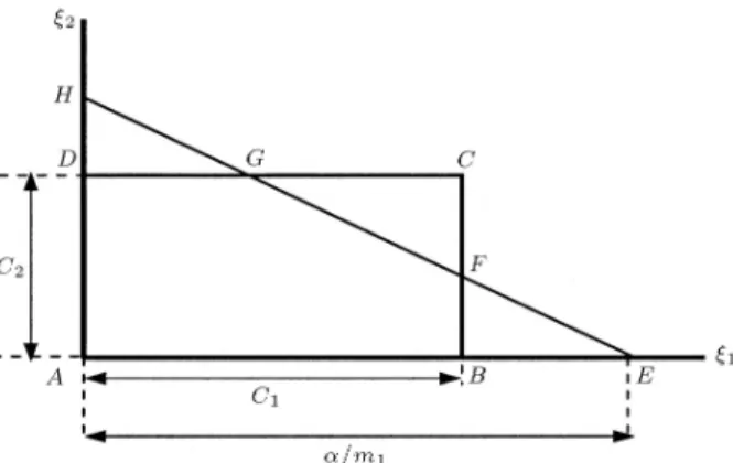
Given a rectangular (or square) cell of sides c1
and c2 in the (1, 2) plane, as depicted in Figure 1,
and a straight line (such as EH) with normal vector ~m, one must nd the area of the region (ABFGDA). To obtain an expression for this area, let one suppose that the components, m1 and m2, of the normal are both
positive. The most general equation for the straight line in the (1, 2) plane with normal ~m is:
m11+ m22= : (26)
This equation is similar to its Cartesian counterparts if (x1, x2) is substituted for (1, 2). Thus, the same
formulation for the area computation would be used in terms of (1, 2) [10,11].
Figure 1. The \cut area" refers to the region within the rectangle ABCD, which also lies below straight line EH, having normal m and parameter .
Lagrangian Propagation of the Interface Segments
Once the interface has been reconstructed, its motion, by the underlying ow eld, must be modeled by a suitable advection algorithm. This can be achieved by either an Eulerian or a Lagrangian scheme. The Lagrangian approach to the propagation of the inter-face can be best described by considering the way in which the given interface, Equation 26, is convected by the ow. For this purpose, rewrite Equation 26 with superscript (n) attached to all the variables,
m(n)1 1(n)+ m(n)2 (n)2 = (n); (27)
and think of this as the equation for the interface in a given cell at the initial time, tn. The Lagrangian
advection of this interface, by the ow, as time proceeds to tn+1 = tn + , will modify it to a new form,
which must be calculated. Since, in practice, the time stepping is performed separately in each spatial direction through operator splitting, the advection of the interface along any spatial coordinate, say 1, will
be described here.
To make the description simpler, let one suppose that the left face of the cell is located at 1 = 0, and
the right face at 1 = h = c1. Also, denote the 1
components of the velocity on the faces by U0and Uh,
as indicated in Formula 21. These are taken to be constant over the entire face to which they are assigned. The formulation in the general coordinate system will be the same as those of Cartesian coordinates [10-12] and only the x1 and x2 should be exchanged with 1
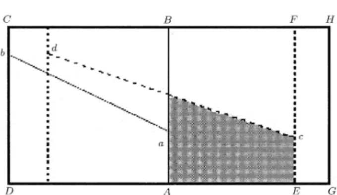
and 2. To illustrate the method, the procedure is
sketched in Figure 2. The shaded region represents the volume lost by the original cell and gained by the downwind cell, which can be calculated from parallel piped AEFB. With this procedure, the volume fraction eld is updated at time tn+1. This Lagrangian method
Figure 2. A schematic illustration of the Lagrangian propagation of the interface.
volume fraction, 0 C 1, when the CFL condition, (max juj)=h < 1=2, is satised. The programming of the Lagrangian method is considerably simplied by the fractional-step strategy, which can be easily applied in the computational domain.
NUMERICAL PROCEDURE The algorithm follows these steps:
a) Initialize the ow eld variables and, then, the numerical procedure in one time step is as follows. b) Propagate the volume fraction for the new time step, based on the velocity from the previous time step and update phase averaged quantities by the following sub steps:
1- Normal estimation;
2- Reconstructing the interface; 3- Propagating the interface;
4- Compute new values of C and other averaged quantities.
c) Use a SIMPLE algorithm to solve the ow eld governing equations.
d) Repeat b-c.
RESULTS AND DISCUSSION Dam-Breaking Flow
To examine the performance of the present numerical procedure, the results of two cases of dam-breaking problems are compared with the experimental and other numerical results. To show the robustness and versatility of the code, a random curvilinear grid, as well as a Cartesian grid, is used in the computation of the mentioned problems and results are compared with each other and experiments. Water and air are adopted as the media of the ow. The height and width of the water column of the two cases are (2.25 in, 2.25 in) and (4.5 in, 2.25 in). Corresponding Reynolds numbers, in terms of the height of the liquid region, are
43,129 and 121,986, respectively. In most free surface ows, the grid near the free surface should be ne, but in applications such as dam-breaking, since the ow sweeps through a great part of the domain at all possible inclinations, it is better to use ne grids in the entire ow eld. Thus, for simplicity, a uniform Cartesian grid and a random curvilinear grid system are used. For sure, a random general grid is not the proper choice for any uid ow problem. However, it provides a critical test case for the correctness and ro-bustness of the curvilinear coordinate algorithm when it produces the same results as those of a Cartesian grid. In the case of a (2.25 in, 2.25 in) problem, three grids, namely, 81 41, 101 51 and 201 101 grid points, are employed on the dimensionless domain of 0 x 4 and 0 y 2, which means Cartesian grid sizes of x = y = 0:05 and 0.04, respectively. The random curvilinear grid sizes of 101 51 for the rst case and 101 41 for the second case are presented in Figure 3. Also, the conditions applied on each boundary are depicted in Figure 3.
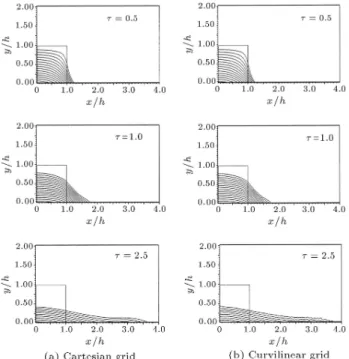
Figure 4 shows the resulting water front, xf(),
of the present study on various grids, for the case of a square water column, H = W = 2:25, in both grid systems. The results show no signicant dierence. The available experimental data [17] and the existing numerical results, such as the standard
Figure 3. Curvilinear grids of two cases of dam-breaking ows. (a) Case 1 with grids of (10151) and (b) Case 2
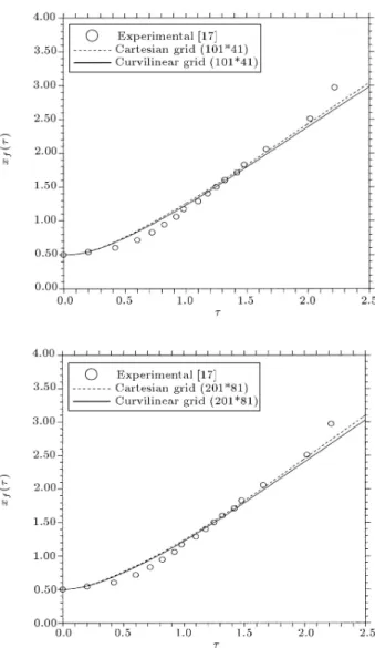
Figure 4. Comparison of waterfront xf() among the
present results with three grid systems and experimental data at various grid points for the case of (2.5 in * 2.5 in).
MAC method [5] and the modied MAC method [6] are also plotted in Figure 5. As shown in Figure 5, the MAC method overpredicts the experimental results, but the present work shows much better agreement with the experiment.
Considering that the Power-law scheme is of rst order accuracy, the discretization accuracy is also of the rst order. Therefore, the accuracy of the wave front computation in the present study is of order x. Figures 6 and 7 show the isobar and velocity vector of the rst case, (2.5 in * 2.5 in), at various
Figure 5. Comparison of waterfront xf() from the
present results, experimental data and other existing numerical results for the case of (2.5 in *2.5 in).
Figure 6. Isobars with increment of p = 0:05 at various times for the case of (2.5 in * 2.5 in).
Figure 7. Velocity vectors at various times for the case of (2.5 in * 2.5in).
time steps and compares the results of two systems of grid. The shape and position of isobars, including the waterfront, is almost the same in both grid systems. However, there are small wiggles in the right most regions of isobars, especially at later times. These might be due to an anomaly of randomly generated grids (Figure 3). It is obvious that the pressure is essentially near zero in the air region and this can be attributed to the negligible density of the air, as compared to the water. It is interesting to note, from velocity vectors in Figure 7, that the liquid motion induces a vortex in a layer of air adjacent to the free surface. This nding is consistent with physical reasoning.
In the second case of (4.25 in * 2.25 in), two grids, namely 101 41 and 201 81 grid points, are employed on the dimensionless domain of 0 x 10=3 and 0 y 4=3 in both Cartesian and curvilinear systems. Figure 8 presents a comparison of the present results of the Cartesian and curvilinear grids and shows good agreement between the results of these two grid systems. Figure 9 shows the comparison of a waterfront from dierent sources, including the results of the present work, the previous VOF code of Hirt and Nicholls [8] and the modied MAC method. It is obvious from Figure 9 that the Hirt and Nichols code [8] overpredicts the experimental data. The MAC results are more comparable with the experimental data in Figure 9 than with those of Figure 5, however, the
Figure 8. Comparison of waterfront xf() among the
present results with two grid systems and experimental data at various grid points for the case of (2.5 in * 2.5 in).
Figure 9. Comparison of waterfront xf() among the
present results and experimental data and other existing numerical results for the case of (4.5 in * 2.5 in).
consistency of the present results with experiments are almost the same in both cases.
Flow Under Sluice Gate
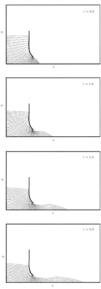
To present another example, which may be of some practical interest, consider a model of an arc gate with a dimensionless radius of 0.69, with the center at (1.67, 0.81), under a dam of the dimensionless height of 1.4, as shown in Figure 10. This gure shows the dimensionless geometry, dierent conditions on each boundary and the grid system. This example obviously shows the benets of using curvilinear grids and the simplications provided by the computational domain approach. Figure 11 presents the pressure distribution of the ow at various times. It can be seen that the free surface contracts around the exit, i.e. vena contracta, and at later times ( = 1:5, = 2:0), it re-expands as physically expected. In Figure 12, the velocity vectors of ow at various times are shown and it is obvious that, after the ow discharges with high velocity from the gate at some distance downstream, the uid velocity decreases and, thus, the elevation of the water front increases accordingly. It is interesting that the wiggles
Figure 10. Mesh system and dimensionless geometry of
Figure 12. velocity vectors at various times for ow out of opening gate.
in Figures 6 and 7 are absent in this case, indicating that these errors originate from the randomly generated grids in Figure 3.
Water Impact of Circular Cylinder
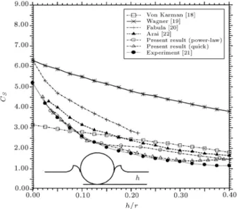
Another applicable example is the water impact of cir-cular cylinders, which has been studied extensively to clarify wave impact on members of oshore structures in a splash zone. The circular cylinder used in this calculation has a radius of 5.5 m. It is dropped with a constant velocity of 10 m/s. A grid system, with elements of (180 250) and the schemes of Power-Law and QUICK, were also used. In the present computational scheme, in order to avoid unsteady calculation and grid regeneration, a circular cylinder, as a rigid body, is xed to the grid system and, instead of moving the body downward, the free surface is forced to move upward. These conditions can be realized by imposing a continuous inow of the uid from the lower boundary of the physical domain and the moving side walls. The pressure on the upper boundary is also xed. The numerical results of this study, together with the published experimental, analytical and other numerical results, are shown in Figure 13. In this gure, the non-dimensional impact force, (f), namely the slamming coecient, (CS = 1=2Vf 2D), is
plotted as a function of the non-dimensional immersion height. As shown in this gure, the theoretical model of Von-Karman indicates an initial slamming coecient, CSo = [18], whereas that of Wagner and Fabula
gives CSo = 2 [19,20]. The experimental coecient,
CSo, exhibits a considerable degree of scatter, ranging
from 3.5 to 6.5 [21]. Based on experimental data, Campbell [21] proposed an empirical formula for the
Figure 13. Slamming coecients of circular cylinder (r = 5:5 m, V = 10 m/s) versus immersion height.
slamming coecient, as shown in this gure. The results of a nite dierence computation of Arai [22], also included in Figure 13, is based on inviscid ow. The present work results, of both Power-Law and QUICK schemes, are shown and the agreement with ex-perimental data is good, especially for QUICK schemes at h/r> 0:15.
With regard to the above examples, it can be expressed that the new method of PLIC-VOF interface tracking in the computational domain is robust and accurate enough to handle critical test cases, such as random grids, and produce acceptable results for applied and non-rectangular geometries.
CONCLUSION
A single set of dimensionless equations is derived to handle both liquid and air phases in viscous incom-pressible free surface ows. The momentum equations are solved using the SIMPLE method in a staggered grid. The Lagrangian approach in the computational domain is also applied in the context of a VOF method, to resolve the free surface eects. It is indicated that, with this new implementation of the PLIC-VOF method in the computational domain, it is an easy task to split the propagation algorithm, because the same algorithm as in the Cartesian grid is applied in the computational grid approach. The results of two cases of dam-breaking problems are presented, which show good agreement with experimental data and other numerical methods. The results for a random curvilinear grid and a Cartesian grid show the same agreement with experimental results. The application of a ow of water under a curved gate and a water impact problem, using curvilinear co-ordinates, are also presented. It can be concluded that the present method and the code are robust, produce results of good quality and, also, can be easily implemented.
REFERENCES
1. Frits, M.J. and Bories, J.P. \The Lagrangian solution of transient problems in hydrodynamics using a trian-gular mesh", J. Comput. Phys., 31, pp. 173-215 (1979). 2. Fyfe, D.E., Oran, E.S. and Fritts, M.J. \Surface tension and viscosity with Lagrangian hydrodynamics on triangular mesh", J. Comput. Phys., 76, pp. 349-384 (1988).
3. Lewis, R.W., Navti, S.E. and Taylor, C. \A mixed Lagrangian Eulerian approach to modeling uid ow during mould lling", Numer. Meth. Fluids, 25, pp. 931-952 (1997).
4. Chen, C.W., Li, C.R., Han, T.H., Shei, C.T., Hwang, W.S. and Houng, C.M. \Numerical simulation of lling pattern for an industrial die casting and its comparison
with the defects distribution of an actual casting", Trans. Am. Foundrymen's Soc., 104, pp. 139-146 (1994).
5. Harlow, F.H. and Welch, J.E. \Numerical calculation of time dependent viscous incompressible ow of uid with free surface", Phys. Fluids, 8, pp. 2182-2189 (1965).
6. Nakayama, T. and Mori, M. \An Eulerian nite ele-ment method for time dependent free surface problems in hydrodynamics", J. Numer. Meth. Fluids, 22, pp. 175-194 (1996).
7. Harlow, F.H., Amsden, A.A. and Nix, J.R. \Relativis-tic uid dynamics calculations with the par\Relativis-ticle-in-cell technique", J. Comput. Phys., 20, pp. 119-129 (1976). 8. Hirt, C.W. and Nicholls, B.D. \Volume of uid (VOF) method for dynamics of free boundaries", J. Comput. Phys., pp. 39-201 (1981).
9. Noh, W.F. and Woodward, P. \SLIC (Simple Line Interface Calculation)", Proceedings of the Fifth Inter-national Conference on Fluid Dynamics, A.I. Vande Vooren and P.J. Zandbergen, Eds., Lecture Notes in Physics, 59, Springer-Verlag, Berlin, p. 330 (1976). 10. Rudman, M. \Volume-tracking methods for interfacial
ow calculations", International Journal for Numeri-cal Methods in Fluids, 24, pp. 671-691 (1997). 11. Gueyer, D., Li, J., Nadim, A., Scardovelli, R. and
Zaleski, S. \Volume-of-uid interface tracking with smoothed surface stress methods for three-dimensional ows", Journal of Computational Physics, 152, pp. 423-456 (1999).
12. Nikseresht, A.H., Alishahi, M.M. and Emdad, H. \Volume-of-uid interface tracking with Lagrangian propagation for incompressible free surface ows", Journal of Science and Technology, 12(2), pp. 131-140 (Spring 2005).
13. Kothe, D.B., Rider, W.J., Mosso, S.I., Brock, J.S. and Hochstein, J.I. \Volume tracking of interface having surface tension in two and three dimensions", AIAA, 96-0859 (1996).
14. Patankar, S.V. \Numerical heat transfer and uid ow", Hemisphere, Washington, DC, USA (1980). 15. He, P. and Salcudean, M. \A numerical method for
3D viscous incompressible ows using non-orthogonal grids", International Journal For Numerical Methods in Fluids, 18, pp. 449-469 (1994).
16. Mousavi Mirkalaee, S.M. \Numerical study of two dimensional laminar incompressible ow around hov-ercraft", MSc Thesis, Department of Mechanical En-gineering, Shiraz University (Oct. 2001).
17. Martin, J.C. and Moyee, W.J. \An experimental study of the collapse of liquid columns on a rigid horizontal plane", Philos. Trans. Roy. Soc. London, 244A, pp. 312-324 (1952).
18. Von Karman, T., The Impact on Seaplane Float During Landing, NACA TN321 (1929).
19. Wagner, H., Landing of Seaplanes, NACA TM 622 (1931).
20. Fabula, A. \Ellipse tting approximation of two-dimensional normal symmetric impact of rigid bodies on water", Fifth Midwestern Conference on Fluid Mechanics, University of Michigan Press (1957). 21. Campbell, I.M.C. and Weynberg, P.A.
\Measure-ment of parameters aecting slamming", Wolfson Unit for Marine Technology and Industrial Aerodynamics, Univ. of Southampton, Report No. 440 (1980). 22. Makoto, A., Liang-Yee, C. and Yoshiyuki, I. \A
computing method for the analysis of water impact of arbitrary shaped bodies", Journal of The Society of Naval Architects of Japan, 176, pp. 233-240 (1994).