Solution of Three-Dimensional Line-of-Sight Guidance with a Moving Tracker

(1)

Solution of Three-Dimensional Line-of-Sight

Guidance with a Moving Tracker

S.H. Jalali-Naini

and V. Esfahanian 1

The closed-form solution of a three-dimensional line-of-sight guidance with a moving tracker is derived for an ideal case, in which a pursuer is always on the instantaneous line between the target tracker and the target. The solution can be applied to both surface-to-air and air-to-surface applications. Some signicant characteristics, such as intercept time, cumulative velocity increment, initial condition for interception, and the eect of acceleration limit, are also obtained and discussed. In addition, the equivalent eective navigation ratio for the line-of-sight guidance is introduced. Finally, solutions for a special case of maneuvering target are presented.

INTRODUCTION

In Line-Of-Sight (LOS) guidance, a pursuer maneuvers so as to be on the instantaneous LOS between the target tracker and the target. If the pursuer is always on the tracker-target LOS, then it will surely hit the target. This guidance law is also called 3-point guidance 1-9].

The dierential equation of the pursuer range, with respect to its angular position for LOS trajectory, is not integrable, even for a constant-speed pursuer and nonmaneuvering targets 4]. Locke gave a 10-term series solution for this problem 1]. The solution can also be described in terms of elliptic integrals 5]. Jalali-Naini and Esfahanian presented the closed-form solution of the LOS trajectory for nonmaneuvering targets, assuming the total pursuer acceleration to be equal to the required acceleration in the direction normal to the LOS 10,11]. This solution was extended to solve a modied LOS guidance 12]. A general dierential equation was then introduced by Shoucri to model the two-dimensional (2-D) trajectory of a pursuer for various guidance laws against maneuvering targets 13]. An approximate solution of the 3-D LOS guidance, for a pursuer with an arbitrarily time-varying velocity against maneuvering targets, was presented in 14], in which the pursuer commanded acceleration to be in the direction normal to the pursuer velocity. *. Corresponding Author, Aerospace Research Institute,

P.O. Box 15875-3885, Tehran 14666, I.R. Iran.

1. Department of Mechanical Engineering, University of Tehran, Tehran 14395, I.R. Iran.

In this study, the solution of the 3-D LOS trajec-tory for nonmaneuvering targets is derived for a moving tracker. Here, the total pursuer acceleration is also assumed to be equal to the required acceleration in the direction normal to the LOS. This solution is also valid for air-to-surface applications, whereas the previous solutions are only suitable for a stationary tracker. In addition, the analytical solution for a special case of maneuvering target is presented. Note that the minimum acceleration which must be applied in order to keep the pursuer on the LOS is termed \required acceleration".

EQUATIONS OF RELATIVE MOTION

The inertial OIxyz Cartesian coordinate system and the nonrotating Oxyz Cartesian coordinates with the origin xed at the moving target-tracker (point O), are shown in Figure 1. These two coordinate systems are coincident at ring instant. In the gure, M and T denote the pursuer and the target, respectively andrp

is the distance of particle P (pursuer M or target T) from the tracker, O. Consider the spherical coordinates (r") with origin at the target-tracker, in which

p =

A

p ;

A

(2)

": (1b)

The three relative acceleration components of particle P (arpapa"p) are as follows:

a_rp= rp;rp"_ 2

p;rp_ 2

pcos2"

p (2a)

a_p=rppcos"p+ 2_rp_pcos"p;2rp_p"_psin"p (2b)

a_"p=rp"p+ 2_rp"_p+rp_2

psin"pcos"p: (2c)

The preceding relations can be expressed in the form of:

r

p+

p(

p

r

p) (3b) where

p is the angular velocity vector of

r

p and is

given by:

p= (

r

p

v

p)=r 2

p (4a)

p=

q _

"2

p+ _2

pcos2"

p (4b)

It should be noted that Equations 3 are in terms of

p

instead of the angular velocity vector of the moving spherical coordinates!p =!rp

e

r+

p, in which !rp=

_

psin"p 12]. The reason is simple. Since:

_

!p

e

r=;!rp

+ _

p

e

r (5a) !p(!p

e

r) =!rp

+

p(

p

e

r) (5b) one has:

_

!p

e

r+!p(!p

e

r)= _

p

e

r+

p(

p

e

r): (6)

The angular momentum of unit mass for the relative motion (

H

p=

r

p

v

p) can be written as:

H

p= Hp

e

h=r2

p(;"_p

The other unit vector can be dened as

e

?

"): (8)

By the preceding denitions, Equations 3 can be expressed in the following form:

v

p= _rp

e

r+rpp

e

?

h (9a)

a

p= (rp;rp 2

?

h

e

h) constitutes new

moving coordinates, which are calledhcoordinates 15]. The relative acceleration vector can be expanded in this coordinate system with the components of (arpa?

pahp):

a

p=arp

e

r+a?

p

e

?

h +ahp

e

h: (10)

In terms of the h coordinates, Equations 2 can be rewritten as 16]:

rp;rp 2

p=arp (11a)

rp_p+ 2_rpp=a?

p (11b)

_

e

h=;

a_hp rpp

e

?

h: (11c)

Equations for a Nonmaneuvering Target and

Tracker

Consider a case in which the target and its tracker do not maneuver. In other words, their velocity vectors and the target relative velocity,

v

t, remain constant.

Therefore, the angle between the target relative ve-locity and the LOS, = cot;1

_

rt

t, decreases with time where the subscript \t" denotes the target (see Figure 1). In addition,h is dened to be the nearest distance from the tracker to the line along the target relative velocity vector.

The unit angular momentum for the target rel-ative motion remains constant for a nonmaneuvering target and tracker, that is:

Ht=rtvtsin=rt0vtsin

0 (12)

where the subscript \0" describes the initial value. Therefore:

rtsin=rt0sin 0=h

(3)

It can be seen thathis equal to H

t=vt. From Figure 1,

one can write: _

rt= vtcos (14a)

rtt= vtsin (14b)

where t is the tracker-target LOS rate. By

dier-entiating Equation 13 with respect to time and using Equation 14a, one obtains:

_

=;

vtsin2

h = ;

vtsin

rt (15)

Comparing Equations 14b and 15, one can conclude the relation t =;_. The other useful relations can then be found as:

= 2_2cot (16)

cot= cot0+ (vt=h

)t: (17)

The relations for (rtt"t) and their time derivatives

are simply derived in the moving Cartesian coordinates (xyz). For instance, one has:

r2

t =r2

t0+ 2(rt

0r_t0)t+ v 2

tt2 (18) tant=yt=xt= (yt0+ _yt0t)=(xt0 + _xt0t) (19) sin"t=zt=rt= zt0+ _zt0t

q

r2

t0+ 2rt

0r_t0t+ v 2

tt2

: (20) Using Equation 19 gives an expression for the current time as:

t= (xt0tant ;yt

0)=( _yt0 ;x_t

0tant) (21) and by substituting that into Equation 18 or 20, one can eliminate the current time,t, from the equations. Therefore, an explicit relation between rt and t or

"t and t can be obtained. Similar procedure can

be applied to obtain relations between the variables (_rt_t"_t) andt.

Assume that the target relative velocity is in the negativey direction and xt0zt0

6

= 0. One can obtain simple relations for this case as:

rt= (rt0sin"t0)=sin"t (22) tan"t= (tan"t0=cost0)cost (23) sin=(sin0=sin"t

0)sin"t= q

1;cos 2"

tsin2

t

(24) and for angular rates, one arrives at:

_

t=_t0 = cos 2

t=cos2

t0 (25) _

"t="_t0 = (sin 2"

tsint)=(sin2"

t0sint0): (26)

EQUATIONS OF LOS GUIDANCE

The basic guidance law in 3-point guidance ism(t) =

t(t) and "m(t) = "t(t), where the subscript \m",

denotes the pursuer. An ideal case is assumed, in which the pursuer is always on the line between the target tracker and the target without any error. If the pursuer is initially red at the target from the target tracker and maneuvers according to the following relations:

a_m=rmtcos"m+ 2_rm_tcos"m;2rm_t"_msin"m (27a)

a_"m=rm"t+ 2_rm"_t+rm_2

tsin"mcos"m (27b)

then, it will always remain on the tracker-target LOS. The proof of Equations 27 can be observed as follows. By the denitionm=rmcos"m, Equation 27a can be

rewritten asa_m=mt+ 2 _m_t therefore, one has:

m_dtd( _m;_t) + 2 _m( _m;_t) = 0: (28) The preceding relation is a linear rst-order dierential equation which has a solution in the form of2

m( _m; _

t) = constant. Thus, one has _m = _t. Using

Equation 27b, one can also obtain r2

m( _"m ;"_t) = constant. Hence, one has m(t) = t(t) and "m(t) =

"t(t). Hereafter, the subscript \m" or \t" will be

dropped forand"for convenience. It should be noted that a_rm = 0 is assumed. The value of a_rm does not cause any deviation from the LOS.

sin= v_vt_mrm_r_tsin (30)

where is the angle between the pursuer relative velocity and the LOS. By dierentiating Equation 29 with respect to time, one arrives at:

a

m

e

r= 2

v

t

v

m

mplos= 2(_rm

;

rm

rtr_t)

e

?

h +r_rm_t

a

tplos: (32) The pursuer relative acceleration can then be found as:

a

m=(rm;rm 2)

e

r+2(_rm;

rm

rtr_t)

e

?

(4)

or:

a

m= (rm;rm 2)

e

r+ (rm_ + 2_rm)

e

?

h +r_rm_taht

e

h:

NONMANEUVERING TARGET AND

TRACKER

Consider that the target and its tracker move with con-stant velocity vectors. The total pursuer acceleration is also assumed to be equal to the required acceleration in the direction normal to the LOS, therefore,a_rm= 0, which becomes:

rm;rm_

2= 0: (35)

By using: _

rm= _dr_dm (36)

rm= dr_dm+ _2d 2r

m

d2 (37)

and with the change of independent variabletto, one may rewrite the dierential Equation 35 in the form of

dr_dm+ _2

d2r

m

d2 ;rm

= 0: (38)

Using Equation 16, the preceding dierential equation simplies to :

d2r

m

d2 + 2cotdr

m

d ;rm= 0: (39) By changing the variableu=rmsin, one can rewrite

Equation 39 as: 1

sind

2u

d2 = 0 (40)

which has a solution in the following form:

rm= A1+A2

sin (41)

whereA1 andA2are integrating constants and can be determined from the initial conditions. From Figure 1, one may write:

_

rm= vmcos (42a)

rm = vmsin (42b)

In LOS guidance, the pursuer is initially red at the target from the tracker (rm0 = 0). By using Equations 42, one can conclude0= 0 and _rm

0 = vm0 therefore,

rm= nrt0( 0

;)

sin for 0

6

= 0 (43)

where n is the ratio of initial relative velocity of the pursuer to the target relative velocity (vm0=vt). By dierentiating Equation 43 with respect to time, one obtains:

_

rm= (vm0=sin

0)sin+ (0

;)cos] (44) One can also obtain the pursuer acceleration as:

am= 2vm0vt

hsin 0

sin3= 2h v

m0vtrt0

r3

t : (45)

Dividing Equation 42a by Equation 42b yields

rmcot=;drm=d therefore:

tan= 0

; 1 + (0

;)cot:

(46) By using the relation v2

m= _r2

m+r2

m2and after some manipulation, one derives:

v2

m= v

2

m0 sin2

0 (0

;)

2+ sin2+ ( 0

;)sin2]: (47) One may also write:

Vmsin =j

V

m

e

rj (48a)

Vmcos =

V

m:

e

r (48b)

in which , the pursuer velocity-to-beam angle, is the angle between the pursuer velocity vector and the LOS. Therefore:

tan = q

Vh2 O + (V

?

O +rm) 2 _

rm+VOr

(49)

where Vr

O, V ?

O and V

h

O are the components of the tracker velocity inhcoordinates.

The pursuer and target positions are equal at the collision instant, therefore, by equatingrmandrtfrom

Equations 13 and 43, one arrives at:

f =0

;(1=n)sin

0 (50)

where the subscript \f" denotes the nal value. Using Equation 17, intercepting time can then be found as:

tf = (h=v

t)(cotf;cot

(5)

Using Equations 13 and 43, for interception of the target, one must have:

n >sin0=0 for 0

6

= 0: (52)

The cumulative velocity increment is dened as: V =

Z t f 0

j

A

mjdt (53)

in which

A

mis the pursuer acceleration. Therefore, by

using Equation 45 and for a nonmaneuvering tracker (

A

m=

a

m), one arrives at:

V = (2vm0=sin

m= 2vm0vt

rt0sin 2"

0

(;cos

e

+ sin"sin

e

")sin 2"

(57) ;=sgn(xt0zt0)

sin;1

sin

c

;sin

;1

sin0

c

(58) where sgn() is the sign function andcis:

c=q

1 + cos2 0cot

2"

0: (59)

Equation 58 is valid forxt0zt0

6

= 0, but for xt0 = 0 orzt0 = 0, one has ; = 0. When xt0 = zt0 = 0 and

yt0 >0, the target will be intercepted before it passes through the tracker.

In a special case, when target and tracker velocity vectors are equal (

V

t=

V

O), the pursuer moves on a straight course with respect to an inertial reference. It means

V

m = const. and

a

m = 0. Therefore, one has

= 0 andrm= vm 0t.

Analysis of LOS Guidance for a Stationary

Tracker

The three-point guidance performance, unlike Propor-tional Navigation (PN), is highly dependent on target speed. In 3-point guidance, pursuer acceleration is proportional to target speed. The pursuer acceleration increases with time for an approaching target (_rt<0)

and decreases for a receding target (_rt > 0). The

maximum pursuer acceleration occurs when the target is at the nearest distance of its trajectory to the target tracker.

In 3-point guidance, the ratio of pursuer initial ve-locity to target veve-locity must be greater than sin0=0, in order for the pursuer to have the capability of intercepting the target.

In order to compare 3-point guidance and true PN (TPN), let the pursuer be red at the target and then guided under the TPN guidance law. The question is what the eective navigation ratio should be so that the pursuer will follow the LOS trajectory. For this purpose, one can equate Equation 45 and the TPN commanded acceleration. Therefore, one can nd the equivalent eective navigation ratio,N0

eq, as:

N0 eq=

am

Vc = 2Vm

0Vtsin 3

hsin 0Vc

(60)

where Vc is the pursuer-target closing velocity. By

using the relation = (Vt=h)sin

2, one has:

N0 eq= 2

Vm0sin

Vcsin0

: (61)

When the pursuer is on the tracker-target LOS, the closing velocity can be obtained from the simple rela-tion Vc = _rm;r_t. Therefore, one can arrive at the following relation for the equivalent navigation ratio:

N0

eq= 2=1

;(;f)cot]: (62)

The pursuer follows the LOS trajectory if it is initially red at the target and guided under the TPN guidance law with the preceding equivalent navigation ratio. The value of N0

eq for an approaching target is less than 2, whereas, for a receding target, it is greater than 2 and equal to 2 at the collision instant for both approaching and receding targets.

LOS guidance may be used for midcourse guid-ance followed by PN. The previous solution can, thus, be applied to a mixed guidance strategy, i.e., LOS guidance in midcourse and TPN in the terminal phase. The equivalent navigation ratio is a useful concept for switching between the two guidance methods.

In practice, the pursuer maneuvering acceleration cannot exceed a limit, which is called saturation ac-celeration (asat). Because the pursuer can ideally keep

(6)

itself on the LOS without any error, one must have

ama sat or:

rt0

2Vm0Vt

asat 8 > < > :

sin0 0

2 1=sin2

0 0>

2f <

2 sin

3 (

0 ;

1 n

sin 0

) sin

2

0

0>

2f

2

:

(63) Consider a case where the target velocity is in the negative y axis (sin = p

1;cos 2"sin

2). Figure 2 presents the loci of target initial positions, in which a pursuer can keep itself on the LOS until interception occurs due to the acceleration limit. The region shown in the gure is produced by rotating the 2-D area in

yz plane around the y axis using asat = 30 g and the pursuer initial velocity and the target velocity are 400 and 200 m/s, respectively. Because of the symmetry of this region, with respect toyzplane, only for;=2 =2 is shown.

Analysis of LOS Guidance for Stationary

Targets

Consider the target to be stationary (

V

t =

0

), which

yields

v

t = ;

V

O. Therefore, the relations in the previous section can be simplied as:

Vmsin =

1;

rm

rt

VOsin (64a)

Vmcos = _rm;V

Ocos: (64b)

Dividing Equation 64b by Equation 64a results in: cot = _sin n

0 ;n(

0 ;)

;cot (65)

where n = vm0=V

O. Suppose that a helicopter has a constant velocity and moves at a constant altitude

Figure2. The region in which the pursuer can keep itself

on the LOS due to the acceleration limit (Equation 63) (all the units are in meters).

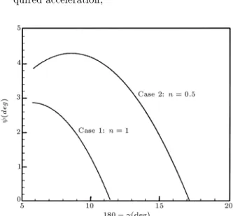
of 500 m. When its distance from a surface target is 5000 m, it res a missile at the target. The missile initial velocity, with respect to the helicopter, is 150 m/s. For the 2-D engagement, one hash= 500 m. The angle between the missile velocity and the LOS versus is shown in Figure 3 for two cases, VO = 150 m/s (Case 1) and 300 m/s (Case 2), respectively. As can be seen, the nal value of becomes zero.

SOLUTION FOR A SPECIAL CASE OF

MANEUVERING TARGET

Consider a special case where a constant-speed ma-neuvering target moves on the surface of a sphere with radius and origin xed at the stationary target tracker. Therefore, one has rt = = vt= and

a

t=; 2

e

r+aht

e

h, in whichahtdepends on the target

motion. Also, = cot;1( ;

2=aht) is dened as the angle between the target acceleration and the LOS.

re-quired acceleration

(7)

2. A constant-speed pursuer.

When a target circles around the target tracker with a constant radius at a constant altitude, which is a special case of moving on the surface of a sphere, one has"="0_= _0andaht=

2tan"

0for _0>0. This case was studied for a constant-speed pursuer in 5] and with the assumption that the pursuer acceleration is equal to the required acceleration in 11].

Case 1: Pursuer Acceleration is Equal to the

Required Acceleration

Consider the pursuer is initially red at the target from the tracker and then maneuvers according to Equations 27, in order to remain on the tracker-target LOS. With the assumption that the pursuer accelera-tion is equal to the required acceleraaccelera-tion, Equaaccelera-tion 11a reduces to rm;rm

2= 0. Therefore, one can derive the following solutions as:

rm= (Vm0=)sinh(t) (68)

Vm=Vm0 p

cosh(2t) (69)

tan = tanh(t): (70)

The pursuer acceleration is also obtained as:

am=Vm0 q

4 + (4 + tan2)sinh

2(t): (71) The pursuer and target positions are equal at the collision instant, therefore,

sinh(tf) = 1=n: (72)

In this case, one must have n > 0 for intercepting the target. The nal values for the pursuer velocity, acceleration and velocity-to-beam angle can then be found as:

Vmf =Vm0 p

1 + (2=n2) (73)

amf=atf = q

1 + (4n2+ 3)cos2

f (74)

tanf = 1=p

n2+ 1: (75)

Case 2: Constant-Speed Pursuer

Consider that the pursuer, with a constant speed, is initially red at the target from the target tracker and then maneuvers according to Equations 27. Note, for this case, arm 6= 0. In other words, the pursuer acceleration is in the direction normal to its velocity vector and the component of the pursuer acceleration normal to the LOS must be equal to the required acceleration. The solution of rm(t) can be found

by rearrangement and integrating the relation _r2

m+

r2

m2=V2

m, with respect to time, that is:

rm= (Vm=)sin(t): (76)

Comparing Equations 42b and 76, the pursuer velocity-to-beam angle can be found as:

= t: (77)

The pursuer acceleration is also obtained as:

am=Vm

q

4 + tan2sin

2(t): (78)

The intercept time is then calculated by:

sin(tf) = 1=n: (79)

The preceding relation implies that the intercept con-dition is n 1. The nal values for the pursuer acceleration and velocity-to-beam angle can also be obtained as:

amf=atf = q

1 + (4n2

;1)cos 2

f (80)

f = sin;1(1=n): (81)

When a target circles around the stationary tracker, one has=;"

0 for _0>0.

CONCLUSIONS

The 3-D equations of LOS guidance with a moving tracker are presented for maneuvering targets. Then, the closed-form solution of the 3-D LOS trajectory of a pursuer for a moving tracker and nonmaneuvering targets is derived with the assumption that the total pursuer acceleration is equal to the required accelera-tion in the direcaccelera-tion normal to the LOS. In this study, the pursuer is always on the line between the target tracker and the target without any error. The present solution can be used in both surface-to-air and air-to-surface applications. In addition, some signicant characteristics, such as total !ight time, cumulative velocity increment, initial conditions for interception and the eects of acceleration limit, are obtained and discussed. The equivalent eective navigation ratio for the LOS guidance is also derived for comparison with TPN guidance law. Finally, the solutions for a special case of a maneuvering target, in which its trajectory is on the surface of a sphere with origin at its tracker, are presented for the two cases with dierent assumptions, namely, a constant-speed pursuer and the pursuer acceleration to be equal to the required acceleration.

(8)

REFERENCES

1. Locke, A.S., Guidance, D. Van Nostrand, Princeton, NJ, USA (1955).

2. Jerger, J.J., System Preliminary Design, D. Van Nos-trand, Princeton, NJ, USA (1960).

3. Garnell, P.,Guided Weapon Control Systems, 2nd Ed., Pergamon Press, Oxford, UK (1980).

4. Macfadzean, R.H.M.,Surface-Based Air Defence Sys-tem Analysis, Artech House, Norwood, MA, USA (1992).

5. Shneydor, N.A.,Missile Guidance and Pursuit: Kine-matics, Dynamics and Control, Horwood Publishing, Chichester, UK (1998).

6. Zarchan, P., Tactical and Strategic Missile Guidance, Progress in Astronautics and Aeronautics,176, AIAA

(1997).

7. Pastrick, P., Seltzer, S.M. and Warren, M.E. \Guid-ance laws for short-range tactical missiles", J. of Guidance and Control,4(2), pp 98-108 (1981).

8. Lin, C.-F.,Modern Navigation, Guidance and Control Processing, Prentice-Hall, Englewood Clis, NJ, USA (1991).

9. Lee, G.T. and Lee, J.G. \Improved command to line-of-sight for homing guidance", IEEE Trans. on Aerospace and Electronic Systems, 31(1), pp 506-510

(1995).

10. Jalali-Naini, S.H. and Esfahanian, V. \Closed-form solution of line-of-sight trajectory for nonmaneuvering

targets", J. of Guidance, Control, and Dynamics,

23(2), pp 365-366 (2000).

11. Jalali-Naini, S.H. and Esfahanian, V. \Closed-form so-lution of 3-D line-of-sight guidance",Proc. of the First International Conference of the Iranian Aerospace So-ciety, Sharif University of Technology, Tehran, I.R. Iran, pp 231-242 (2000-2001).

12. Jalali-Naini, S.H. \Analytical study of a modied LOS guidance", AIAA Navigation, Guidance and Control Conference, Montreal, Canada, Paper No. 2001-4045 (2001).

13. Shoucri, R.M. \Closed-form solution of line-of-sight trajectory for maneuvering targets", J. of Guidance, Control, and Dynamics,24(2), pp 408-409 (2001).

14. Jalali-Naini, S.H. \Approximate solution of 3-D LOS guidance with time-varying velocity," Proc. of the Third Biennial Conference of the Iranian Aerospace Society, Sharif University of Technology, Tehran, I.R. Iran, pp 767-777 (2000-2001).

15. Yang, C.-D. and Yang, C.-C. \Analytical solution of three-dimensional realistic true proportional naviga-tion", J. of Guidance, Control, and Dynamics,19(3),

pp 569-577 (1996).

16. Yang, C.-D. and Yang, C.-C. \Analytical solution of generalized three-dimensional proportional naviga-tion", J. of Guidance, Control, and Dynamics,19(3),