Sharif University of Technology
Scientia IranicaTransactions E: Industrial Engineering www.scientiairanica.com
Interrelating physical and nancial ows in a
bi-objective closed-loop supply chain network problem
with uncertainty
M. Ramezani, A.M. Kimiagari
and B. Karimi
Faculty of Industrial Engineering and Management Systems, Amirkabir University of Technology, Tehran, Iran. Received 25 December 2013; received in revised form 6 April 2014; accepted 2 September 2014
KEYWORDS Closed-loop supply chain;
Finances; Uncertainty;
Multi-objective robust optimization;
Scenario relaxation algorithm.
Abstract. This paper presents a bi-objective logistic design problem integrating the nancial and physical ows of a closed-loop supply chain in which the uncertainty of demand and the return rate are described by a nite set of possible scenarios. The main idea of this paper consists of the joint integration of enterprise nance with the company operations model, where nancial aspects are explicitly considered as exogenous variables. The model addresses the company operations decisions as well as the nance decisions. Moreover, the change in equity is considered as objective function along with the prot to evaluate the business aspects. Since the logistic network design is a strategic problem and the change of conguration is not easy in the future, a bi-objective robust optimization with the max-min version is extended to cope with the uncertainty of parameters. In addition, to obtain solutions with a better time, the scenario relaxation algorithm is adapted for the proposed approach. The numerical examples are presented to show the applicability of the model along with a sensitivity analysis on nancial parameters. The obtained results illustrate the importance of such modelling systems leading to more overall earnings and expressing further insights on the interactions between operations and nances.
c
2015 Sharif University of Technology. All rights reserved.
1. Introduction
Supply Chain Management (SCM) aims to integrate plants with their suppliers, customers and other fa-cilities in network so that they can be managed as a single entity, and to coordinate all input/output ows (of materials, information and funds) so that products are produced and distributed in the right quantities, to the right locations, and at the right time. The recent SCM models in literature, as mentioned by Guillen, Badell, Espu~na and Puigjaner [1], are often focused
*. Corresponding author. Tel.: +98 21 64542228; Fax: +98 21 66959195
E-mail addresses: [email protected] (M. Ramezani); [email protected] (A.M. Kimiagari)
on the physical ows of goods in network including the best location of facilities, the optimum ow of materials/products and optimum value of inventory with respect to the performance measure of cost or prot. However, any SC has in parallel a nancial chain, and aspects related to the analysis of corporate nancial decisions are not considered within these mod-els. Therefore, these models are no longer adequate and must present an optimized plan along with an optimized budget.
On the other hand, Supply Chain Network Design (SCND) problem is an important one in SCM that involves both strategic and tactical decisions. In general, the SCND problem is concerned with the determination of the optimal number, technology, and conguration of the facilities as well as the quantities
of purchasing, production, distribution, inventory, and shipments among the established facilities in such a way to optimize both the customer satisfaction and the chain value. The network in a SCND problem consists of two parts: Forward Logistic (FL) and Reverse Logis-tic (RL). The rst only considers the forward facilities (such as supplier, plant, and distribution center), while the latter considers the backward facilities (such as collection center, repair center, and disposal center). Because designing the forward and reverse logistics sep-arately results in sub-optimal designs with respect to objectives of the supply chain, the Closed-Loop Supply Chain (CLSC) network design is critically important and can guarantee the least waste of materials by following the conservation laws during the life cycle of the materials [2].
Hence, this paper presents an integrated design of closed-loop supply chain interrelating physical and nancial ows with the uncertainty in demands and re-turn rate. The main idea of this paper is to incorporate the nancial issues and a set of budgetary constraints representing balances of cash, debt, securities, payment delays, and discounts in the supply chain planning. In addition, the change in equity is considered as objective function along with the prot to evaluate the SC system. To deal with uncertainty in the parameters, described by a set of possible scenarios, multi-objective robust optimization approach is adapted to solve the proposed model. Besides, to nd a solution with a faster computation time, the scenario relaxation algorithm is presented that performs more eciently compared to the extensive form model. In other words, the main contributions of this paper can be summarized as follows:
Presenting a novel bi-objective closed-loop supply chain design model integrating the nancial ows and the physical ows;
Achieving the applicability and eciency of the scenario relaxation algorithm compared to the ex-tensive form model to solve the SCND model that contemplates the uncertainty of the demand and the return rate as a nite number of possible scenarios.
The structure of this paper is as follows. Section 2 reviews the literature of SCND problem with focus on nancial issues. A mathematical model for design of closed-loop supply chain under uncertainty with the nancial considerations is presented in Section 3. Section 4 addresses multi-objective robust optimization approach and explains the scenario relaxation algo-rithm to achieve a solution with a faster computation time. Section 5 illustrates the numerical examples and discusses the computational results. Finally, we report the conclusions of this paper in Section 6.
2. Literature review
Regarding SCM models, there have been a considerable number of publications in recent years. The rst researches considered linear, product, single-period, deterministic problems. Then, complex, non-linear, multi-product, multi-period, stochastic ones as new constraints were appended to the existing models, in order to yield more realistic ones. Two main streams of literature are relevant to our research:
1. The studies considering the nancial decisions in SCM;
2. The researches associated with closed-loop supply chain.
In the rst stream, incorporation of nancial decisions in SCM, both qualitative and quantitative studies can be observed in the literature. Wang, Batta, Bhadury and Rump [3] addressed a facility location problem with budget constraints in which the opening of new facilities and the closing of existing facilities are considered. The objective of the model is to minimize the distance from customer subject to the restriction of investment budget and number of facilities. Badell, Romero, Huertas and Puigjaner [4] presented a Mixed Integer Linear Programming (MILP) model to im-plement the nancial cross functional links with the enterprise value-added chain, where the activities of planning, scheduling, and budgeting are integrated at plant level. The main contribution of this paper is to incorporate the nancial issues (i.e. budgeting model) into Advanced Planning and Schedule (APS) enterprise systems. Guillen, Badell and Puigjaner [5] presented a mathematical model that optimizes simultaneously activities of scheduling, production planning, and cor-porate nancial planning in a holistic framework. The objective of this paper is to maximize change in equity instead of maximizing prot.
Puigjaner and Guillen-Gosalbez [6] addressed the supply chain optimization at the operation level in the chemical process industry. An integrated ap-proach was suggested for supply chain management in a multi-agent framework. The paper considers supply chain dynamics, the environmental impacts, the business issues, and key performance indicator in the proposed problem. Hammami, Frein and Hadj-Alouane [7] presented a strategic-tactical model for the design of a supply chain network in the delocalization context. The paper considers the logistic decisions, i.e. location of facilities, technology choice, supplier selection, and product ows among chain, as well as the nancial decisions, i.e. transfer pricing and transportation costs allocation. Lanez, Puigjaner and Reklaitis [8] presented a model for supply chain management with focus on the process operations and the Product Development Pipeline Management
(PDPM) problem. The paper addresses the nancial and nancial engineering considerations with inow and outow cash in each period, strategic management of supplier and customer relations by inventory man-agement and option contracts. Protopappa-Sieke and Seifert [9] presented a mathematical model to integrate the operational and nancial supply chain management in the inventory control area. The model decides on the optimal purchasing order quantity with respect to the capital constraints and payment delays while performance measurements of the service level, return on investment, prot margin, and inventory level are analysed in the relevant supply chain. Longinidis and Georgiadis [10] proposed a Mixed Integer Linear Programming (MILP) formulation for design of a supply chain network including plants, warehouses, distribution centers, and customers. The paper extends the existing models in the literature by incorporating the nancial issues as nancial ratios and considering the demand uncertainty. Nickel, Saldanha-da-Gama and Ziegler [11] presented a multi-stage supply chain network design problem in which the decisions of the lo-cation of the facilities, the ow of commodities and the investments to be made in alternative activities to those directly related with the supply chain design. The goal was to maximize the total nancial benet and an alter-native formulation which is based upon the paths in the scenario tree was also proposed. Longinidis and Geor-giadis [12] presented a mathematical model that inte-grates nancial performance and credit solvency mod-elling with SCN design decisions under economic uncer-tainty. The multi-objective Mixed Integer Non-Linear Programming (moMINLP) model enchased nancial performance through economic value added and credit solvency through a valid credit scoring model.
In the second stream, network design in closed-loop supply chain, various studies have addressed this problem in literature. Chan, Kumar and Choy [13] presented a facility location-allocation model for col-lection, reprocessing, and redistribution of carpet to design the location and capacity of a regional recovery center. The model minimized the costs of invest-ment, processing, and transportation. Fleischmann, Beullens, Bloemhof-Ruwaard and Van Wassenhove [2] proposed a SCND model analysing the forward ow to-gether with the return ow. Fleischmann's model was extended by Salema, Barbosa-Povoa and Novais [14] to a multi-product capacitated reverse logistic network with uncertainty in the demands and returns, which was used by an Iberian company. Uster, Easwaran, Akcali and Cetinkaya [15] presented a multi-product close-loop SCND model and considered the production and reproduction separately. They regarded the fea-ture of single sourcing for the customers for a better management of customers. The Benders decomposition method also was used to solve the model.
Ko and Evans [16] developed a dynamic, in-tegrated, closed-loop network operated by the third Party Logistics (3PL) service provider. They applied a Genetic Algorithm (GA) to solve their model. Aras, Aksen and Gonul Tanugur [17] presented a non-linear recovery logistic network design whose objective is to maximize the total prot. The model decided about the locations of collection centers and suitable price for returned products. Moreover, a Tabu search solution procedure was proposed to nd the solution of model. Min and Ko [18] proposed a dynamic design of a reverse SCND problem and presented a GA to solve the problem, including the location and allocation for 3PLs. Salema, Barbosa-Povoa and Novais [19] introduced a multi-product and multi-period model for a supply chain network with reverse ows, where an approach based on graph is applied to model the relevant problem. The model simultaneously integrates the strategic decisions (i.e. network design) and the tactical decisions (i.e. planning of supply chain related to supply, production, storage and distribution).
El-Sayed, Aa and El-Kharbotly [20] proposed a multi-period, multi-echelon, forward-reverse logistics network design model. They considered four layers in the forward direction (i.e. suppliers, plants, dis-tribution centers and customers) and three layers in the return direction (i.e. customers, disassembly and redistribution centers). The objective of their model is to maximize the prot of the supply chain. Pishvaee, Farahani and Dullaert [21] suggested a bi-objective integrated closed-loop supply chain design model in which the costs and the responsiveness of logistic net-work are considered objectives of model. They devel-oped an ecient multi-objective memetic algorithm by applying three dierent local searches in order to nd the set of non-dominated solutions. Wang and Hsu [22] presented a close-loop SCND model that takes into account the locations of plants, distribution centers, and dismantlers as decision variables. The model used the distribution centers as hybrid processing facilities for both the forward and backward ows. In addition, to solve the proposed model, a revised spanning-tree based GA with determinant encoding representation was introduced. Soleimani, Seyyed-Esfahani and Shi-razi [23] proposed a multi-period, multi-product closed-loop supply chain network with stochastic demand and price. A multi criteria scenario based solution ap-proach was then developed to nd an optimal solution through some logical scenarios and three comparing criteria. Mean, Standard Deviation (SD), and Coef-cient of Variation (CV) were the mentioned criteria for nding the optimal solution. Ramezani, Bashiri and Tavakkoli-Moghaddam [24] introduced a multi-objective stochastic model to design a forward/reverse supply chain network under an uncertain environment. The performance of chain is evaluated through three
measures: prot, customer responsiveness, and quality of suppliers (using Six Sigma concept). The Pareto op-timal solutions along with the relevant nancial risk are computed to illustrate tradeos of objectives, and give a proper insight for having a better decision making.
Soleimani, Seyyed-Esfahani and Kannan [25] ad-dressed the design and planning problem of a CLSC in a two-stage stochastic structure. Based on three types of risk measures (i.e. mean absolute devia-tion, value at risk and conditional value at risk), three types of mean-risk models were developed as objective functions, and decision-making procedures were undertaken based on the expected values and risk adversity criteria. The performances of these developed mean-risk models were evaluated in various aspects. Ramezani, Kimiagari, Karimi and Hejazi [26] addressed the application of fuzzy sets to design a multi-product, multi-period, closed-loop supply chain network in which three objective functions (i.e., max-imization of prot, minmax-imization of delivery time, and maximization of quality) are considered. The authors jointly considered fuzzy/exible constraints for fuzziness, fuzzy coecients for lack of knowledge, and fuzzy goal of decision maker(s). Longinidis and Georgiadis [27] introduced a Mixed-Integer Non Linear
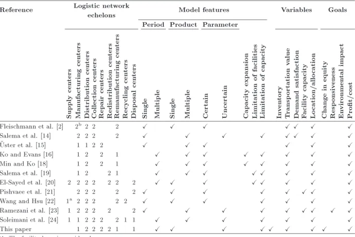
Programming (MINLP) model that integrates sale and leaseback (SLB) technique with SCN design decisions. By exploiting the properties of the MINLP model, it was reformulated into an exact Mixed-Integer Linear Programming (MILP) model that is solved to global optimality. A real case study from a consumer goods company was utilized in order to show model's func-tionality and to evaluate its adaptability, robustness, and benet. Ramezani, Kimiagari and Karimi [28] presented a nancial approach to model a closed-loop supply chain design with the deterministic parameters in which nancial aspects are explicitly considered as exogenous variables. The main contribution of this paper is to incorporate the nancial aspects and a set of budgetary constraints in the supply chain planning. As pointed out by Shapiro [29], Melo, Nickel and Saldanha-da-Gama [30], the nancial consideration is one of the most signicant issues in SCM. However, as can be concluded from the above-mentioned literature, the studies integrating nancial ows with physical product ows in the SCM, especially in the CLSC area, remains scare [31]. A stream of the literature research with a focus on the closed-loop networks was presented in this section. As can be concluded from the above-mentioned literature and also Table 1,
Table 1. Review of the existing studies in closed-loop supply chain network design. Reference Logistic network
echelons Model features Variables Goals
Period Product Parameter
Supply
cen
ters
Man
ufacturing
cen
ters
Distribution
cen
ters
Collection
cen
ters
Repair
cen
ters
Redistribution
cen
ters
Reman
ufacturing
cen
ters
Recycling
cen
ters
Disp
osal
cen
ters
Single Multiple Single Multiple Certain Uncertain Capacit
y
expansion
Limitation
of
facilities
Limitation
of
capacit
y
In
ven
tory
T
ransp
ortation
value
Demand
satisfaction
Facilit
y
capacit
y
Lo
cation/allo
cation
Change
in
equit
y
Resp
onsiv
eness
En
vironmen
tal
impact
Prot/cost
Fleischmann et al. [2] 2b 2 2 2 X X X X X X X
Salema et al. [14] 2 2 2 2 X X X X X X X X
Uster et al. [15] 1 1 2 2 X X X X X X
Ko and Evans [16] 1 2 2 1 X X X X X X X X
Min and Ko [18] 1 2 2 1 X X X X X X X X
Salema et al. [19] 1 2 2 1 X X X X X X X X
El-Sayed et al. [20] 2 2 2 2 2 2 2 X X X X X X X X
Pishvaee et al. [21] 2 2 2 2 2 X X X X X X X X
Wang and Hsu [22] 1a 2 2 2 2 2 X X X X X X X
Ramezani et al. [23] 1 2 2 2 2 2 X X X X X X X X X
Soleimani et al. [24] 1 1 2 2 2 2 1 1 X X X X X X X
This paper 1 2 2 2 2 1 1 X X X X X X X X X
a1: The facility layer is considered.
few studies have considered the nancial aspects in the SCND problems with uncertainty. Moreover, the majority of these studies have considered the nancial aspects as general issues and endogenous, whereas this paper considers the nancial aspects as exogenous variables with details appeared in the constraints and the objective functions. The novelty of this work lies on the integration of nancial issues within a closed loop supply chain network as, to the best of our knowledge, no other study in the eld has made this endeavor.
3. Mathematical model
The model proposed in this paper decided about the facility locations, inventory, and the ows among facilities as well as nancial issues with respect to uncertainty of the demands and return rate. The general structure of the proposed closed-loop logistic network is illustrated in Figure 1. The purpose is to evaluate a closed-loop logistic system with the criteria of prot and change in equity. The following sets, parameters and variables are used in the formulation: Indices:
I Set of plants, i 2 I;
J Set of distribution centers, j 2 J ; E Set of collection centers, e 2 E; H Set of recovery centers, h 2 H; K Set of redistribution centers, k 2 K; F Set of disposal centers, f 2 F; M Set of rst market customer zones,
m 2 M;
N Set of second market customer zones, n 2 N ;
T Set of time periods, t 2 T ; S Set of scenarios, s 2 S. Parameters:
ds
mt Demand of rst customer m in period
t under scenario s
Figure 1. The structure of the proposed supply chain network.
d0s
nt Demand of second customer n in
period t under scenario s;
pmt Price per unit of product for rst
customer m in period t; p0
nt Price per unit of product for second
customer m in period t;
pcit Production cost per unit of product at
plant i in period t;
ocjt Operating cost per unit of product at
distribution center j in period t; icet Inspection and collection cost per unit
of product at collection center e in period t;
rcht Recovery cost per unit of product at
recovery center h in period t;
rdckt Operating cost per unit of product at
redistribution k in period t;
dcft Disposal cost per unit of product at
disposal center f in period t; hcit Holding cost per unit of product at
store of plant i in period t;
dfjt Fixed cost of establishing distribution
center j in period t;
cfet Fixed cost of establishing collection
center e in period t;
rfht Fixed cost of establishing recovery
center h in period t;
rdfkt Fixed cost of establishing redistribution
k in period t;
cpit Production capacity of plant i in
period t;
csit Store capacity of plant i in period t;
cdjt Processing capacity of distribution
center j in period t;
ccet Capacity of collection center e in
period t;
crht Recovery capacity of recovery center h
in period t;
crdkt Redistribution capacity of plant k in
period t;
aijt Transportation cost per unit shipped
from plant i to distribution center j in period t;
bjmt Transportation cost per unit shipped
from distribution center j to rst customer m in period t;
cmet Transportation cost per unit shipped
from rst customer m to collection center e in period t;
deht Transportation cost per unit shipped
from collection center e to recovery center h in period t;
geft Transportation cost per unit shipped
from collection center e to disposal center f in period t;
uhjt Transportation cost per unit shipped
from recovery center h to distribution center j in period t;
vhkt Transportation cost per unit shipped
from recovery center h to redistribution center k in period t;
oknt Transportation cost per unit shipped
from redistribution center k to second customer n in period t;
rs
t Return ratio of used product in period
t under scenario s;
rrt Recovery ratio of used product in
period t;
rst Disposal ratio of used product in
period t;
rdt Redistribution ratio of used product
for rst customer in period t; ret Redistribution ratio of used product
for second customer in period t divt Dividends in period t;
otherst Other net cash obtained in period t;
maxcrd Maximum debt allowed from bank; mincash Minimum cash imposed from bank; scut Marketable securities of initial portfolio
maturing in period t;
The face value of accounts receivable pledged;
tt0 Technical coecient related to
investment of marketable securities; tt0 Technical coecient related to sale of
marketable securities;
'tt0 Technical discount coecient relevant
to the payment of production costs executed in period t incurred in period t0;
tt0 Technical discount coecient relevant
to the payment of handling costs executed in period t incurred in period t0;
%tt0 Technical discount coecient relevant
to the payment of transportation costs executed in period t incurred in period t0.
Decision variables: s
it Quantity of product produced at plant
i in period t under scenario s; s
ijt Quantity of product shipped from
plant i to distribution center j in period t under scenario s;
s
jmt Quantity of product shipped from
distribution center j to rst customer m in period t under scenario s; s
met Quantity of returned product shipped
from rst customer m to collection center e in period t under scenario s; s
eht Quantity of returned product shipped
from collection center e to recovery center h in period t under scenario s; s
eft Quantity of returned product shipped
from collection center e to disposal center f in period t under scenario s; s
hjt Quantity of returned product shipped
from recovery center h to distribution center j in period t under scenario s; s
hkt Quantity of returned product shipped
from recovery center h to redistribution center k in period t under scenario s; s
knt Quantity of returned product shipped
from redistribution center k to second customer n in period t under scenario s;
s
it Quantity of product shipped from
plant i to its store in period t under scenario s;
qs
ijt Quantity of product shipped from
store of plant i to distribution center j in period t under scenario s;
Invs
it Residual inventory at store of plant i
in period t under scenario s; cashs
t Cash in period t under scenario s;
exncashst Exogenous cash in period t under scenario s;
crdcasht Net cash obtained by money borrowed
or repaid to the credit line in period t under scenario s;
scucasht Net cash received or paid in securities
transactions in period t under scenario s;
ppays
tt0 Payment for total costs of production
executed in period t on accounts payable incurred in period t0 under
scenario s; hpays
tt0 Payment for total costs of handling
product in facilities executed in period t on accounts payable incurred in period t0 under scenario s;
tpays
tt0 Payment for total costs of
transportation executed in period t on accounts payable incurred in period t0
under scenario s; recs
t Accounts receivable in period t under
plgs
tt0 Amount of accounts receivable pledged
within period t0 incurred in period t;
crdlinet Debt in period t under scenario s;
loant Amount of cash borrowed to credit line
in period t under scenario s;
repayt Amount of cash repaid to credit line in
period t under scenario s;
iscut0t Total cash obtained in period t0 by
the marketable securities invested in period t under scenario s;
cscut0t Total marketable securities sold in
period t maturing in period t0 under
scenario s; pexpnss
t Expense of production in period t
under scenario s; hexpnss
t Expense of handling product in
facilities in period t under scenario s; texpnss
t Expense of transportation in period t
under scenario s;
fexpnst Expense of establishing facilities in
period t under scenario s; iexpnss
t Expense of holding inventory in stores
in period t under scenario s; Es Expected change in equity of
enterprise;
SAs Expected change in short-term asset of
enterprise;
LAs Expected change in long-term asset of
enterprise;
Ls Expected change in liabilities of
enterprise;
prots Expected prot of enterprise.
Xj=
8 > < > :
1 if distribution center j is established; 0 otherwise;
Ye=
8 > < > :
1 if collection center e is established, 0 otherwise;
Zh=
8 > < > :
1 if recovery center h is established, 0 otherwise;
Wk=
8 > < > :
1 if redistribution center k is established, 0 otherwise;
In terms of the above-mentioned notations, the pro-posed multi-echelon closed-loop logistic network design
problem can be categorized according to balance of physical ow, facilities capacity, balance of nancial ow, and interrelated relations.
3.1. Balance of physical ows s
it=
X
j
s
ijt+ sit; 8i; t; s; (1)
s
it+ Invi(t 1)s =
X
j
qs
ijt+ Invits; 8i; t; s; (2)
X i s ijt+ X i qs ijt+ X h s hjt= X m s
jmt; 8j; t; s; (3)
X
m
s
jmt= dsmt; 8m; t; s; (4)
X
e
s
met= rstdsmt; 8m; t; s; (5)
X h s eht = X m s
metrrt; 8e; t; s; (6)
X m s met= X h s eht+ X f s
eft; 8e; t; s; (7)
X j s hjt= X e s
ehtrdt; 8h; t; s; (8)
X e s eht = X j s hjt+ X k s
hkt; 8h; t; s; (9)
X h s hkt= X n s
knt; 8k; t; s; (10)
X
k
s
knt = d0snt; 8n; t; s; (11)
Constraint (1) shows the production volume for each plant is equal to the sum of the good ow from the plant to all distribution centers and from the plant to its store. Constraint (2) shows, for each plant and in each period, sum of the good ow from the plant to its store and the residual inventory form previous period is equal to the sum of the good ow from the plant store to all distribution centers and the existing residual inventory. Constraint (3) shows, for each distribution center and in each period, sum of the good ow from all plants, plant stores, and recovery centers to the distribution center is equal to the sum of the good ow from the distribution center to all rst market customers. Constraint (4) states that the demand of each rst market customer must be satised in each period. Constraint (5) relates the returned ow to demand of rst market customers in each period. Constraints (6) and (7) show the
returned ows from collection center to the recovery and disposal centers, respectively. Constraint (8) relates the returned ow from collection center to the returned ow to distribution center in each period. Constraints (9)-(11) conduct the returned ows to the redistribution centers, and second customer zones. 3.2. Facilities capacity
s
it cpit; 8i; t; s; (12)
Invs
it csit; 8i; t; s; (13)
X
m
s
jmt cdjtXj; 8j; t; s; (14)
X
h
s eht+
X
f
s
eft ccetYe; 8e; t; s; (15)
X
j
s hjt+
X
k
s
hkt crhtZh; 8h; t; s; (16)
X
n
s
knt crdktWk; 8k; t; s: (17)
Constraint (12) restricts the production value to the capacity of relevant plant. Constraint (13) shows the capacity of plant store in each time period. Constraints (14)-(17) show the capacity of distribution center, collection center, recovery center, and redistribution center, respectively.
3.3. Balance of nancial ows cashst =cashst 1+ exncashst+ crdcasht
+ scucasht fexpnst
X
t0t
ppays tt0
X
t0t
hpays tt0
X
t0t
tpays tt0 divt
+ otherst; 8t; s; (18)
exncashs
t =recst tdel
X
t tdelt0<t
plgs t tdelt0
+ X
t tdel<t0t
plgs
t0t: ; 8t; s; (19)
X
tt0<t+tdel
plgs
tt0 recst; 8t; s; (20)
crdLinet=crdlinet 1+ loant repayt
+ ir:crdlinet 1; 8t; (21)
crdcasht= loant repayt; 8t; (22)
crdlinet maxcrd; 8t; (23)
casht mincash; 8t; (24)
scucasht=scut
X
t0>t
iscut0t+
X
t0>t
cscut0t
+X
t0<t
iscutt0:(1 + tt0)
X
t0<t
cscutt0:(1 + tt0); 8t; (25)
X
t0<t
cscutt0:(1 + tt0) scut
+X
t0<t
iscutt0:(1 + tt0); 8t; (26)
X
t0t
't0t:ppayst0t pexpnsst; 8t; (27)
X
t0t
t0t:hpayst0t hexpnsst; 8t; (28)
X
t0t
&t0t:tpayts0t texpnsst; 8t: (29)
Constraint (18) states that the cash in each period is computed based on the cash in previous period, exogenous cash derived from the sales of products, and the pledging of accounts receivables, net cash obtained by money borrowed or repaid to the credit line, net cash received or paid in securities transactions, payment for costs related to facilities, dividends, and net cash resulted from any other source. Constraint (19) shows that the exogenous cash in each period is equal to the sum of the accounts receivable belonged to period of t tdel matured in period t, minus total amount of the
accounts receivable pledged within period t tdelto t 1
belonged to periods t tdel, plus the cash derived from
pledging of accounts receivable belonged to periods t tdel+1 to t matured in period t. Constraint (20) states
that the total amount of accounts receivable belonged to periods t pledged within period t to t + tdel 1
cannot exceed the amount of accounts receivable in period t.
Constraint (21) states that the total debt in each period is a function of the debt in the previous period, cash borrowed to credit line, cash repaid to credit line, and the interest costs, where Net cash obtained by money borrowed or repaid to the credit line is dened as Constraint (22). In addition to pledging, loan borrowed from bank is another nancing source, obtained at the beginning of period with annual interest rate (ir) under an agreement with the bank. In this case, the
bank imposes rm to have minimum cash, usually as percentage of the amount borrowed, and also restricts rm to an open line of credit. Constraints (23) and (24) show the minimum cash and the maximum credit agreed with the bank.
Constraint (25) shows that, in each period, the cash relevant to the securities transactions is computed as sum of the cash derived from the marketable securi-ties of initial portfolio, minus the cash invested as the marketable securities in the current period, plus the cash resulted from the sale of the marketable securities in the current period, plus total cash obtained in the current period by the marketable securities invested in previous periods with regard to technical coe-cient of investment (tt0), and minus total marketable
securities sold in previous periods maturing in the current period with regard to technical coecient of sale (tt0). Constraint (26) states that, in each period,
total marketable securities sold in previous periods, maturing in the current period, cannot exceed the sum of the cash derived in the current period from the marketable securities of initial portfolio and total cash obtained in the current period by the marketable securities invested in previous periods. Finally, con-straints (27)-(29) show the payments associated with production, handling, and transportation with regard to the relevant expenses.
3.4. Interrelated relations pexpnss
t =
X
i
s
it:pcit; 8t; s; (30)
hexpnss t = X j X m s
jmt:ocjt+
X
m
X
e
s met:icet
+X
e
X
h
s
eht:rcht+
X
h
X
k
s hkt:rdckt
+X
e
X
f
s
eft:dcft; 8t; s; (31)
texpnss t = X i X j (s
ijt+ qsijt):aijt+
X
i
s it:a0it
+X
j
X
m
s
jmt:bjmt+
X
m
X
e
s met:cmet
+X
e
X
h
s
eht:deht+
X
e
X
f
s eft:geft
+X
h
X
j
s
hjt:uhjt+
X
h
X
k
s hkt:vhkt
+X
k
X
n
s
knt:oknt; 8t; s; (32)
fexpnst=
X
j
Xj:dfjt+
X
e
Ye:cfet+
X
h
Zh:rfht
+X
k
Wk:rdfkt; 8t; (33)
iexpnss t=
X
i
Invs
it:hcit; 8t; s; (34)
recs t = X j X m
pmt:jmts +
X
k
X
n
p0
nt::knts ; 8t; s;
(35) SAs=cashs
T+
X
T t<tdel
recs t
X
t;t0jT ttdel^t0>T tdel
plgs tt0
+X
i
Invs
iT:pciT cashst0 rec
s t0
X
i
Invs
it0:pcit0; (36)
LAs=X t
fexpnst fexpnst0; (37)
Ls=crdline T+ X t pexpnss t+ X t hexpnss t +X t texpnss t X tt0
'tt0:ppaystt0
X
tt0
tt0:hpaystt0
X
tt0
&tt0:tpaystt0 crdlinet0:
(38) To determine the outows of cash required to compute the prot and the equity, the expense of production, handling, transportation, establishing facilities, and holding inventory are dened as Constraints (30)-(34), respectively. Constraint (35) shows that, in each period, the accounts receivable is dened as the sale of nal products to the customers in the same period. The change in short-term assets is equal to the dierence between the short-term assets (including the cash available, accounts receivable, and inventory) at the end of rst period and last period presented as Constraint (36). In this equation, the inventory value is computed based on the Generally Accepted Accounting Principles (GAAP) of historic cost, i.e. the lowest price that is production price. Constraint (37) shows the change in long-term assets as sum of expenses of establishing facilities at the end of last period minus the expenses of establishing facilities at the end of the rst period. Constraint (38) states that the change in liabilities is equal to the dierence between the short-term and long-short-term liabilities at the end of the rst
period and the last period including the debts and accounts payable related to the production, handing, and transportation.
3.5. Objective functions profits=X
j
X
m
X
t
pmt:sjmt+
X
k
X
n
X
t
p0 nt::knts
X
t
pexpnss t
X
t
hexpnss t
X
t
texpnss t
X
t
iexpnss t
fexpnst; 8s; (39)
Es= SAs+ LAs Ls; 8s: (40)
The rst objective is the prot that is equal to the total income associated with the sales of products in customer zones minus the total cost associated with the expenses of production, processing, inventory, and transportation expressed by Eq. (39). Traditionally, the decisions related to design/planning and nancial issues are measured in isolated environments. The more common objectives traditionally used in the literature is maximization of the prot or minimization of the cost. However, the nancial community has been for years making decisions taking into account other criteria, such as market to book value, liquidity ratios, capital structure ratios, return on equity, sales margin, turnover ratios, stock security ratios, etc. Nevertheless, second objective function considers the direct enhancement of the shareholder's value as the change in equity expressed by Eq. (40).
4. Multi-objective robust optimization
Robust optimization approaches include the min-max and min-max regret versions dened by Kouvelis and Yu [32]. Let S be a nite set of scenarios and x denote the feasible solution of a given problem. For a minimization problem, Zs(x) and Zs denote the
objective and the optimal objective of problem under scenario s (where s 2 S), respectively. The goal of the min-max version is to nd a solution with the best worst case value across all possible scenarios, which can be stated by:
min
x2Xmaxs2S Zs(x):
In the min-max regret version, the regret value of each scenario is dened by the dierence between the objective value of the feasible solution (i.e., Zs(x)) and
the optimal objective value (i.e., Z
s). This dierence
can be dened by the absolute regret or relative regret.
The goal of the min-max regret and the min-max relative regret is to nd a robust solution minimizing its maximum regret and its maximum relative regret, respectively, which can be formulated by:
min
x2Xmaxs2S Zs(x) Z s;
min
x2Xmaxs2S
Zs(x) Zs
Z s :
Indeed, the corresponding max-min and min-max re-gret version can be dened for maximization problems. Aissi, Bazgan and Vanderpooten [33] addressed the min-max regret and min-max relative regret ap-proaches and presented a comprehensive discussion of the incentives for developing these approaches and diverse aspects of employing robust optimization in practice. Chan, Kumar and Choy [13], Ben-Tal and Nemirovski [34] were engaged in robust opti-mization, by allowing the data to be ellipsoids, and proposed ecient algorithms to solve convex opti-mization problems under data ambiguity. Gumus and Guneri [35], Bertsimas and Sim [36] presented an approach for discrete optimization and network ow problems that provides the degree of conser-vatism of the solution to be handled. They demonstrated that the robust equivalent of an NPhard -approximable 0-1 discrete optimization problem stays -approximable.
In addition, some approaches have been proposed to reduce the number of scenarios. Lee, Chiu, Yeh and Huang [37] proposed an -reliable min-max regret model to nd a solution minimizing the problem with regard to a selected subset of scenarios whose occurrence probability is greater than the user-specied value . Moussawi-Haidar and Jaber [38] suggested another approach, called lexicographic -robustness, which considers all scenarios in the lexicographic order from the worst to the best, instead of considering the worst case scenario. This approach incorporates a tolerance threshold, , so not to dierentiate among solutions with similar values. Assavapokee, Real, Ammons and Hong [39] presented a scenario relaxation algorithm for the max regret version and the min-max relative regret version. The algorithm iteratively solves and updates a series of relaxed sub-problems so that both the feasibility and optimality conditions of the problem are satised.
The proposed model in this study assumes that the demand and the return rate are uncertain, intro-duced by a nite set of possible scenarios with unknown joint probability distribution. To obtain a Pareto solution of the proposed model, we use the -constraint method presented by Wang, Fu, Lee and Zeng [40]. This method is one of the multi-objective techniques with priori articulation of DM's preference information
and is a one-stage technique with computationally fast time. The method is based on optimization of one objective function and considering the other objectives as constraint with allowable worst bound. Then, the bound is consecutively modied to generate the other Paretooptimal solutions. Corresponding to the -constraint method, the robust multi-objective closed-loop SCND problem with the best worst case value across all possible scenarios is formulated as follows:
min s.t.
fs
1(V; Qs)
fs
2(V; Qs) g2
Eqs. (1)-(38) 9 > > > > > > = > > > > > > ;
8s 2 S; (41)
where f1
s is the rst objective function under scenario
s; g2 is the desired worst of second objective function;
V is the set of rst-stage variables; and Qsis the set of
second-stage variables, where, decision variables have to be taken before the realization of the uncertainty and the second-stage variables will be made after the uncertain parameters have been revealed.
Unfortunately, the size of the model presented in Relation (41), referred as the extensive form model under deviation robust denition, can become unman-ageably large when a large number of scenarios are considered. The implementation of this model requires a vigorous computational time to obtain a robust solution with a large number of scenarios. For this reason, we use the scenario relaxation algorithm to obtain a solution with a better time. In the algorithm, the optimal rst objective function of each scenario is necessarily resulted by solving the following model.
f1 s =
8 > > > < > > > :
max fs 1(V; Qs)
s.t. fs
2(V; Qs) g2
Eqs. (1)-(38)
(42)
The main idea of the scenario relaxation algorithm is that in a problem with a large number of possible scenarios only a small subset of scenarios actually is employed to nd an optimal solution. Initially, the algorithm solves the problem for a subset of scenarios (sub-problems) and then sequentially searches to ex-amine all possible scenarios. The algorithm adds those scenarios that disturb the optimality and/or feasibility conditions to the sub-problem. It is showed that the algorithm stops at an optimal robust solution (if one exists) in a nite number of iterations. The overall procedure of the scenario relaxation algorithm for the max-min version can be summarized as follows.
Step 0: Select a subset S S, set LB = 1 and UB = 0, determine a predetermined small nonnegative value ", and then proceed to Step 1. Here subset S randomly is selected and its cardinality is two. Moreover, value of " is equal to zero.
Step 1: Solve the relaxed model considering only the scenario set S instead of S. If the relaxed model is infeasible, the algorithm is ended (i.e., no robust solution exists). Otherwise, set UB = (i.e., the optimal value of
the relaxed model) and x the rst-stage variables in the current solution form of the relaxed model. If LB UB ", the resulting robust solution is globally "-optimal robust solution, and algorithm is ended. Otherwise, proceed to Step 2.
Step 2: Solve the general model for each scenarios Sn S. Let S1 n S such that the model is
infeasible and let S2 Sn( S [ S1 such that
f1
s (V; Qs) .
Step 3: If S1 6= ; proceed to Step 4. Otherwise,
update the lower bound of algorithm as follows.
LB max(LB; min
s2S(f 1
s (V; Qs))):
If LB UB ", the resulting robust solution is globally "-optimal robust solution and algorithm is ended. Otherwise, proceed to Step 5.
Step 4: Choose a subset S0
1 S1, add to scenario
set S, and then proceed to Step 1. Here, we randomly select subset S0
1with cardinality 2
as algorithm confronts the scenarios in which model is infeasible.
Step 5: Choose a subset S0
2 S2, add to scenario
set S, and then proceed to Step 1. Here, we select subset S0
2 with cardinality 1 as value
of f1
s (V; Qs) is minimum, although it can be
randomly selected.
5. Computational results
To demonstrate the verication and practicality, we consider several test problems to analyse the proposed supply chain system. The sizes of these test problems are illustrated in Table 2. The proposed closed-loop supply chain involves two echelons in forward direction related to the plants, distribution centers, and rst customers as well as four echelons in backward direc-tion related to the collecdirec-tion centers, recovery centers, redistribution centers, disposal centers, and second cus-tomers. The plants are responsible for producing the
Table 2. Size of test problems.
Problem code jIj jJ j jEj jHj jKj jFj jMj jN j jT j
2-3-3-3-2-2-5-3-5 2 3 3 3 2 2 5 3 5
3-5-4-4-3-2-10-5-5 3 5 4 4 3 2 10 5 5
4-6-4-4-3-3-15-8-5 4 6 4 4 3 3 15 8 5
5-7-4-4-3-3-20-5-10 5 7 4 4 3 3 20 5 10
7-10-6-5-4-3-25-8-10 7 10 6 5 4 3 25 8 10
8-12-7-6-6-4-30-10-10 8 12 7 6 6 4 30 10 10
new product to rst customer shipped via distribution centers. In backward direction, the returned products from customers are shipped to collection centers to inspect. If the returned product is recoverable, it is shipped to the recovery center; otherwise, it is shipped to the disposal center. After shipping the recoverable products to recovery centers, depending on the quality of the recovered products, they are shipped to distribution or redistribution centers.
Table 3 illustrates the parameters used in the test
Table 3. Values of parameters used in the test problems.
Parameter Value
d Uniform (400, 650)
d0 Uniform (170, 260)
p Uniform (230, 320)
p0 Uniform (140, 210)
pc Uniform (25, 35)
oc Uniform (10, 15)
ic Uniform (3, 7)
rc Uniform (8, 16)
rdc Uniform (9, 15)
dc Uniform (4, 9)
hc Uniform (4, 9)
df Uniform (30,000, 45,000) cf Uniform (10,000, 15,000) rf Uniform (15,000, 20,000) rdf Uniform (12,000, 16,000)
cp Uniform (750, 900)
cs Uniform (150, 250)
cd Uniform (550, 750)
cc Uniform (450, 600)
cr Uniform (250, 350)
crd Uniform (200, 300) a; b; c; d; g; u; v; o Uniform (2, 9)
r Uniform (0.35, 0.55)
rr Uniform (0.6, 0.9)
rs 1-rr
rd Uniform (0.5, 0.65)
re 1-rd
problems. The initial cash is equal to 300000, where the minimum cash in each period is equal to 120000. Moreover, an open line of credit with a maximum debt of 100000 is allowed in each period. Table 4 shows the initial portfolio of marketable securities investment. The price of the inventories at the end of the time pe-riod is the lowest price, i.e. the production price. The products sold in each period are paid with a delay of 2 time periods and the account receivables are pledged at 80% of their value. Moreover, liabilities borrowed due to the costs of production, processing in facilities must be repaid within 3 time period (2%: 1 time period, net-3 time periods), where technical coecients ('tt0,
tt0 and %tt0) introduce the relevant term. Thus, the
discount can be obtained if the payments are executed timely, otherwise the discount cannot be acquired. The payments related to the transportation services cannot be stretched, and must be executed within the same period of time. Associated with technical coecients and with transactions of marketable securities, a 2.8% annual interest for purchases and a 3.5% one for sales are assumed. Outows withdrawn from the company, as dividends at the end of the time horizon, as well as outows due to payrolls, tax, wages, rents, changes in xed assets, and the repayment of the long-term debt during the whole time horizon are also considered. It is assumed that each uncertain parameter can varies from 80% to 120% of the values in the deterministic model that is dened by a nite number of possible scenarios. The number of possible scenarios also varies from 20 to 150 scenarios in each test problem. The test problems were coded using GAMS and CPLEX solver with " = 0 on a computer with an Intel core2 Duo 2.00 GHz processor and 2.00 GB of RAM.
To evaluate the proposed model, rst, we consider the test problem 1 with Gap 0. Figure 2 shows trade-o between the prot and the change in equity as a Pareto curve, while the number of scenarios is equal to 20. As can be seen in Figure 2, the prot decreases with increase of the change in equity. In addition, a sensitivity analysis of demand is shown in Figure 2, where with increase of demand, both, the change in equity and the prot increase, as well as with decrease of demand, the objectives decrease. This Pareto curve helps the decision maker(s) for a better
Table 4. Marketable securities of initial portfolio. Time periods
t1 t2 t3 t4 t5 t6 t7 t8 t9 t10
Initial portfolio 40000 30000 21000 15000 12000 25000 20000 35000 8000 27000
Figure 2. Change in equity versus prot.
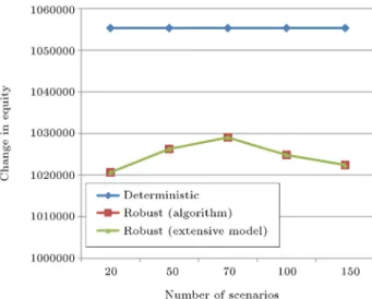
Figure 3. Change in equity for the dierent modes.
analysis. Moreover, Figure 3 shows the behavior of objective function of the change in equity under the dierent scenarios. The value of change in equity for the robust mode computed by both the extensive model and the scenario relaxation algorithm is less than the deterministic mode; this is reasonable because the robust approach optimizes the worst-case scenario. As can be seen in Figure 3, the values of the change in equity for the extensive model and the scenario relaxation algorithm is the same. It is proved that the scenario relaxation algorithm produces an optimal solution, of course with a better time.
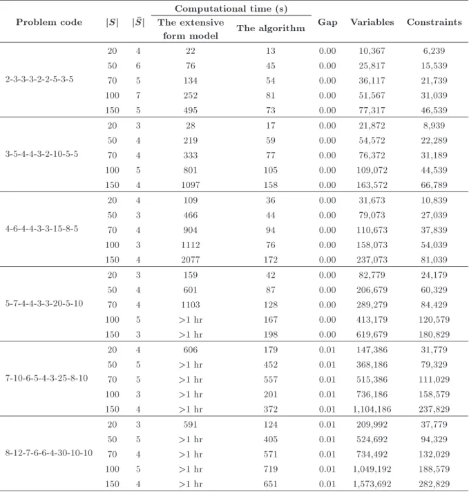
On the other hand, to illustrate the applicability of the scenario relaxation algorithm, six test problems with various scenarios are evaluated only by the change
in equity; the relevant results are reported in Table 4. If the extensive model does not obtain a solution within 1 hour, the computational time is reported as \> 1 hr" in this table. As can be observed, the number of constraints and variables of test problems increase with increment in the number of scenarios. As the results show, the scenario relaxation algorithm dominates the extensive model in all test problems with respect to the computational time; especially this superiority is more signicant when the scale of test problems and the number of scenarios are increased. Table 5 also shows the number of scenarios actually used by the scenario relaxation algorithm (i.e., j Sj) to nd an optimal solution. Increase (or decrease) in number of these scenarios proportionally increases (or decreases) the computational time of the scenario relaxation algorithm. For example, in test problem 3, the computational time of algorithm, for instance with 70 scenario, is greater compared, for instance, with 100 scenario; this is because the number of scenarios employed by the algorithm for instance with 70 sce-nario, is more compared for instance with 100 scenario. According to the previous discussion, the results are consistent and obviously show the benet of using the scenario relaxation algorithm over the extensive model. These results, which are good improvements, convince the decision makers to employ the scenario relaxation algorithm.
6. Conclusion
This paper has presented a model integrating the nancial ows with the physical ows in the design of a closed-loop supply chain in which the eective measure based on an economic performance indicator (i.e. the change in equity) in addition to the commonly used prot is regarded. The model also has considered the uncertainty in demand and return rate through scenario, which assign the occurring possibilities on each scenario. This approach enables the supply chain managers to forecast their demands and return rate as well as to modify their wrong forecasts. To cope with the uncertainty, the robust optimization was employed in the proposed model. Moreover, to nd a robust solu-tion with better time, the scenario relaxasolu-tion algorithm was extended to a max-min version and for multiple objectives. The results showed a successful design of the proposed closed-loop logistic network as well as an obvious performance of the scenario relaxation algorithm on the given problems.
Table 5. Computational results for test problems. Problem code jSj j Sj
Computational time (s)
Gap Variables Constraints The extensive
form model The algorithm
2-3-3-3-2-2-5-3-5
20 4 22 13 0.00 10,367 6,239
50 6 76 45 0.00 25,817 15,539
70 5 134 54 0.00 36,117 21,739
100 7 252 81 0.00 51,567 31,039
150 5 495 73 0.00 77,317 46,539
3-5-4-4-3-2-10-5-5
20 3 28 17 0.00 21,872 8,939
50 4 219 59 0.00 54,572 22,289
70 4 333 77 0.00 76,372 31,189
100 5 801 105 0.00 109,072 44,539
150 4 1097 158 0.00 163,572 66,789
4-6-4-4-3-3-15-8-5
20 4 109 36 0.00 31,673 10,839
50 3 466 44 0.00 79,073 27,039
70 4 904 94 0.00 110,673 37,839
100 3 1112 76 0.00 158,073 54,039
150 4 2077 172 0.00 237,073 81,039
5-7-4-4-3-3-20-5-10
20 3 159 42 0.00 82,779 24,179
50 4 601 87 0.00 206,679 60,329
70 4 1103 128 0.00 289,279 84,429
100 5 >1 hr 167 0.00 413,179 120,579
150 3 >1 hr 198 0.00 619,679 180,829
7-10-6-5-4-3-25-8-10
20 4 606 179 0.01 147,386 31,779
50 5 >1 hr 452 0.01 368,186 79,329
70 5 >1 hr 557 0.01 515,386 111,029
100 3 >1 hr 201 0.01 736,186 158,579
150 4 >1 hr 372 0.01 1,104,186 237,829
8-12-7-6-6-4-30-10-10
20 3 591 124 0.01 209,992 37,779
50 5 >1 hr 405 0.01 524,692 94,329
70 4 >1 hr 571 0.01 734,492 132,029
100 5 >1 hr 719 0.01 1,049,192 188,579
150 4 >1 hr 651 0.01 1,573,692 282,829
As a result, incorporating the nancial ow helps DM(s) to take holistic decisions in order to guarantee new funds from shareholders and nancial institutions that will permit the continuously nancing of com-pany's operations. Moreover, related to performance measures, a decision making process, that does not consider both these measures, may result in congu-ration which performs well only one of the objectives, but performs poorly the other objectives. Hence, the trade-o between these measures, as a Pareto curve, is a useful tool for the supply chain managers to make a proper decision. Finally, it should be pointed out that incorporating other issues related to the product portfolio theory, game theory, future contracts, and
sell techniques in model can be considered as future research.
Acknowledgment
The authors would like to thank the Ghalamchi Cul-tural Foundation that nancially supported this re-search.
References
1. Guillen, G., Badell, M., Espu~na, A. and Puigjaner, L. \Simultaneous optimization of process operations and nancial decisions to enhance the integrated
plan-ning/scheduling of chemical supply chains", Comput-ers and Chemical Engineering, 30(3), pp. 421-436 (2006).
2. Fleischmann, M., Beullens, P., Bloemhof-Ruwaard, J.M. and Van Wassenhove, L.N. \The impact of product recovery on logistics network design", Produc-tion and OperaProduc-tions Management, 10(2), pp. 156-173 (2001).
3. Wang, Q., Batta, R., Bhadury, J. and Rump, C.M. \Budget constrained location problem with opening and closing of facilities", Computers and Operations Research, 30(13), pp. 2047-2069 (2003).
4. Badell, M., Romero, J., Huertas, R. and Puigjaner, L. \Planning, scheduling and budgeting value-added chains", Computers and Chemical Engineering, 28(1-2), pp. 45-61 (2004).
5. Guillen, G., Badell, M. and Puigjaner, L. \A holistic framework for short-term supply chain management integrating production and corporate nancial plan-ning", International Journal of Production Economics, 106(1), pp. 288-306 (2007).
6. Puigjaner, L. and Guillen-Gosalbez, G. \Towards an integrated framework for supply chain management in the batch chemical process industry", Computers and Chemical Engineering, 32(4-5), pp. 650-670 (2008).
7. Hammami, R., Frein, Y. and Hadj-Alouane, A.B. \A strategic-tactical model for the supply chain design in the delocalization context: Mathematical formulation and a case study", International Journal of Production Economics, 122(1), pp. 351-365 (2009).
8. Lanez, J.M., Puigjaner, L. and Reklaitis, G.V. \Fi-nancial and \Fi-nancial engineering considerations in sup-ply chain and product development pipeline manage-ment", Computers and Chemical Engineering, 33(12), pp. 1999-2011 (2009).
9. Protopappa-Sieke, M. and Seifert, R.W. \Interrelating operational and nancial performance measurements in inventory control", European Journal of Operational Research, 204(3), pp. 439-448 (2010).
10. Longinidis, P. and Georgiadis, M.C. \Integration of nancial statement analysis in the optimal design of supply chain networks under demand uncertainty", In-ternational Journal of Production Economics, 129(2), pp. 262-276 (2011).
11. Nickel, S., Saldanha-da-Gama, F. and Ziegler, H.-P. \A multi-stage stochastic supply network design problem with nancial decisions and risk management", Omega, 40(5), pp. 511-524 (2012).
12. Longinidis, P. and Georgiadis, M.C. \Managing the trade-os between nancial performance and credit solvency in the optimal design of supply chain networks under economic uncertainty", Computers & Chemical Engineering, 48, pp. 264-279 (2013).
13. Chan, F.T.S., Kumar, N. and Choy, K.L.
\Decision-making approach for the distribution centre location problem in a supply chain network using the fuzzy-based hierarchical concept", Proceedings of the Insti-tution of Mechanical Engineers, Part B: Journal of Engineering Manufacture, 221(4), pp. 725-739 (2007).
14. Salema, M.I.G., Barbosa-Povoa, A.P. and Novais, A.Q. \An optimization model for the design of a capacitated multi-product reverse logistics network with uncer-tainty", European Journal of Operational Research, 179(3), pp. 1063-1077 (2007).
15. Uster, H., Easwaran, G., Akcali, E. and Cetinkaya, S.
\Benders decomposition with alternative multiple cuts for a multi-product closed-loop supply chain network design model", Naval Research Logistics, 54(8), pp. 890-907 (2007).
16. Ko, H.J. and Evans, G.W. \A genetic algorithm-based heuristic for the dynamic integrated forward/reverse logistics network for 3PLs", Computers and Operations Research, 34(2), pp. 346-366 (2007).
17. Aras, N., Aksen, D. and Gonul Tanugur, A. \Locat-ing collection centers for incentive-dependent returns under a pick-up policy with capacitated vehicles", European Journal of Operational Research, 191(3), pp. 1223-1240 (2008).
18. Min, H. and Ko, H.J. \The dynamic design of a reverse logistics network from the perspective of third-party logistics service providers", International Journal of Production Economics, 113(1), pp. 176-192 (2008).
19. Salema, M.I.G., Barbosa-Povoa, A.P. and Novais, A.Q. \Simultaneous design and planning of supply chains with reverse ows: A generic modelling framework", European Journal of Operational Research, 203(2), pp. 336-349 (2010).
20. El-Sayed, M., Aa, N. and El-Kharbotly, A. \A
stochastic model for forward-reverse logistics network design under risk", Computers and Industrial Engi-neering, 58(3), pp. 423-431 (2010).
21. Pishvaee, M.S., Farahani, R.Z. and Dullaert, W. \A memetic algorithm for bi-objective integrated for-ward/reverse logistics network design", Computers and Operations Research, 37(6), pp. 1100-1112 (2010).
22. Wang, H.F. and Hsu, H.W. \A closed-loop logistic model with a spanning-tree based genetic algorithm", Computers and Operations Research, 37(2), pp. 376-389 (2010).
23. Soleimani, H., Seyyed-Esfahani, M. and Shirazi, M. \A new multi-criteria scenario-based solution approach for stochastic forward/reverse supply chain network design", Annals of Operations Research, pp. 1-23 (2013).
24. Ramezani, M., Bashiri, M. andTavakkoli-Moghaddam, R. \A new multi-objective stochastic model for a forward/reverse logistic network design with respon-siveness and quality level", Applied Mathematical Mod-elling, 37(1-2), pp. 328-344 (2013).
\Incorporating risk measures in closed-loop supply chain network design", International Journal of Pro-duction Research, 52(6), pp. 1843-1867 (2013).
26. Ramezani, M., Kimiagari, A.M., Karimi, B. and
Hejazi, T.H. \Closed-loop supply chain network design under a fuzzy environment", Knowledge-Based Sys-tems, 59, pp. 108-120 (2014).
27. Longinidis, P. and Georgiadis, M.C. \Integration of sale and leaseback in the optimal design of supply chain networks", Omega, 47, pp. 73-89 (2014).
28. Ramezani, M., Kimiagari, A.M. and Karimi, B.
\Closed-loop supply chain network design: A nancial approach", Applied Mathematical Modelling, 38(15-16), pp. 4099-4119 (2014).
29. Shapiro, J.F. \Challenges of strategic supply chain planning and modeling", Computers and Chemical Engineering, 28(6-7), pp. 855-861 (2004).
30. Melo, M.T., Nickel, S. and Saldanha-da-Gama, F. \Facility location and supply chain management - A review", European Journal of Operational Research, 196(2), pp. 401-412 (2009).
31. Shen, Z.J.M. \Integrated supply chain design models: A survey and future research directions", Journal of Industrial and Management Optimization, 3(1), pp. 1-27 (2007).
32. Kouvelis, P. and Yu, G., Robust Discrete Optimization and Its Applications, Springer (1997).
33. Aissi, H., Bazgan, C. and Vanderpooten, D. \Min-max and min-\Min-max regret versions of combinatorial optimization problems: A survey", European Journal of Operational Research, 197(2), pp. 427-438 (2009).
34. Ben-Tal, A. and Nemirovski, A. \Robust solutions of linear programming problems contaminated with uncertain data", Math. Program., 88(3), pp. 411-424 (2000).
35. Gumus, A.T. and Guneri, A.F. \Multi-echelon in-ventory management in supply chains with uncertain demand and lead times: Literature review from an operational research perspective", Proceedings of the Institution of Mechanical Engineers, Part B: Journal of Engineering Manufacture, 221(10), pp. 1553-1570 (2007).
36. Bertsimas, D. and Sim, M. \The price of robustness", Oper. Res., 52(1), pp. 35-53 (2004).
37. Lee, C.-T., Chiu, H.-N., Yeh, R.H. and Huang, D.-K. \Application of a fuzzy multilevel multiobjective pro-duction planning model in a network product manufac-turing supply chain", Proceedings of the Institution of
Mechanical Engineers, Part B: Journal of Engineering Manufacture, 226(12), pp. 2064-2074 (2012).
38. Moussawi-Haidar, L. and Jaber, M.Y. \A joint model for cash and inventory management for a retailer under delay in payments", Computers & Industrial Engineering, 66(4), pp. 758-767 (2013).
39. Assavapokee, T., Real, M.J., Ammons, J.C. and
Hong, I.H. \Scenario relaxation algorithm for nite scenario-based min-max regret and min-max relative regret robust optimization", Computers & Operations Research, 35(6), pp. 2093-2102 (2008).
40. Wang, L., Fu, Q.-L., Lee, C.-G. and Zeng, Y.-R. \Model and algorithm of fuzzy joint replenishment problem under credibility measure on fuzzy goal", Knowledge-Based Systems, 39, pp. 57-66 (2013).
Biographies
Majid Ramezani received his BS in Industrial En-gineering form Khaje Nasir University, Tehran, Iran, in 2008, his MS from Shahed University, Tehran, Iran, in 2010, and his PhD from Amirkabir University of Technology, Tehran, Iran, in 2014. His current research interests include supply chain management and optimization under uncertainty.
Ali Mohammad Kimiagari accomplished his BSc in Economy in Tehran University, Iran (1976), and MSc in Industrial Management at Paris Dauphine University, France (1976-1977). He obtained his PhD degree in In-dustrial Management from Paris Dauphine University, France (1977-1981). Currently he is Associate Profes-sor at Industrial Engineering and Management Systems Department at Amirkabir University of Technology, Tehran, Iran. His research interests are economics, risk management and investment analysis.
Behrooz Karimi received his PhD in Industrial Engineering from Amirkabir University of Technology, Tehran, Iran, in 2002. Since 2007, he has been Associate Professor at faculty of Industrial Engineering & Management Systems of Amirkabir University of Technology. Currently he is dean of this faculty. His main research interests are logistics and supply chain management and applications of meta-heuristics. He has published one book, 3 book chapters, about 80 papers in technical journals and more than 60 papers in conference proceedings.