ISSN: 2322-1666 print/2251-8436 online
A TWO-STAGE STOCHASTIC OPTIMIZATION BASED-ON MONTE CARLO SIMULATION FOR MAXIMIZING THE PROFITABILITY OF A SMART
MICROGRID
MOHOMMAD JAVAD SALEHPOUR AND SEYED MASOUD MOGHADDAS TAFRESHI
Abstract. In this paper, a two-stage stochastic model for opti-mizing the profit of a smart microgrid is proposed in which the uncertainty of loads, electricity market price and renewable genera-tion are modeled using developing stochastic scenarios with Monte Carlo simulation method. Also, in order to reduce solving time of optimization problem the number of stochastic scenarios is reduced by Kantorovich distance method.
Key Words: Smart microgrid, Two-stage stochastic optimization, Monte Carlo simulation, Kantorovich distance, Uncertainty.
2010 Mathematics Subject Classification:Primary: 13A15; Secondary: 13F30, 13G05.
1. Introduction
Microgrids are a collection of loads, generation resources, and energy storage systems that act as the controllable loads or generators and can supply the electrical and the thermal power requirements for a local area. From the main grid point of view, the most valuable advantage of microgrids is its controllability and acting as an independent and con-trolled element in the whole power system. From the customers point of view, a microgrid is valuable for generating electrical and thermal
Received: 15 January 2018, Accepted: 21 January 2018. Communicated by A. Yousefian Darani;
∗Address correspondence to M. J. Salehpour; E-mail:[email protected].
©2018 University of Mohaghegh Ardabili. 67
energy just at the place of consumption. From the environmental point of view microgrids by utilizing power generation technologies with the fewer carbon emissions can help reducing air pollution and mitigating global warming. Microgrid development is a part of smart grid con-cept. By considering the advantages of microgrids, it is obvious that the goals of microgrids and smart microgrids are common [1]. Also devel-oping green technologies and using responsive load plans in microgrids depends on smart microgrids technologies. According to the research results of USA energy institution (DOE), it is estimated that micro-grids will supply 1 to 13 GW up to 2020. This plan can be realized by installing a number of 550 microgrids with 10 MW of power. Also, the profitability of microgrids can reach 1 billion of dollars per year up to 2020 [2]. Alavi et al. [3] presented the optimal operation of a mi-crogrid by modeling the uncertainty of load and renewable generation, in this reference the wind speed and solar irradiance are considered as stochastic variables in which their uncertainty is estimated by point es-timation method. Liu et al. [4] studied the planning of generation units in a microgrid for reducing costs related to balancing load and genera-tion. loads of microgrid are divided into three categories of responsive loads, loads that may be responsive and non-responsive loads. for each of them, a given interval is defined that is allowed to change only in that interval. In case the loads violate from the predefined limits the balancing cost of generators is added to the objective function. Xiang et al. [5] modeled the uncertainty of microgrids loads and renewable gen-erations (wind energy) by interval prediction method. In this method, the point values of predicted parameters, as well as the probability dis-tribution function of prediction, is utilized to generate random numbers. Liu et al. [6] proposed an optimal model for the microgrid participa-tion in the day-ahead electricity market. This model is formulated as a two-stage stochastic optimization problem aiming operational costs min-imization (the exchanged power costs, costs of generation and startup of dispatchable units, batteries charging and discharging costs and the revenue earned by selling power to consumers) and optimal participation in the day-ahead electricity market. Nojavan et al. [7] developed the optimal scheme for power generation units in the day-ahead electricity market by particle swarm optimization (PSO) algorithm and Informa-tion gap decision (IGDT) theory. The objective funcInforma-tion of the problem is profit maximization. This paper aims at maximizing the profit earned by operation and optimal participation of smart grid in the day-ahead
electricity market. The given smart microgrid includes dispatchable gen-eration units (microturbines), renewable gengen-eration units (wind turbines and photovoltaics (PV)), storage system (battery) and electrical loads. All of the mentioned items except the electrical loads belong to smart microgrids manager, in other words only selling electrical power to the loads is considered as revenue. The optimization model proposed in this paper is a two-stage stochastic optimization process in which the uncertainty in the generated renewable power (solar and wind energy), electrical loads (including price responsive loads, non-responsive loads and interruptible loads) and electricity market price all have been mod-eled as stochastic scenarios using Monte Carlo simulation. Also, in order to reduce solving time of optimization problem the number of stochastic scenarios is reduced by Kantorovich distance method. In the following paper, firstly in the section 2 operation model of smart microgrid and its components is described then the stochastic scenarios are generated and reduced. The optimization model is presented in section 3 and in section 4, the simulation results are analyzed. finally, the conclusions are presented in section 5.
2. Modeling the system
Energy management system of smart microgrid concerning as oper-ating smart microgrid and participoper-ating in the electricity market, firstly before startup day of the day-ahead, should send the proposed selling and buying hours for power (i.e. bids) to the upstream grid operator before a given time (first stage: here and now). Considering the real cir-cumstances of smart microgrid on the operating day and the real prices, load and renewable generation in that time, the smart microgrid can participate in real time electricity market for compensating deviations from submitted day-ahead bids (second stage: wait and see). Thus for dealing with various uncertainties, stochastic scenarios for load, price and renewable generation are generated and then applied to the opti-mization problem in order to gain the optimal solution corresponding to each stochastic scenario. In other words, to calculate generation for each dispatchable unit, interruptible loads and exchange to real time electricity market. These decisions belong to the next 24 hours and cor-respond to each possible scenario. And also the expected profit from smart microgrid from all of the power exchange in the markets and op-timal operation are from answers of two-stage stochastic optimization.
2.1. Microturbines.
Microturbines are small-scale units with a simple structure that can generate electrical energy with many kinds of fuels. Model for operation cost of dispatchable units is the sum of generation and operation costs. Generation cost of units is generally a quadratic equation. In this paper for preventing nonlinearity of model, quadratic generation function is approximated as a three-piecewise linear function.
2.2. Energy storage system.
Since renewable energy resources are utilized in this system if any kind of fault occurs in transmission lines or loads abruptly change then volt-age deficiency and reliability problems will occur. The storvolt-age system is a useful tool to compensate for variable nature of renewable energies without having to interrupt the load or starting up another generating unit. In this smart microgrid, battery is utilized as the energy storage system.
2.3. Load.
Loads of microgrids divide into three categories of responsive loads, non-responsive loads and interruptible loads, which respectively compose 40%, 50% and 10% of total load of microgrid. Incentive-based demand response programs motivate consumers with rewards to decrease their consumption. These programs do not deal with price signals but it is a suitable tool to control loads such that the smart microgrid manager can manage reliability and prices of the system. Smart microgrid manage-ment system announces its decisions for interrupting or decreasing load to interruptible loads. These (interruptible) consumers deliver the pro-posed load and price decrement plans to smart microgrid management before closing day-ahead electricity market (outside of microgrid). Then smart microgrid management system considers propositions (solves op-timization problem) of the consumers that their proposition is accepted are called to decrease their loads and get their proposed price in return. 2.4. Uncertainty.
The smart microgrid management system before operation of day-ahead electricity market for solving the optimization model collects fore-cast data on wind speed, day-ahead electricity market prices, real time electricity market prices and electrical load of smart microgrid and also historical data of solar irradiance. In order to include uncertainty in
mentioned parameters, it is assumed that electrical load and price fol-low normal distribution function. Also, the wind speed and solar irradi-ance follow Weibull and Beta distribution function respectively. Then by Monte Carlo method stochastic scenarios are generated using mentioned distribution functions, such that stochastic scenarios for day-ahead elec-tricity market price and load with average value of zero and standard deviation of respectively 10% and 20% of their hourly forecast values and for stochastic scenarios of wind speed and solar irradiance standard deviation of 5% of their hourly forecast values are generated. Also, price scenarios for real time electricity market contain expected values of for day-ahead electricity market but will be generated by the standard de-viation of 25%. This difference is due to higher fluctuations in real time electricity market relative to day-ahead electricity market.
2.4.1. Monte Carlo simulation.
One of the most common and precise methods for considering system uncertainty in, is Monte Carlo simulation method (MCS). MCS is not dependent on system size and is mostly used for nonlinear systems. MCS is a repetitive process that include the following steps:
Step 1. Average equals to avg = {} and a counter is considered as
e= 1 .
Step 2. For each of input variables ri, using probability distribution
function (PDF) a value ofrei is assigned.
Step 3. The considered model is computed (for examplezeis calculated
asze=L(r1e, re2, ..., ren)).
Step 4. The average value of the model for stochastic allocated values is calculated (i.e. ze= 1ePem=1zm) .
Step 5. The value of ze is stored in avg.
Step 6. Ifze is converged go to step 7, else e=e+ 1 and go to step 2. Step 7. The end.
In above stepszfunction is considered for whichze=L(re1, r2e, ..., ren).
Also, variables r1 to rn are stochastic input variables that are chosen
according to their PDF. In fact, the problem can be formulated as finding output PDF of model or z by having PDF of input variables. The underlying concept for Monte Carlo model is finding PDF function ze
using PDF for input variables ri. At the end of simulation, PDF for
output functionzis approximated by a PDF normal to an average (Eq. (2.1)) and a standard deviation (Eq. (2.2))[8].
σz=
s
1 e
Pe
m=1(zm−µz)2
e (2.2)
2.4.2. Scenario reduction.
In order to show the uncertainty of parameters in stochastic program-ming, a great number of scenarios is needed and this leads to increasing computational time. By Using mathematical method this huge number of scenarios are reduced. These methods are based on calculating possi-ble distance between the main sample and scenario sample. In stochastic optimization problems, one of the most common possibility distances is Kantorovich method, which is defined between two possible distributions
Q and Q0 and is obtained by adding scenarios that are not selected ω
(ω∈Ω/Ωs) to closest scenarioω0 in set of selected scenarios Ωs according
to Eq. (2.3).
D(Q, Q0) = X
ω∈Ω/Ωs
π(ω)min(ky(ω)−y(ω0)k) (2.3) In which ω and ω0 are scenarios, Q and Q0 are respectively possi-bility distributions in the set of initial scenarios Ω and set of selected scenarios Ωs. π(ω) is probability of each scenario. There are various
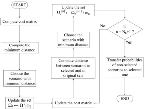
scenarios based on Kantorovich distance, in this paper we have utilized fast forward selection algorithm [9]. This algorithm is a repetitive one, in which an empty scenario tree is formed, then scenarios that minimize Kantorovich distance between initial and selected sets are chosen. When the needed number of scenarios is selected, this algorithm is terminated. Then the probability for each scenario that is not selected is transferred to closest selected scenario. Finally, a reduced scenario tree with de-termined possibility is obtained. Figure 1 shows the flowchart of this selection algorithm.
3. Objective function
As it is mentioned in previous sections, the objective of energy man-agement system of smart microgrid is submitting optimal bids in day-ahead electricity market via maximizing expected profit for smart mi-crogrid operation. Thus in this section, the objective function is defined as maximizing expected profit.
Figure 1. Fast forward selection algorithm
max N S
X
s=1
ρsP rof its (3.1)
subject to:
P rof its=− N T
X
t=1
λdat,sPtda+ (
N T
X
t=1
λdat,sdt,s (3.2)
−
N T
X
t=1 N C
X
c=1 N K
X
k=1
πc,kILt,c,k,s− N T
X
t=1 N DG
X
i=1 Ci,t,sOP E
−
N T
X
t=1
λrealt,s (Pt,sreal)−
N T
X
t=1
λpent P
pen t,s
)
The objective function consists of the revenues from selling electric-ity to the loads and in the electricelectric-ity markets, minus the cost of loads interruption, the power purchasing cost from electricity markets, the microturbines operating cost, and the bids deviation cost. In Eq. (3.2),
P rof its is the earned profit from each scenario s. Each scenario
ex-presses a state from uncertainty set of the given smart microgrid with probability of ρs. The smart microgrid after submitting its bids for
power exchange in day-ahead electricity market Ptda, it will exchange the amount of Preal
t,s = Pt,sdel−Ptda with real time electricity market in
order to compensate for deviation from bid values in previous stage.
Pt,sdel expresses real value of exchanged power with upstream grid in the operating day. If submitted bid values deviate from real values of ex-changed power, the objective function will include penalty ofλpent that is illustrated in the last term of Eq. (3.2) and equals to Eq. (3.3). Also,
λda
t,sandλrealt,s refer to the day-ahead electricity market price and the real
time electricity market price at timetin scenario s, respectively.
Pt,spen= P
del t,s −Ptda
(3.3)
3.1. Constraints on objective function (∀t, s). N DG
X
i=1
Pi,t,s+Pt,sdel+ NB
X
b=1
Pb,t,sD −Pb,t,sC (3.4)
=dt,s− NW
X
w=1
Pw,t,s− NP
X
p=1
Pp,t,s− NC
X
c=1 Pc,t,sIL
Equation (3.4) expresses Kirchhoff law on current (KLC) within smart microgrid. In this equation sum of generated power of dispatchable units (Pi,t,s), amount of real power exchanged with upstream grid (Pt,sdel) and
discharged energy (Pb,t,sD ) at any moment under any scenario and in a couple of steps is equal to sum of total consumed load (dt,s) ,total
interrupted loads (Pc,t,sIL ) and total charged energy (Pb,t,sC ). Also, wind generated power Pw,t,s and solar powerPp,t,s are modeled like negative
load. NDG, NB, NW, NP and NC refer respectively to the number of
dispatchable units, number of batteries, number of wind units, number of photovoltaic units available in the system and number of interruptible loads.
Ci,t,sgen =aiVi,t,s+ ∆T Ni
X
m=1
λi,mPi,m,t,s,∀i (3.5)
Pi,t,s=Pi,m,t,smin Vi,t,s+ ∆T Ni
X
m=1
Pi,m,t,s,∀i (3.6) PiminVi,t,s ≤Pi,t,s≤PimaxVi,t,s,∀i (3.7)
Equation (3.5) expresses the linearized generation cost for unit i at time t in scenario s. Pi,m,t,s expresses amount of generated power in
part m of linearized generation cost function for unit i at time t and in scenarios. The amount of incremental cost at any part of linearized generation cost function for unit iis shown with λi,m. Also the binary
value Vi,t,s expresses the commitment status of unit i during the time
intervalttot+ 1 and in scenario s, 1 expresses the commitment of unit during this time and 0 relates to not commitment during this time. Also, ∆T,ai respectively show length of operation time and generation cost
for unit iat its minimum power (Pimin). T is length of operation time. Equations (3.6) and (3.7) express limitations on generation capacity of units [10].
Ci,t,sstart=kstartoni,t,s,∀i (3.8)
Equation (3.8) corresponds to startup cost of microturbines. The startup factor for microturbines (kstart) is considered as fix. Also,oni,t,s
is a binary variable that expresses startup status for uniti at timet in scenario s, such that 1 refers to startup and 0 refers to not startup of unit.
∆min,c≤ILt,c,k,s ≤∆c,k,∀k= 1, c (3.9)
0≤ILt,c,k,s ≤∆c,k−∆c,k−1,∀1≤k≤NK, c (3.10)
Pt,c,sIL =
NK
X
k=1
ILt,c,k,s,∀c (3.11)
∆min,c≤Pt,c,sIL ≤∆max,c,∀c (3.12)
by interruptible load c at time t in step k and scenario s or ILt,c,k,s
which is constrained within its upper limit ∆c,k and its lower limit ∆c,k.
Constraint (3.10) shows the feasibility of ILt,c,k,s. In this relation NK
is the number of steps for load decrement. Equation (3.11) expresses decreased price interruptible load c that is the sum of accepted offered packages. The constraint (3.12) expresses that the amount of decreased price interruptible load cat any time have to be between minimum and maximum of offered loadc.
0≤Pb,t,sC ≤bCb,t,sPbC; 0≤Pb,t,sD ≤bDb,t,sPbD,∀b (3.13)
SoCb,t+1,s =SoCb,t,s+ ∆T
ηbCPb,t,sC Eb
− P
D b,t,s ηD
b Eb
!
,∀b (3.14)
SoCb,N T,s=SoCb,1; Socminb ≤SoCb,t,s≤SoCbmax,∀b (3.15)
bCb,t,s+bDb,t,s= 1; bb,t,sC , bDb,t,s ∈ {0,1},∀b (3.16)
In constraint (3.13), Pb,t,sC and Pb,t,sD show charging and discharging power for batterybat timetin scenariosthat are limited by maximum and minimum charging and discharging power for battery (PbC andPbD). In this constraint bCb,t,s and bDb,t,s are binary variables for which 1 and 0 respectively show charging and discharging status for battery b at timet in scenario s. Dynamic model for energy exchange in battery is illustrated in constraint (3.14), where,SoCb,t,s shows charging status of
batterybat timetin scenario s. ηC
b andηDb respectively show charging
and discharging efficiency of battery b. Also, Eb is energy capacity for
battery k. In constraint (3.15) SoCb,t,s is limited by maximum battery
statusSoCbmax and minimum battery statusSoCbmin. Constraint (3.16) prevents simultaneous charging and discharging battery b at time t in scenarios[6].
4. Numerical results
In the given microgrid a couple of microturbines with startup cost of 2 dollars and emission cost of 0.001 dollar per kilogram and gener-ation cost according to Eq. (4.1) is considered. Also, the maximum
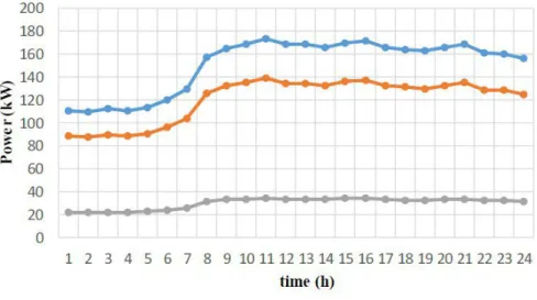
Figure 2. Forecast loads of smart microgrid
generation capacity of microturbines is assumed to be 60 KW. The ca-pacity of battery available in the microgrid is assumed to be 50KWh, also maximum charging and discharging capacity is considered 25KW and the efficiency is assumed 90%. The forecast loads of smart micro-grid is illustrated in Figure2and the forecast price of electricity market is illustrated in Figure 3. The proposed model is solved using CPLEX solver in GAMS.
M icroturbines generation cost= 0.005P2+ 0.03P+ 0.4 (4.1)
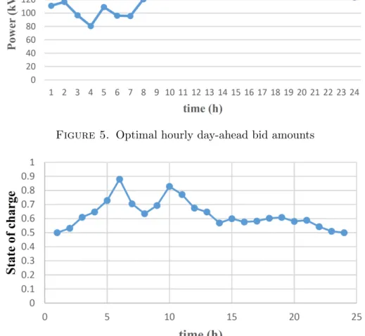
The offered values for interruptible loads for load values of 100,200,400 KW are considered respectively 8,17 and 50 cents per kilowatt. A num-ber of 500 stochastic scenarios for smart microgrid loads, electricity mar-ket price, wind speed and solar irradiance are generated using Monte Carlo method, then these scenarios are reduced to 50 possible scenarios using Kantorovich method as illustrated in Figure 4. Figure 5 shows optimal values for power exchange in day-ahead electricity market (op-timal bids). As it is apparent in the figure smart microgrid purchases
Figure 3. Forecast price of day-ahead electricity market
Figure 4. Reduced stochastic scenarios
power all over the market hours. Also, Figure6shows charging and dis-charging status all over the operation day. As it is shown in the figure during 1 AM to 8 PM when the electricity price is low, the battery is charged and in the high price hours it is discharged.
Figure 5. Optimal hourly day-ahead bid amounts
Figure 6. Expected state of the battery charge over the operating day
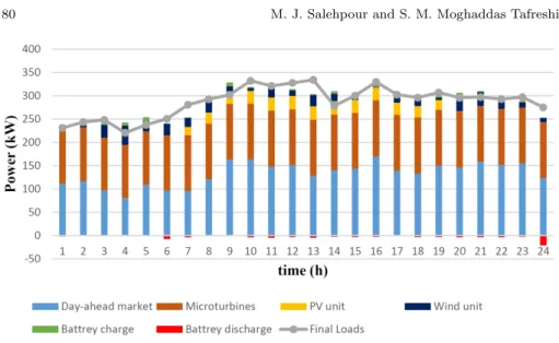
Power balance of smart microgrid including generation of microtur-bines, wind and PV units, charging and discharging battery, exchanging with upstream grid and smart microgrid net load is illustrated in Figure 7. It should be mentioned that optimal value of interruptible load at any hour is 20 KW and this is decreased from total load of smart microgrid and its result is considered in power balance. The expected profitability of smart microgrid is approximated as 403 dollars. Deviation values for
Figure 7. Power balance of smart microgrid components power balance in times of 4,9,14,20 in real time electricity market will be settled during operating day.
5. Conclusions
In this paper profit maximization problem for a smart microgrid via optimal participating in day-ahead electricity market and optimal oper-ation of smart microgrid by two-stage stochastic optimizoper-ation framework is presented. Uncertainties in generation resources (wind and solar), in electrical loads and prices are modeled by generating various scenarios of probabilistic distribution functions corresponding to parameters be-haviors using Monte Carlo method, then in order to reduce calculations time the number of scenarios is reduced using Kantorovich method. The presented model that deals with optimal participation in the electricity market and optimal management of batteries, microturbines and inter-ruptible loads and selling power to various loads leads to maximizing profit.
Acknowledgments
The authors are greatly appreciated the referees for their valuable com-ments and suggestions for improving the paper.
References
[1] J. Shahram and A. Zakariazadeh,Smart distribution systems, Iran University of Science and Technology press,29(2015), 15–30.
[2] P. Agrawal, How ’Micro-grids’ are Poised To Alter The Power Delivery Land-scape, Utility Automation & Engineering T&D,180(2008) 1-10
[3] S. A. Alavi, A. Ahmadian, and M. Aliakbar-Golkar, Optimal probabilistic en-ergy management in a typical micro-grid based-on robust optimization and point estimate method. Energy Conversion and Management,95(2015), 314–325. [4] K. Liu, F. Gao, Z. Wang, X. Guan, Q. Zhai, and J. Wu, Self-balancing robust
scheduling model for demand response considering electricity load uncertainty in enterprise micro-grid, IEEE PES General Meeting — Conference & Exposition (2014).
[5] Y. Xiang, J. Liu, and Y. Liu, Robust Energy Management of Micro-grid With Uncertain Renewable Generation and Load, IEEE Transactions on Smart Grid,
7(2016), 1034–1043.
[6] G. Liu, Y. Xu, and K. Tomsovic,Bidding Strategy for Micro-grid in Day-Ahead Market Based on Hybrid Stochastic/Robust Optimization, IEEE Transactions on Smart Grid,7(2016), 227–237.
[7] S. Nojavan, K. Zare, and M. A. Ashpazi,A hybrid approach based on IGDTMPSO method for optimal bidding strategy of price-taker generation station in day-ahead electricity market, International Journal of Electrical Power & Energy Systems,
69(2015), 335–343.
[8] M. Aien, A. Hajebrahimi, and M. Fotuhi-Firuzabad,A comprehensive review on uncertainty modeling techniques in power system studies, Renewable and Sus-tainable Energy Reviews,57(2016), 1077–1089.
[9] N. Growe-Kuska, H. Heitsch, and W. Romisch,Scenario reduction and scenario tree construction for power management problems, IEEE Bologna Power Tech Conference Proceedings,3(2003), 1–12.
[10] M. Carrion and J. M. Arroyo, A computationally efficient mixed-integer linear formulation for the thermal unit commitment problem, IEEE Transactions on Power Systems,21(2006), 1371–1378.
Mohammad Javad Salehpour
Department of Electrical Engineering, University of Guilan, Rasht, Iran Email: [email protected]
Seyed Masoud Moghaddas Tafreshi
Department of Electrical Engineering, University of Guilan, Rasht, Iran Email: [email protected]