Data processing of remotely sensed airborne
hyperspectral data using the Airborne Processing
Library (APL): Geocorrection algorithm descriptions
and spatial accuracy assessment
Mark A. Warren, Benjamin H. Taylor, Michael G. Grant, Jamie D. Shutler
Plymouth Marine Laboratory, Prospect Place, Plymouth, PL1 3DH. Tel: +44 (0)1752 633432 Fax: +44 (0)1752 633101
Abstract
Remote sensing airborne hyperspectral data are routinely used for appli-cations including algorithm development for satellite sensors, environmental monitoring and atmospheric studies. Single flight lines of airborne hyperspec-tral data are often in the region of tens of gigabytes in size. This means that a single aircraft can collect terabytes of remotely sensed hyperspectral data during a single year. Before these data can be used for scientific analyses, they need to be radiometrically calibrated, synchronised with the aircraft’s position and attitude and then geocorrected. To enable efficient processing of these large datasets the UK Airborne Research and Survey Facility has recently developed a software suite, the Airborne Processing Library (APL), for processing airborne hyperspectral data acquired from the Specim AISA Eagle and Hawk instruments. The APL toolbox allows users to radiometri-cally calibrate, geocorrect, reproject and resample airborne data. Each stage
of the toolbox outputs data in the common Band Interleaved Lines (BIL) format, which allows its integration with other standard remote sensing soft-ware packages. APL was developed to be user-friendly and suitable for use on a workstation PC as well as for the automated processing of the facility; to this end APL can be used under both Windows and Linux environments on a single desktop machine or through a Grid engine. A graphical user in-terface also exists. In this paper we describe the Airborne Processing Library software, its algorithms and approach. We present example results from us-ing APL with an AISA Eagle sensor and we assess its spatial accuracy usus-ing data from multiple flight lines collected during a campaign in 2008 together with in-situ surveyed ground control points.
Keywords: airborne remote sensing, geocorrection, georectification
1. Introduction
1
Remote sensing is an established area of science that can be used to
cap-2
ture information over large, potentially hazardous regions. Earth observation
3
remote sensing is usually performed using systems borne on satellites or
air-4
craft, the first such satellite systems going into orbit in the 1970s. The spatial
5
coverage of earth observation instruments tends to be large (in some cases
6
over 1000 square kilometres (km) per scene), and with an increase in spatial
7
and spectral resolutions the volume of data collected can run into terabytes
8
per instrument per year. This is the case for modern, high resolution
air-9
borne remote sensing instruments, and it is important to be able to process
10
such data volumes in a timely and efficient manner.
11
Aircraft remote sensing is of particular importance for many reasons: it
allows both testing and calibration of expensive satellite systems before they
13
are launched (Baum et al., 2000) and after launch (Magruder et al., 2010);
14
environmental monitoring (Petchey et al., 2011) with rapid deployment
ca-15
pability with high temporal resolution for hazard mapping (Leifer et al.,
16
2012) and as supporting data for other scientific studies (e.g. Neill et al.
17
(2004)). In Europe and North America alone there are many agencies that
18
use airborne remotely sensed data to derive important information about
19
the Earth’s environment. Examples include the US National Oceanic and
20
Atmospheric Administration, NASA, European Space Agency, UK
Environ-21
ment Agency, the UK Natural Environment Research Council (NERC) and
22
the German Aerospace Centre (DLR). Typically these organisations fly with
23
multiple sensors on board, including both passive (such as thermal or
hy-24
perspectral scanning instruments) and active (such as lidar or radar). The
25
large spectral and spatial coverage of airborne remotely sensed data can have
26
many uses including: land classification (Liew et al., 2002), vegetation
iden-27
tification (Cochrane, 2000), habitat monitoring (Kooistra et al., 2008), algal
28
bloom detection (Hunter et al., 2010), mineral identification (Crosta, 1996),
29
pollution monitoring (Horig et al., 2001) and geological mapping (Kruse,
30
1998).
31
The UK NERC Airborne Research and Survey Facility (ARSF) operates
32
an aircraft that collects remotely sensed data which is disseminated for
re-33
search use. Two of the instruments are hyperspectral scanners, the Eagle
34
and Hawk, manufactured by Specim Spectral Imaging Ltd. (Specim, 2012).
35
Data collected from each instrument on a single flight mission can result in
36
very large raw data sets of the order of 200 GB, although on average the size
is 60-80 GB.
38
To accomplish efficient data processing, the Airborne Processing Library
39
(APL) has been developed by the ARSF Data Analysis Node based at
Ply-40
mouth Marine Laboratory (PML). This paper shall discuss the rationale
41
behind APL and how it is exploited within the computing systems at PML
42
including use on a multi-node Grid engine. The processes applied to the
43
hyperspectral data will be introduced and some of the algorithms employed,
44
in particular those for the geocorrection and resampling components, will be
45
discussed in detail. The paper finishes with a look at some example data
46
processing and an analysis on the geocorrection accuracy of a sample data
47
set.
48
2. Airborne Hyperspectral Data Processing
49
Typically, remote sensing data requires two broad stages of pre-processing
50
before it is usable for many topics of research. These are: data
calibra-51
tion (Ahern et al., 1987) and data resampling (Toutin, 2004). To compare
52
information collected by different sensors, by different methods, at
differ-53
ent locations or at different times the data must be calibrated in some way
54
(Ahern et al., 1987). Typically, remotely sensed data should also be
atmo-55
spherically corrected to remove scattering due to atmospheric transmission,
56
making them suitable for direct comparison with ground measurements.
At-57
mospheric correction is outside the scope of this paper and is not performed
58
by the APL software. However, the band interleaved by line (BIL) outputs
59
from APL can be imported into existing software such as the ATCOR4
at-60
mospheric correction package (Richter and Schlapfer, 2002). APL outputs in
BIL rather than band interleaved by pixel (BIP) or band sequential (BSQ)
62
as a performance compromise for further processing, since some data users
63
will want to proceed with spatial processing (where BSQ is better suited)
64
and other spectral processing (where BIP is better suited).
65
Another problem with remotely sensed data is that it may be difficult to
66
analyse without geocorrecting first. For example the captured image is not
67
“North up” or may contain distortions due to platform movements, which
68
can lead to complications when comparing with data from other sources. If
69
this is corrected for, by geocorrecting the data to a well known coordinate
70
system, then it also opens the data up for generation of value-added products.
71
Examples of such being in agriculture and crop management (Seelan et al.,
72
2003) and disaster management (Tralli et al., 2005).
73
2.1. Pre-development of the Airborne Processing Library
74
In 2008 an overhaul of the airborne hyperspectral processing chain was
75
proposed so as to improve data processing efficiency and simplify end user
76
interaction. This was initiated with a review of existing software packages for
77
suitability of automated and user-controlled processing. Packages that were
78
considered included the Specim CaliGeo software (Spectral Imaging Ltd,
79
2004), ENVI software package (Exelis Visual Information Solutions,
Boul-80
der, Colorado), ReSe’s PARGE (Schlapfer and Richter, 2002) software and
81
the Azimuth System UK’s AZ tool package (Azimuth Systems UK, 2005),
82
which in 2008 was the current processing software. No package appeared
83
able to fulfil the requirements of both automated data processing (for
exam-84
ple being able to process multiple flight lines without user interaction) and
85
end-user data processing (i.e. simple to understand, licence-free software
that can be operated with or without a graphical user interface) - with
li-87
censing restrictions for end-users and the inability to freely access the source
88
code being the main disadvantages. The other major disadvantage of the
89
commercial packages is the long term maintenance and security, for example
90
changes in licensing conditions and cost or discontinued support for specific
91
features. Another important factor is transparency, being able to see what
92
is actually being done to the data. Further requirements were being able to
93
react instantly to software bugs and glitches, as well as being able to actively
94
improve and enhance the processing method. With these in mind, having
95
access to source code would be vital for this and played a large factor in the
96
decision to develop APL, which could be tailored for use for both internal,
97
automated processing and end-user data processing.
98
2.2. Airborne Processing Library
99
The Airborne Processing Library was developed with a dual remit; to
100
allow quick and efficient processing of the raw hyperspectral data and as a
101
simple, easy to use toolbox for end-users of the data. To reach these goals it
102
was important that the software adhered to the following points:
103
• Used under Linux operating systems with minimal human interaction
104
• Used under Windows operating systems
105
• Include a graphical user interface (GUI)
106
• Easy to maintain code base
107
To this end APL has been written using standard C++ (with an optional
building as simple as possible. Third party libraries involved are the PROJ4
110
API (PROJ4, 2009) for coordinate re-projections and Blitz++ (Blitz++,
111
2005) for matrix calculations. All executables are built, from the same source
112
directory, using a desktop PC running Linux (Fedora) using the GNU gcc or
113
mingw-gcc compilers (with the code being portable to other compilers). The
114
GUI has been written to operate on Python version 2.7 using the wXpython
115
graphical libraries. The APL software source code is available to download
116
from: https://github.com/arsf/.
117
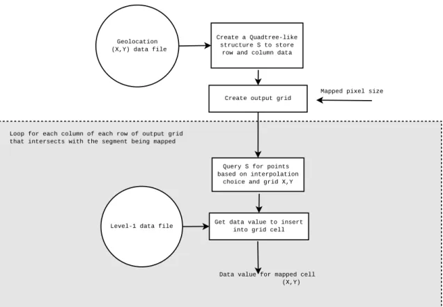
3. Processing Chain
118
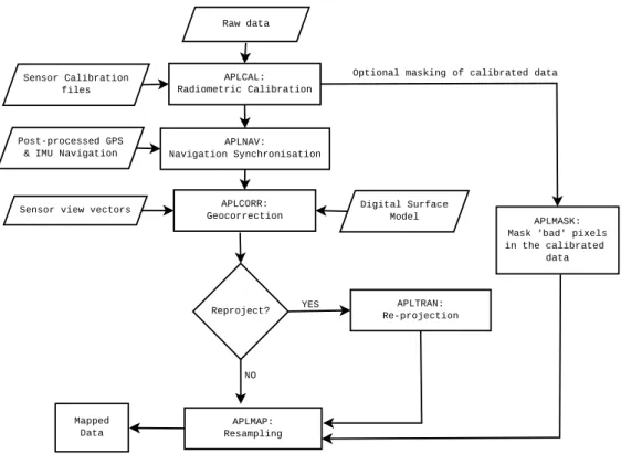
This section describes the data processing chain that employs the APL
119
software. Figure 1 shows a flow diagram of the processing chain including
120
the name of the software utility that performs each action. Details for each
121
action are given in the next sections.
122
[Figure 1 here.]
123
3.1. Prior Information
124
Some information employed in the processing chain exists prior to most
125
data processing and is explained in this section.
126
• Boresight Correction: this is the angular offset between nadir and the
127
true sensor look direction and is estimated at the start of the flying
128
season and each time the sensors are taken out and replaced into the
129
aircraft, using flight lines which have been collected in a suitable
cali-130
bration pattern.
• Instrument Calibration: pre- and post-season the hyperspectral sensors
132
go through a rigorous spectral and radiometric calibration to derive
133
a per-pixel gain file and identify spectral wavelength per band. See
134
Choi (2011) and Taylor et al. (2012) for further details including smear
135
correction, stray light and linearity.
136
• Digital Surface Model (DSM): required to get the best geocorrection
137
accuracy. A DSM is not strictly required as APL will default to an
138
ellipsoid surface, but for hilly and mountainous terrain especially,
pro-139
cessing without a DSM will result in large georeferencing errors.
140
3.2. Radiometric Calibration
141
The raw data need to be calibrated to give meaning to the values and
142
allow comparisons to other data. This procedure starts by normalising the
143
data using “dark” values - data collected with the shutter closed. This
re-144
moves noise due to electrical and system components (Oppelt and Mauser,
145
2007). The data are then scaled using gains calculated during the instrument
146
calibration. A separate mask file is created that contains information on the
147
quality status of each pixel and can be used at a later stage to mask the
148
calibrated data.
149
3.3. Navigation Synchronisation
150
The aircraft GPS position and inertial measurement unit (IMU) attitude
151
are post-processed to get a more accurate and smoother solution. This will
152
usually employ a carrier phase differential GPS method (Hoffman-Wellenhof
153
et al., 2001) using the NovaTel GrafNav software together with Leica IPAS
software to create a blended IMU/GPS solution. This post-processed
naviga-155
tion data must be synchronised to the image data by comparing instrument
156
and GPS time stamps, using spline interpolation to produce per scan line
157
position and attitude estimates.
158
3.4. Masking
159
The optional masking step allows data which have been adversely
af-160
fected during collection or calibration to be masked out (set to zero) so as
161
not to be used in later scientific analyses. These could be pixels that are
162
over-saturated, pixels that have negative values after dark current
subtrac-163
tion, pixels identified as poorly performing during sensor calibration, pixels
164
identified (by eye) as bad during quality checks, pixels affected due to the
165
smear correction of the Eagle sensor or entire missing scan lines.
166
3.5. Georeferencing
167
The georeferencing stage is concerned with computing a per-pixel latitude
168
and longitude map for the image. This is described in detail in section 4.1.
169
3.6. Re-projection
170
The optional re-projection phase of the processing transforms the
lon-171
gitude and latitude data into a specified coordinate system (e.g. Universal
172
Transverse Mercator). This is performed using the open source PROJ4 API
173
library, which currently supports more than 120 projections and 42 ellipsoid
174
models.
3.7. Image Georectification
176
The final stage of the processing is to apply the geocorrection to the
177
radiometrically calibrated data and resample to the desired grid. This is
178
described in detail in section 4.2.
179
3.8. Automated Processing
180
The airborne data processing at PML is performed using the Open Grid
181
Scheduler, where individual jobs are dispatched to particular computing
182
nodes on the network for serial batch processing. Each job is formed of
183
the full chain from radiometric calibration through to image resampling.
Af-184
ter the initial processing directory is set up no user interaction is required
185
during the processing, until the visual quality inspection of the final results.
186
If jobs need to be resubmitted, for example to correct possible timing errors
187
in the navigation synchronisation, then this is a simple task of editing a text
188
configuration file. In practice each job is submitted with a range of timing
189
offsets to apply to the navigation. This means the radiometric calibration
190
need only be performed once with the subsequent processing stages being
191
performed for each time offset.
192
To illustrate the processing overheads and storage requirements, a
re-193
cently collected data set from 2012 consisting of 28 lines (14 of Eagle and
194
14 of Hawk) was processed on the Grid with a single timing offset for each
195
flight line. The mean length of the flight lines processed was 13784 scan
196
lines, which equates to approximately 35 km at a flying speed of 75 metres
197
per second. The raw data amounts to 82 gigabytes (GB) and took a total
198
of 29 hours of processing time to generate 438 GB of processed, resampled
machine is running the Linux (Fedora 17) operating system and has 8 GB of
201
Random Access Memory (RAM) and a Core i3 processor. It should be noted
202
that the PML Grid is in constant use processing various non-related jobs,
203
some of which will take priority over the submitted airborne jobs. A table
204
showing more detailed data can be found in Appendix A. The table shows
205
that there is a wide variation in processing times that is not necessarily linear
206
with increasing line length. Processing two lines, Hawk 8 and Hawk 9, local
207
to a grid node took 23 minutes and 18 minutes respectively, which shows that
208
processing over the PML network can affect processing times by a factor of
209
at least 4 or 5.
210
4. Algorithm details
211
This section describes in detail the algorithms used within APL for the
212
georeferencing and georectification components.
213
4.1. Georeferencing
214
The georeferencing stage is concerned with assigning a latitude and
lon-215
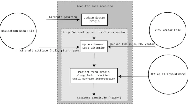
gitude value to each pixel of the image data. The basic algorithm is shown
216
in Figure 2 and is described below.
217
[Figure 2 here.]
218
4.1.1. Input data
219
The input data to the algorithm consists of the synchronised navigation
220
information, a DSM (if available) and information about the image data
221
and sensor configuration, i.e. view vectors. The navigation data file is an
ENVI compatible binary BIL file with one record per image line. Each record
223
contains a time stamp and the sensor position (in WGS-84 latitude, longitude
224
and altitude) and attitude (roll, pitch and yaw). The sensor position is
225
constructed from the aircraft GPS position and the sensor lever arms - the
226
distance between the GPS antenna and the sensor origin. Similarly, the
227
attitude values also contain sensor boresight corrections.
228
The DSM is an elevation model that includes the same area as the scene
229
that is to be geocorrected. It is a binary single band BIL file which
con-230
tains the height values georeferenced to the WGS-84 latitude and longitude
231
geographic projection.
232
The sensor view vector file contains an angular vector describing the
233
sensor look angle from the centre of each pixel of the image capture device.
234
These have been calculated using the focal geometry of the sensor. The file
235
is again a binary BIL file.
236
4.1.2. Algorithm
237
The algorithm follows the general mathematical direct georeferencing
238
model such as described in Muller et al. (2002).
239
After initial parameter setup and checks on the input data, the algorithm
240
works on a per scan line basis starting with the earliest collected line. The
241
aircraft position is converted from longitude, latitude, height (LLH) into an
242
Earth Centred Earth Fixed (ECEF) Cartesian XYZ value. Next the sensor
243
view vectors and aircraft attitude are used to create look vectors in ECEF
244
XYZ with the origin at the aircraft position. This is demonstrated in Figure
245
3.
[Figure 3 here.]
247
If no DSM is used then these view vectors are projected down on to the
248
ellipsoid surface and the intersection point is stored. This is repeated for each
249
sensor look vector of the scan line. Finally, the intersect points are converted
250
to LLH and written out to a BIL file. The algorithm then moves onto the
251
next scan line.
252
If a DSM is available then the surface is read into memory at the start
253
of the algorithm, cropped to an over estimate of the predicted cover of the
254
hyperspectral data in order to reduce memory usage. The
closest-to-nadir-255
looking vector is detected and used as the start point for the scan line
pro-256
cessing, with the processing continuing for each sensor look vector to the
257
starboard of nadir followed by those port of nadir. The aircraft position in
258
(longitude, latitude) is selected as a ‘seed point’ for the intersection algorithm
259
as it is assumed that this is close to the nadir view vector intersection. The
260
three nearest DSM points to the seed position are found and a planar surface
261
created, bounded by the 3 DSM vertices. The intersect point between the
262
ECEF XYZ look vector and planar surface is calculated, using basic vector
263
geometry, and if it is contained within the area defined by the 3 DSM
ver-264
tices then the intersect is stored and the seed point is updated to this new
265
position, ready for the next sensor look vector. If the intersection is outside
266
of the triangle formed by the 3 DSM vertices then 3 new vertices are selected
267
such that they form the opposite triangle which would complete a square.
268
The procedure is repeated and if no intersect is found then the next 3 vertices
269
are selected using a spiral algorithm employed on the seed position such that
270
it is updated as shown in Figure 4. This will be made more efficient in future
by deriving the quadrant containing the intersect point (from the look vector
272
direction) and only checking DSM vertices in that quadrant.
273
The procedure is repeated for each sensor look vector using the updated
274
seed point each time.
275
[Figure 4 here.]
276
4.2. Image georectification
277
The georectification stage is concerned with applying a transformation to
278
the image data and resampling it to a regular grid. The basic algorithm is
279
shown in Figure 5 and is described below.
280
[Figure 5 here.]
281
4.2.1. Inputs
282
The input data required are the outputs from previous stages of the
pro-283
cessing. The image data BIL file that is output by the radiometric calibration
284
or masking stage of APL is required. The geolocation file is also required as
285
this contains the pixel location information. To create the output grid it is
286
also required to have information about the desired pixel resolution. Other
287
inputs may be given depending on how the user wishes the georectified
im-288
age to be created, such as: restricting the output to a particular coverage,
289
selection of image bands to resample, selection of interpolation method to
290
use etc. The output georectified image is an ENVI compatible binary BIL
291
file.
4.2.2. Algorithm
293
The algorithm has three main steps to it, which can be described as:
294
• Restructuring of the input data: to allow efficient searching of the
295
geolocation file
296
• Constructing a Map object: to define the output image and
meth-297
ods to use for the resampling
298
• Creating the resampled image: perform the resampling and write
299
out the resulting image
300
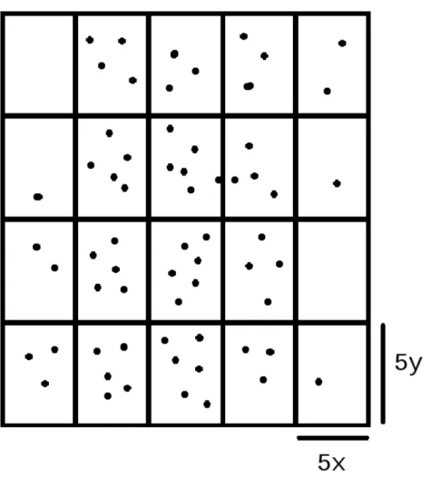
The first step is to take the input geolocation data and construct a
tree-301
like structure (called a treegrid from here on), similar to a quadtree, where
302
each node has fixed dimensions rather than number of ‘children’. This
tree-303
grid groups the points by geographic proximity in order to accelerate
neigh-304
bourhood searches for the interpolation methods. Figures 6 and 7 show the
305
organisation and conceptual model of the treegrid structure. Since the
typ-306
ical amount of image data is large, in some cases >10 GB, it is not feasible
307
to insert the sensor image data into the treegrid as this is stored in RAM.
308
Instead, only the row and column information describing the pixel location
309
within the data file is inserted into the treegrid. From the row and column
310
indices it is possible to identify both the geolocation and the image data
311
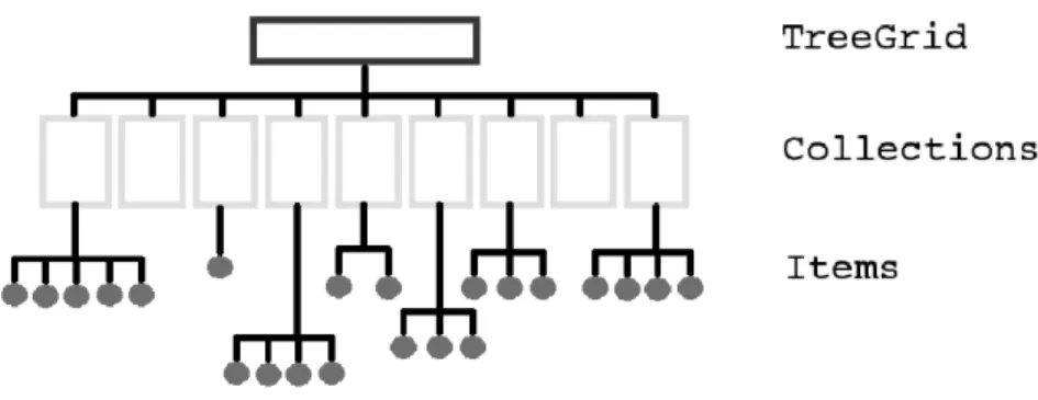
from respective data stores (i.e. files or arrays). Each cell, or node, of the
312
treegrid is known as a ‘collection’, where each collection has the same fixed
313
size in X and Y, defined by a multiple of the average separation of nadir
314
points. A multiplier of 5 is used as this results in a “middle ground” between
315
the efficient searching within the collections and overheads in searching the
treegrid as a whole, with each collection containing approximately 52 items.
317
Therefore, for example, if nadir data points are separated by an average of
318
1 m in the X direction and 2 m in the Y direction, then each collection will
319
have spatial dimensions of 5 m x 10 m.
320
[Figure 6 here.]
321
[Figure 7 here.]
322
The geolocation data file is iterated over and the collection that each pixel
323
belongs to is determined. The information that is inserted into each collection
324
is in the form of an ‘item’ object. Each item contains the corresponding row
325
and column of the geolocation file, identifying a pixel, and a pointer to an
326
‘ItemData’ object, which in turn contains information on where the X, Y
327
geolocation data are stored and methods to read them. When searches are
328
made in the treegrid, all collections within a user-defined radius are searched,
329
to ensure the nearest items are found regardless of which collection contains
330
them.
331
The second step in the algorithm is to construct a ‘Map’ object that
332
defines the grid to output data to. This is the main ‘work horse’ object as it
333
also contains the definitions for interpolating, filling in the grid and writing
334
out the final resampled image. The output grid is constructed based upon
335
the pixel size, the coverage of data (calculated from the tree structure) and
336
the number of bands to output. The Map object also decides how many
337
segments it needs to split the uncorrected image data up into to process
338
efficiently without running low on RAM. By default it allows 1 GB of RAM
for holding image data although this can be increased or decreased as the
340
user wishes.
341
Once this step has completed, the third step of the algorithm is to iterate
342
through each segment in turn, on a row by row basis, and fill the output
343
grid cells with data. By the end of the first segment the full size output
344
file should have been written to disk, zero padded for data yet to be filled
345
in. This allows processing to be done in the order of the uncorrected image
346
data file, irrespective of flight direction or where North is. Further data are
347
inserted on a row by row basis only between the bounds in which the data
348
are contained. For each column of the row to be written, items are found
349
from the tree and passed to the interpolator. The interpolator takes these
350
data and returns the interpolated image value for insertion into the grid. If,
351
however, one of these items contains the ‘masked’ data value for a band being
352
resampled then it is ignored (for that band only) and the next nearest
non-353
masked item is used. If there are none within the search radius then a value
354
of zero is returned from the interpolator for that band. Further information
355
on the interpolation methods can be found in Appendix B.
356
5. Results
357
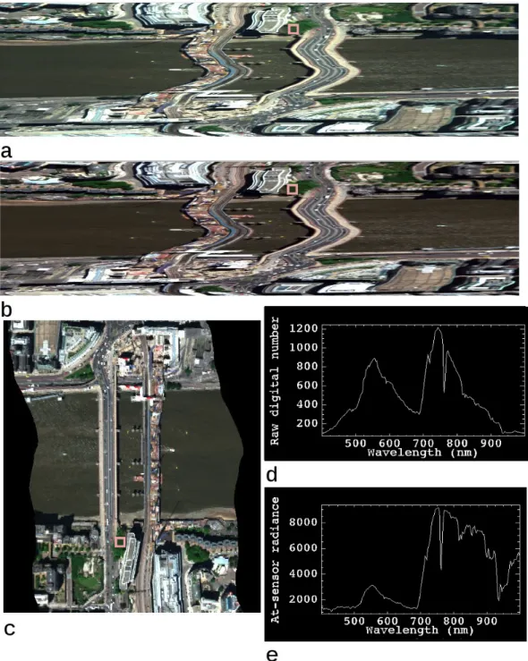
5.1. Data products
358
An example of APL processed Eagle data products, for an area over the
359
River Thames in London, can be seen in Figure 8. The Eagle data shown are
360
(a) prior to applying radiometric calibration, (b) after applying radiometric
361
calibration and (c) shows the data after georectification. Also shown in the
362
figure are two spectral plots from the same green vegetation feature, one
from the raw data and one from the calibrated and georectified data. As no
364
atmospheric correction has been performed on the data, any effects due to
365
the atmosphere will still remain in the data, where these errors will have a
366
direct effect on the amplitude of the reflectance signal but the general shape
367
of the spectra should be unaffected. In Figure 8(e) it can be seen that the
368
calibrated spectra clearly shows the “red edge” at around 700 nano-metres
369
(nm) that one expects to find in vegetation data. In contrast there are two
370
peaks in the raw uncorrected data (Figure 8(d)) illustrating that uncorrected
371
data cannot be relied upon for spectral information.
372
[Figure 8 here.]
373
A second example showing the geocorrection results of APL can be seen
374
in Figure 9. The data in the sensor geometry can be seen at the top in
375
Figure 9(a), and in the main image after georectification into the Ordnance
376
Survey National Grid projection in Figure 9(b). The image background
377
includes Ordnance Survey VectorMap District OpenData to illustrate the
378
geocorrected data. The top left of Figure 9(b) shows a zoomed view to
379
highlight the geocorrection at one of the motorway junctions.
380
[Figure 9 here.]
381
5.2. APLCORR Georeferencing analysis
382
The accuracy of the georeferencing of the data has been tested using
hy-383
perspectral data collected in 2008 over a calibration site in Cambridgeshire,
384
UK. The site contains seven GPS surveyed targets which are visible in the
385
APL and the seven targets were identified from the images prior to
resam-387
pling. The georeferencing output were re-projected into a Universal
Trans-388
verse Mercator projection (Zone 30) for ease of dealing with errors in metres
389
(m) rather than degrees. Not all GPS control points were visible in each
390
dataset. Figure 10 shows the calibration site with the targets identified. The
391
post-processed navigation solution file contains data at 200 Hz, and the
im-392
age data is recorded at 40 frames per second. A digital surface model has
393
been used generated from the NEXTMap 5 m resolution product (Intermap
394
Technologies, 2007).
395
[Figure 10 here.]
396
Appendix C shows the full dataset. The Easting and Northing errors
397
have been converted to along and across track errors by rotation using the
398
mean heading of the aircraft for each section covering the GCPs for each
399
flight line. The mean absolute along track error from the 7 targets and 8
400
flight lines (42 samples in total) for the Eagle sensor is 0.74 m ± 0.58 m.
401
The mean absolute across track error is 0.39 m ± 0.25 m. We expect larger
402
measurement errors in the along track since the spatial resolution is lower in
403
this direction. At nadir the along track pixel separation is approximately 1.9
404
m whereas the across track pixel separation is approximately 0.60 m. This
405
would lead us to expect a higher reported error in the along track direction
406
as the centre of the pixel is being used as the identified location, and this
407
is observed in the results. We can take the ratio of the error versus the
408
pixel separation to approximate the error in terms of pixel size, giving the
409
following mean absolute along track error (at nadir): 0.39 ± 0.31 and across
track error (at nadir): 0.65 ±0.42 reported in pixel size. However, it should
411
be noted that the pixel size will vary along and across track due to the surface
412
topography, aircraft altitude and velocity and target swath position.
413
6. Conclusions
414
The Airborne Processing Library (APL) toolbox has been developed and
415
in operational use since 2011. It allows users to radiometrically calibrate,
416
geocorrect, re-project and re-sample remotely sensed optical airborne data. It
417
can be operated on Windows or Linux systems via command line, a graphical
418
user interface (GUI) or through a Grid Engine. The core geocorrection and
419
resampling algorithms have been discussed. The absolute along and across
420
track spatial geocorrection accuracy have been assessed and reported. The
421
reduced along track accuracy is likely due to the lower spatial resolution
422
(larger spatial coverage) of the sensor configuration in this direction. A high
423
spatial accuracy is important when analysing large volumes of data as it
424
allows much easier dataset integration within Geographic Information System
425
(GIS) applications and other tools used for post-processing and analysing
426
such data.
427
Acknowledgements
428
The authors would like to thank Dr Peter Land for useful discussions on
429
reflectance spectra of ground targets. Figure 9 contains Ordnance Survey
430
OpenData c Crown copyright and database right 2013. The hyperspectral
431
data used in this report were collected by the Natural Environment Research
432
References
434
Ahern, F. J., Brown, R., Cihlar, J., Gauthier, R., Murphy, J., Neville, R. A.,
435
Teillet, P. M., 1987. Radiometric correction of visible and infrared remote
436
sensing data at the Canada Centre for Remote Sensing. International Journal
437
of Remote Sensing 8 (9), 1349–1376.
438
Azimuth Systems UK, 2005. AZGCORR: User’s manual. 57pp URL: http:
439
//arsf.nerc.ac.uk/documents/azgcorr_v5.pdf, [Accessed March 2013].
440
Baum, B. A., Kratz, D. P., Yang, P., Ou, S., Hu, Y., Soulen, P. F., Tsay,
S.-441
C., 2000. Remote sensing of cloud properties using modis airborne simulator
442
imagery during success 1. data and models. Journal of Geophysical Research
443
105 (D9), 11767–11780.
444
Blitz++, 2005. Blitz++ library v0.9. URL: http://sourceforge.net/
445
projects/blitz/, [Accessed January 2013].
446
Catmull, E., Rom, R., 1974. A class of local interpolating splines. In:
Barn-447
hill, R. E., Reisenfeld, R. F. (Eds.), Computer Aided Geometric Design.
448
Academic Press, New York, pp. 317–326.
449
Choi, R. K. Y., 2011. Characterisation of NERC ARSF AISA Eagle and
450
Hawk. In: European Association of Remote Sensing Laboratories (EARSeL)
451
7th SIG-Imaging Spectroscopy Workshop, Edinburgh, 11-13 April. 57pp
452
URL: http://www.earsel2011.com/content/download/Proceedings/S7_
453
6_YoungChoi_pres.pdf, [Accessed October 2013].
454
Cochrane, M. A., 2000. Using vegetation reflectance variability for species
level classification of hyperspectral data. International Journal of Remote
456
Sensing 21 (10), 2075–2087.
457
Crosta, A. P., 1996. High Spectral Resolution Remote Sensing for
Min-458
eral Mapping in the Bodie and Paramount Mining Districts, California. In:
459
International Archives of Photogrammetry and Remote Sensing (IAPRS),
460
Vol.XXXI, ISSN 1682-1750. pp. 161–166.
461
Hoffman-Wellenhof, B., Lichtenegger, H., Collins, J., 2001. GPS: Theory and
462
Practice. Springer-Verlag, 382pp.
463
Horig, B., Kuhn, F., Oschutz, F., Lehmann, F., 2001. Hymap
hyperspec-464
tral remote sensing to detect hydrocarbons. International Journal of Remote
465
Sensing 22 (8), 1413–1422.
466
Hunter, P. D., Tyler, A. N., Carvalho, L., Codd, G. A., Maberly, S. C., 2010.
467
Hyperspectral remote sensing of cyanobacterial pigments as indicators for cell
468
populations and toxins in eutrophic lakes. Remote Sensing of Environment
469
114 (11), 2705–2718.
470
Intermap Technologies, 2007. NEXTMap Britain: Digital terrain mapping of
471
the UK. NERC Earth Observation Data Centre. URL: http://badc.nerc.
472
ac.uk/view/neodc.nerc.ac.uk__ATOM__dataent_11658383444211836,
473
[Accessed October 2013].
474
Kooistra, L., Mucher, S., Niewiadomska, A., 2008. Monitoring of natura
475
2000 sites using hyperspectral remote sensing: Quality assessment of field
476
and airborne data for Ginkelse and Ederheide and Wekeromse Zand. Tech.
Kruse, F. A., 1998. Advances in hyperspectral remote sensing for geologic
479
mapping and exploration. In: Proceedings 9th Australasian Remote Sensing
480
Conference, Sydney, Australia.
481
Leifer, I., Lehr, W. J., Simecek-Beatty, D., Bradley, E., Clark, R., Dennison,
482
P., Hu, Y., Matheson, S., Jones, C. E., Holt, B., Reif, M., Roberts, D. A.,
483
Svejkovsky, J., Swayze, G., Wozencraft, J., 2012. State of the art satellite and
484
airborne marine oil spill remote sensing: Application to the BP Deepwater
485
Horizon oil spill. Remote Sensing of Environment 124, 185–209.
486
Liew, S. C., Chang, C. W., Lim, K. H., 2002. Hyperspectral land cover
clas-487
sification of EO-1 Hyperion data by principal component analysis and pixel
488
unmixing. In: IEEE International Geoscience and Remote Sensing
Sympo-489
sium (IGARSS), 2002. Vol. 6. pp. 3111–3113.
490
Magruder, L., Ricklefs, R., Silverberg, E., Horstman, M., Suleman, M.,
491
Schutz, B., 2010. Icesat geolocation validation using airborne photography.
492
IEEE Transactions on Geoscience and Remote Sensing 48 (6), 2758–2766.
493
Muller, R., Lehner, M., Muller, R., Reinartz, P., Schroeder, M., Vollmer, B.,
494
2002. A program for direct georeferencing of airborne and spaceborne line
495
scanner images. In: International Society for Photogrammetry and Remote
496
Sensing (ISPRS) Proceedings XXXIV Part 1.
497
Neill, S., Copeland, G., Ferrier, G., Folkard, A., 2004. Observations and
498
numerical modelling of a non-buoyant front in the Tay Estuary, Scotland.
499
Estuarine, Coastal and Shelf Science 59 (1), 173–184.
Oppelt, N., Mauser, W., 2007. Airborne Visible / Infrared Imaging
Spec-501
trometer AVIS: Design, Characterization and Calibration. Sensors 7 (9),
502
1934–1953.
503
Petchey, S., Brown, K., Hambidge, C., Porter, K., Rees, S., 2011.
Op-504
erational use of remote sensing for environmental monitoring. Tech. rep.,
505
Natural England/Environment Agency Collaboration, 88pp URL: cdn.
506
environment-agency.gov.uk/geho1211bvqs-e-e.pdf, [Accessed January
507
2013].
508
PROJ4, 2009. Proj.4 - cartographic projections library - version 4.7.1. URL:
509
http://trac.osgeo.org/proj/, [Accessed July 2012].
510
Richter, R., Schlapfer, D., 2002. Geo-atmospheric processing of airborne
511
imaging spectrometry data. part 2: Atmospheric/topographic correction.
In-512
ternational Journal of Remote Sensing 23 (13), 2631–2649.
513
Schlapfer, D., Richter, R., 2002. Geo-atmospheric processing of airborne
514
imaging spectrometry data part 1: Parametric orthorectification.
Interna-515
tional Journal of Remote Sensing 23 (13), 2609–2630.
516
Seelan, S. K., Laguette, S., Casady, G. M., Seielstad, G. A., 2003.
Re-517
mote sensing applications for precision agriculture: A learning community
518
approach. Remote Sensing of Environment 88 (1-2), 157–169.
519
Specim, 2012. Specim - spectral imaging ltd. URL:http://www.specim.fi/,
520
[Accessed July 2012].
521
Spectral Imaging Ltd, 2004. SPECIM CaliGeo 4.0..46 AISA+/AISA Eagle
Taylor, B., Choi, K.-Y., Warren, M., Grant, M., Goy, P., Johnson, J.,
524
Panousis, I., 2012. NERC ARSF hyperspectral instruments: calibration
pro-525
cedures, characteristics and effects. In: Proceedings of the Remote Sensing
526
and Photogrammetry Society (RSPSoc) Conference 2012 - Changing how we
527
view the world.
528
Toutin, T., 2004. Geometric processing of remote sensing images: models,
529
algorithms and methods. International Journal of Remote Sensing 25 (10),
530
1893–1924.
531
Tralli, D. M., Blom, R. G., Zlotnicki, V., Donnellan, A., Evans, D. L., 2005.
532
Satellite remote sensing of earthquake, volcano, flood, landslide and coastal
533
inundation hazards. International Society for Photogrammetry and Remote
534
Sensing (ISPRS) Journal of Photogrammetry and Remote Sensing 59 (4),
535
185–198.
536
Appendix A. Processing performance
537
[Table 1 here.]
538
Appendix B. Interpolation of treegrid data
539
There are currently 4 interpolation methods used in the APL resampling:
540
• Nearest neighbour
541
• Inverse distance weighted
542
• Bi-linear
• Cubic
544
The interpolator takes input from a treegrid search - of which there are
545
two types: ‘nearest points’ or ‘nearest quadrant points’. The difference
be-546
tween the two being that ‘nearest points’ search just returns the nearest N
547
items to the given search point, ordered by distance, whereas ‘nearest
quad-548
rant points’ returns the nearest N points ordered by quadrant centred on
549
the search point. For example, in Eastings and Northings, using a ‘nearest
550
quadrant points’ search for one point, will return four points: one to the
551
North-East, one to the South-East, one to the South-West and one to the
552
North-West of the given search point. This search is used for the bilinear and
553
cubic interpolators. The nearest neighbour and inverse distance weighted
in-554
terpolators use the ‘nearest points’ search. Graphical representations of the
555
interpolation methods are shown in Figure 11.
556
[Figure 11 here.]
557
Appendix B.1. Nearest Neighbour
558
The nearest neighbour interpolator simply takes the image data value
559
from the nearest item to the search point.
560
Appendix B.2. Inverse Distance Weighted
561
The inverse distance weighted method follows the basic Shepard method
562
(Shepard, 1968), defined as:
563
wi =distancei−2/Pdistance−j2
564
f(x) = P
wi∗f(i)
Appendix B.3. Bilinear
567
Bilinear interpolation takes the 4 nearest items (A, B, C and D) to the
568
search point, X, such that the items form a quadrilateral containing the
569
search point (see Figure 12). Using the geolocation information of each item
570
the following formulae can be solved for the scalars U and V:
571
P =A+U ∗(B −A)
572
Q=D+U ∗(C−D)
573
X =P +V ∗(Q−P)
574
[Figure 12 here.]
575
The values of U and V, which are within the range 0-1, are then used to
576
weight the item data values in the interpolation formula:
577
f(X) =f(A)∗(1−V)∗(1−U) +f(B)∗(1−V)∗U+f(D)∗(1−U)∗
578
V +f(C)∗U ∗V
579
wheref(x) is the image data value of cell x.
580
Appendix B.4. Cubic
581
Cubic interpolation uses 16 nearest items such that there are 4 in each
582
quadrant surrounding the centre of the cell. Using a series of 1-dimensional
583
cubic Catmull-Rom splines (Catmull and Rom, 1974) these data are
inter-584
polated. The final result is obtained by interpolating with 4 splines in the X
585
direction followed by 1 spline in the Y direction.
586
Appendix C. Geocorrection analysis results
587
[Table 2 here.]
List of Figures
589
1 Flow diagram of the hyperspectral processing chain. . . 31
590
2 Flow diagram of the APL georeferencing algorithm, where
591
FOV is the sensor field of view. . . 32
592
3 Intersection of view vector to find geolocation of image pixel.
593
Using the position of aircraft p and the sensor view vector v,
594
the intersection point with the surface model can be found.
595
In this example, intersection point a is found when using a
596
DSM whereas intersection point b is found if using the ellipsoid
597
surface model. . . 33
598
4 Spiral updating of seed position (square) in the direction of
599
the arrows. Circles represent the DSM vertices. The
dashed-600
line triangles represent the first planar surface to be tested
601
for each seed position, the dotted-line triangles the ‘opposite’
602
plane that would complete a square. Only the first three sets
603
are shown for clarity, with the triangles numbered in the order
604
of being tested. . . 34
605
5 Flow diagram of the APL georectification algorithm. . . 35
606
6 Tree-like structure shown as a 2-dimensional grid overlaying
607
the data points. Each cell of the grid is a ‘collection’
con-608
taining the data points, known as ‘items’. Each collection has
609
dimensions in X and Y (e.g. Eastings and Northings) equal to
610
five times the mean spacing of data points at nadir. Items are
611
inserted into the collection which bounds the item X,Y
posi-612
tion. This will typically result in 25-30 items per collection at
613
nadir, with fewer items per collection at the edge (the number
614
of items in the diagram have been reduced for simplification). 36
615
7 Organisational overview of the treegrid. The treegrid contains
616
a series of collections (defined by geographic region) which
617
in turn contain items (references to image data points). The
618
organisation of data points in a tree like this allows for efficient
619
searching based on the X,Y position. . . 37
8 Example Eagle sensor (a) raw data, (b) radiometrically
cali-621
brated data and (c) georeferenced and resampled data.
Spec-622
tral plots of green vegetation in raw and calibrated data have
623
been plotted to show differences in these data, and shown in
624
(d) and (e) respectively. This feature is highlighted in (a), (b)
625
and (c) by a pink square. Note ‘red edge’ at 700 nm becomes
626
much more apparent in calibrated data than raw data. . . 38
627
9 Example Eagle data that are (a) prior to geocorrection and (b)
628
after geocorrection and resampling. Also shown are Ordnance
629
Survey OpenData vectors with roads in blue, woodland in
630
green and buildings in purple. Top left of (b) shows a zoom
631
window of the junction to highlight the geocorrection. Eagle
632
data is a spiral flight line collected near the south west of the
633
M25 motorway in 2011. . . 39
634
10 The Monks Wood calibration site Cambridgeshire, UK. The
635
seven surveyed GPS targets are circled and numbered. . . 40
636
11 Illustration of the 4 interpolation methods; the filled circle is
637
the cell point to be interpolated and crosses are treegrid items.
638
a) Nearest neighbour interpolation selects the item nearest to
639
the cell to be interpolated. b) For bi-linear interpolation, the
640
nearest item from each quadrant centred on the cell to be
in-641
terpolated is selected, forming a quadrilateral surrounding the
642
cell. A product of two linear interpolations is performed to
643
determine the interpolated value at the cell. c) Cubic
interpo-644
lation finds the nearest 4 items in each quadrant centred on
645
the cell to be interpolated. These 16 items are then used to
646
form a series of Catmull-Rom splines to interpolate the value
647
at the cell. d) Inverse distance weighted interpolation finds
648
up to the nearest N items within a search radius and takes a
649
weighted average, where the weights are based on the inverse
650
of the distance of each item from the cell to be interpolated. . 41
651
12 The calculation of the position of point X in terms of U and
652
V based on 4 surrounding points. U and V are scalars which
653
are used to weight the data values in the bilinear interpolation
654
algorithm. . . 42
Figure 2: Flow diagram of the APL georeferencing algorithm, where FOV is the sensor field of view.
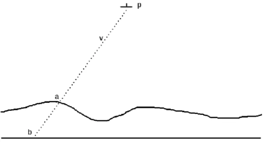
Figure 3: Intersection of view vector to find geolocation of image pixel. Using the position of aircraft p and the sensor view vector v, the intersection point with the surface model can be found. In this example, intersection point a is found when using a DSM whereas intersection point b is found if using the ellipsoid surface model.
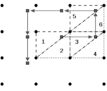
Figure 4: Spiral updating of seed position (square) in the direction of the arrows. Circles represent the DSM vertices. The dashed-line triangles represent the first planar surface to be tested for each seed position, the dotted-line triangles the ‘opposite’ plane that would complete a square. Only the first three sets are shown for clarity, with the triangles numbered in the order of being tested.
Figure 6: Tree-like structure shown as a 2-dimensional grid overlaying the data points. Each cell of the grid is a ‘collection’ containing the data points, known as ‘items’. Each collection has dimensions in X and Y (e.g. Eastings and Northings) equal to five times the mean spacing of data points at nadir. Items are inserted into the collection which bounds the item X,Y position. This will typically result in 25-30 items per collection at nadir, with fewer items per collection at the edge (the number of items in the diagram have been reduced for simplification).
Figure 7: Organisational overview of the treegrid. The treegrid contains a series of collec-tions (defined by geographic region) which in turn contain items (references to image data points). The organisation of data points in a tree like this allows for efficient searching based on the X,Y position.
Figure 8: Example Eagle sensor (a) raw data, (b) radiometrically calibrated data and (c) georeferenced and resampled data. Spectral plots of green vegetation in raw and calibrated data have been plotted to show differences in these data, and shown in (d) and
Figure 9: Example Eagle data that are (a) prior to geocorrection and (b) after geocorrec-tion and resampling. Also shown are Ordnance Survey OpenData vectors with roads in blue, woodland in green and buildings in purple. Top left of (b) shows a zoom window of the junction to highlight the geocorrection. Eagle data is a spiral flight line collected near the south west of the M25 motorway in 2011.
Figure 10: The Monks Wood calibration site Cambridgeshire, UK. The seven surveyed GPS targets are circled and numbered.
Figure 11: Illustration of the 4 interpolation methods; the filled circle is the cell point to be interpolated and crosses are treegrid items. a) Nearest neighbour interpolation selects the item nearest to the cell to be interpolated. b) For bi-linear interpolation, the nearest item from each quadrant centred on the cell to be interpolated is selected, forming a quadrilateral surrounding the cell. A product of two linear interpolations is performed to determine the interpolated value at the cell. c) Cubic interpolation finds the nearest 4 items in each quadrant centred on the cell to be interpolated. These 16 items are then used to form a series of Catmull-Rom splines to interpolate the value at the cell. d) Inverse distance weighted interpolation finds up to the nearest N items within a search radius and takes a weighted average, where the weights are based on the inverse of the distance of each item from the cell to be interpolated.
Figure 12: The calculation of the position of point X in terms of U and V based on 4 surrounding points. U and V are scalars which are used to weight the data values in the bilinear interpolation algorithm.
List of Tables
656
1 Table showing processing performance statistics for processing
657
on the Grid. . . 44
658
2 Absolute errors (in metres) between GPS and target
identifi-659
cation from geocorrection data (prior to resampling). Errors
660
reported in Eastings, Northings and converted to along track,
661
across track. . . 45
Line Process time (hh:mm:ss) Flight length (scan lines) Number of bands
Eagle -1 00:26:32 16245 126
Eagle -2 00:01:18 1881 126
Eagle -3 01:47:31 15321 126
Eagle -4 00:32:42 18098 126
Eagle -5 02:58:43 15646 126
Eagle -6 01:18:35 16868 126
Eagle -7 01:15:55 16153 126
Eagle -8 01:09:05 15693 126
Eagle -9 00:46:33 13492 126
Eagle -10 00:56:02 14219 126
Eagle -11 00:50:24 12323 126
Eagle -12 00:29:54 12047 126
Eagle -13 00:34:06 8643 126
Eagle -14 00:25:03 6909 126
Hawk -1 01:32:31 16247 233
Hawk -2 01:31:23 16539 233
Hawk -3 01:25:32 15322 233
Hawk -4 01:23:33 18099 233
Hawk -5 01:22:43 15646 233
Hawk -6 01:24:46 16868 233
Hawk -7 01:24:14 16155 233
Hawk -8 02:00:16 15694 233
Hawk -9 01:08:51 13492 233
Hawk -10 00:50:58 14221 233
Hawk -11 00:21:39 12324 233
Hawk -12 00:27:45 12049 233
Hawk -13 00:08:17 8645 233
Hawk -14 00:05:23 6910 233
Flight line Target Abs E Abs N Abs Along Abs Across 1 3 0.098 0.334 0.302 0.174 1 4 0.265 0.710 0.682 0.331 1 5 0.467 0.790 0.883 0.249 1 6 0.105 0.436 0.225 0.388 2 3 0.392 0.404 0.439 0.353 2 4 0.465 0.730 0.684 0.531 2 5 0.727 0.400 0.439 0.687 2 6 0.205 1.264 1.278 0.087 2 7 0.355 0.404 0.369 0.391 3 1 1.310 1.765 2.166 0.373 3 2 0.109 0.437 0.223 0.391 3 3 0.558 0.464 0.083 0.721 3 4 0.615 0.170 0.562 0.302 3 5 1.633 1.220 2.024 0.245 3 6 1.375 0.726 1.496 0.424 3 7 1.025 1.456 1.747 0.346 4 1 0.750 0.885 0.764 0.873 4 2 1.621 0.653 1.631 0.627 4 3 0.422 0.576 0.431 0.569 4 4 0.875 0.430 0.882 0.416 4 5 0.197 0.570 0.206 0.567 4 6 0.005 0.546 0.004 0.546 5 3 0.568 1.286 0.534 1.301 5 4 0.395 0.030 0.396 0.020 5 5 2.093 0.270 2.099 0.215 5 6 1.335 0.016 1.334 0.051 6 1 0.250 0.935 0.795 0.552 6 2 0.441 0.017 0.347 0.272 6 3 0.278 0.424 0.062 0.503 6 4 0.045 0.060 0.004 0.075 6 5 0.997 0.150 0.858 0.530 6 6 0.205 0.114 0.230 0.046 6 7 1.105 0.076 0.794 0.772 7 3 0.352 0.936 0.950 0.313 7 4 0.055 0.370 0.323 0.189 7 5 0.183 0.410 0.434 0.115 7 6 0.395 0.264 0.453 0.142 8 3 0.038 1.076 1.071 0.106 8 4 0.385 0.430 0.454 0.357 8 5 0.343 0.180 0.201 0.331 8 6 0.285 0.974 0.990 0.223 8 7 0.445 1.206 1.175 0.521 Mean 0.566 0.586 0.739 0.386 St Dev 0.499 0.429 0.579 0.254