Sharif University of Technology
Scientia IranicaTransactions E: Industrial Engineering www.scientiairanica.com
Multidimensional knapsack problem based on uncertain
measure
L. Cheng
a, C. Rao
a;band L. Chen
c,a,1;a. College of Mathematics and Physics, Huanggang Normal University, Hubei 438000, China. b. School of Science, Wuhan University of Technology, Wuhan 430070, China.
c. College of Mathematics and Sciences, Shanghai Normal University, Shanghai 200234, China. Received 29 August 2015; received in revised form 6 June 2016; accepted 5 September 2016
KEYWORDS Multidimensional knapsack problem; Uncertain network optimization; Uncertain measure; Discount constraint.
Abstract. The researchers of classical multidimensional knapsack problem have always assumed that the weights, values, and capacities are constant values. However, in the real-life industrial engineering applications, the multidimensional knapsack problem often comes with uncertainty about a lack of information about these parameters. This paper investigates a constrained multidimensional knapsack problem under uncertain environment, in which the relevant parameters are assumed to be uncertain variables. Within the framework of uncertainty theory, two types of uncertain programming models with discount constraints are constructed for the problem with dierent decision criteria, including the expected value criterion and the critical value criterion. Taking full advantage of the operational law for uncertain variables, the proposed models can be transformed into their corresponding deterministic models. After theoretically investigating the properties of the models, we do some numerical experiments. The numerical results illustrate that the proposed models are feasible and ecient for solving the constrained multidimensional knapsack problem with uncertain parameters.
© 2017 Sharif University of Technology. All rights reserved.
1. Introduction
The Multidimensional Knapsack Problem (MKP) is one of the most extensively-studied problems in net-work optimization. The task of MKP is to choose a subset of items in which the total value is maximized while the weight does not exceed the specied capacity of each dimension. MKP oers many practical appli-cations in industrial engineering, such as production planning [1], project scheduling [2], service center location [3], and supply chain management [4], etc.
1. Present address: College of Management and Economics, Tianjin University, Tianjin 300072, China.
*. Corresponding author.
E-mail address: [email protected] (L. Chen) doi: 10.24200/sci.2017.4485
For more comprehensive development of MKP, please consult Freville [5]. Due to its wide range of applicabil-ity, the multidimensional knapsack problem was widely studied in deterministic environment. However, in practice, some indeterminacy factors might appear in the problems due to the lack of history data, insucient information, or some other reasons. As previous studies [6,7] pointed out, the available capacity or weight might be unknown due to delay in previous jobs, or the item rewards might depend on market uctuations. Thus, it is not suitable to use the classical models to investigate the multidimensional knapsack problem in these situations.
Several researchers deemed that such indeter-minacy behaves like randomness. Based on this as-sumption, a lot of studies have been investigated within the framework of probability theory. For in-stance, Kosuch [8] studied a two-stage stochastic
knapsack problem with random weights. Feng and Hartman [9] investigated a stochastic knapsack prob-lem with homogeneous-sized items and postponement options. Han et al. [10] considered a certain class of chance-constrained knapsack problems where each item has an independent normally-distributed random weight. For more research on the stochastic knapsack problem, see Kleywegt and Papastavrou [7], Gibson et al. [11], Merzifonluoglu et al. [12], and others.
It is undeniable that probability theory is a useful tool to deal with indeterminacy factors. However, as is known to all of us, a fundamental premise of applying probability theory is that the estimated probability distribution is close enough to the true frequency. Thus, we have to rely on a great quantity of histor-ical data and employ statistics to get the probability distribution. In the real-world, however, there exist many uncertain factors which cannot be ignored when the decision-makers make their decisions. Motivated by this consideration, several researchers have employed fuzzy set theory to deal with nondeterministic param-eters for multidimensional knapsack problem. Okada and Gen [13] proposed the multiple-choice knapsack problems under fuzzy environment. Changdar et al. [14] considered an improved genetic algorithm to solve constrained knapsack problem with fuzzy param-eters. Changdar et al. [15] investigated the knapsack problem with imprecise weight using genetic algo-rithms. Chen [16] proposed a parametric programming approach to analyze the fuzzy maximum total return in the continuous knapsack problem with fuzzy objective weights. Baykasoglu and Ozsoydan [17] developed re-y algorithm to solve dre-ynamic multidimensional knap-sack problems. Kasperski and Kulej [18] considered the knapsack problem with imprecise prots and imprecise weights of items. Our paper diers from those of Okada and Gen [13] and Kasperski and Kulej [18] in the follow-ing aspects. First, we use an uncertain measure, which is a self-dual measure, to describe belief degree of the relevant parameter in the multidimensional knapsack problem. Based on this measure, the operational law in the uncertainty theory is simpler and easier than its counterpart in the fuzzy set theory. The details of operational law of uncertain variable are shown in Section 3. Second, we consider the multidimensional knapsack problem with a price-discount constraint. This type of multidimensional knapsack problem is commonly used in the fruit and/or vegetable retailing systems. Motivated by this discount strategy, our paper establishes a medium between the existing uncer-tainty theory and multidimensional knapsack problem. However, if the uncertain factor comes from the decision-maker's empirical estimation, then it is not suitable to employ random variable or fuzzy variable to describe this kind of uncertain factor. In such cases, we have to invite some domain experts to give the
belief degrees of the weights, values, and capacities. According to Kahneman and Tversky [19], human beings usually overweight unlikely events, thus the belief degree based on experts' estimations may be far from the cumulative frequency. One the one hand, in 2012, Liu [20] pointed out that if we insist on dealing with the belief degree by using probability theory in this situation, some counter-intuitive phenomena might occur. On the other hand, the fuzzy set theory is not self-consistent in mathematics and may lead to several counter-intuitive paradoxes in practice [21]. The details of counterintuitive paradoxes will be given in Section 2. Therefore, in this situation, we have no choice but to use the uncertainty theory, founded by Liu [22], to deal with the belief degree in the multidimensional knapsack problems.
Although multidimensional knapsack problems have been widely investigated, it has not been studied within the framework of uncertainty theory. This is because the uncertainty theory is a quite recent and new tool to deal with the belief degree mathematically. To the best of our knowledge, only Peng and Zhang [23] analyzed the uncertain knapsack problem with single-capacity constraint. Following the main literature in the eld of uncertainty theory, in their paper [23], the values and the weights were characterized as uncer-tain variables. But, in the real-life decision-making problems, the decision-makers usually encounter the situations of the knapsack problem with multiple-capacity constraints. Since no one has investigated the multidimensional knapsack problem under uncertain environment before, we have made attempts to ll this gap. Specically, this paper considers a constrained multidimensional knapsack problem, which is usually encountered in the fruit and/or vegetable retailing systems based on uncertain measure. We employed two kinds of uncertain variables, i.e. linear uncertain and zigzag uncertain variables, to characterize the weights, values, and capacities of the multidimensional knapsack problem with a discount constraint. Within the framework of uncertainty theory, two types of uncertain programming models are constructed for the problem with dierent criteria, e.g. the expected value and the critical value criteria. Based on the operational law for uncertain variables, some theoretical analyses are provided. The theoretical results illustrate that the maximum value of chance-constrained programming model actually decrease with respect to the predeter-mined condence level.
The structure of this paper is as follows. In Section 2, we state the fact that the fuzzy set theory cannot be employed to model the imprecise parameters in multidimensional knapsack problem. To facilitate the understanding of the paper, some basic concepts and results related to uncertainty theory are outlined and the classical multidimensional knapsack problem is
briey reviewed in Section 3. Section 4 proposes two types of uncertain programming models for uncertain multidimensional knapsack problem and transforms the models into their corresponding deterministic forms within the framework of uncertainty theory. Some numerical examples are given to show the applications of the proposed models in Section 5. Section 6 gives some concluding remarks and possible directions for the future work.
2. Why using uncertain measure?
In this section, we present the fact that the fuzzy set theory cannot be employed to model the imprecise weights, imprecise values, and imprecise capacities in multidimensional knapsack problem under uncertain environment.
As discussed in the introduction, the previous studies of using the fuzzy set theory to investigate the multidimensional knapsack problem have indeed opened a new research perspective for solving multi-dimensional knapsack problems with imprecise param-eters given by experts' estimations. However, with a deeper research on the problem, we nd out that several counterintuitive paradoxes will appear if fuzzy variables are employed to characterize the imprecise parameters of MKP.
We take the imprecise capacities of MKP as an example to illustrate several counterintuitive paradoxes when we use the fuzzy set theory to study the mul-tidimensional knapsack problem. Supposing that the capacity of the dierent knapsack is regarded as a fuzzy number, we have a membership function to describe it. In the fuzzy set theory, possibility measure (Pos) and necessity measure (Nec) are the two basic measures. Assume that the membership function of knapsack capacity is a triangular fuzzy variable, (8; 9; 10). Then, we can obtain the following two paradoxes. First, based on the membership function, it is known from possibility theory that Posf = 9g = Posf 6= 9g and Necf = 9g = Necf 6= 9g. In other words, the capacity of knapsack, being exactly 9 and not exactly 9, has the same belief degree in possibility measure and necessity measure. This implies that the two events will happen equally likely. This conclusion is obviously unreasonable. Second, the capacity of knapsack is exactly 9 with belief degree 1 in possibility measure. However, this conclusion is also hard to accept because the belief degree of exactly 9 should be almost zero.
It can be seen from the above two counterintuitive examples that the fuzzy set theory is not a suitable tool to model the imprecise weights, imprecise values, and imprecise capacities in multidimensional knapsack problem when the relevant parameters are given by experts' estimations. In order to handle this diculty, Liu [22] introduced an uncertain measure within the
framework of uncertainty theory. When we use the uncertain measure to gauge the subjective uncertain quantities, the abovementioned paradoxes will disap-pear immediately. In fact, the uncertainty theory has been widely applied to various real-life industrial engineering problems, e.g. knapsack problem with sin-gle capacity [23], optimal assignment problem [24], the shortest path problem [25], railway transportation planning problem [26], supply chain contract design problem [27], and so on. In the next section, we will introduce the uncertainty theory briey.
3. Preliminary
In this section, some basic concepts and results of uncertainty theory are recalled, and the classical mul-tidimensional knapsack problem is briey reviewed. 3.1. Uncertainty theory
Uncertainty theory was founded by Liu [22] in 2007 and rened by Liu [21] in 2010. The uncertain pro-gramming, established by Liu [28], was a type of math-ematical programming involving uncertain variables. In recent years, several scholars have employed uncer-tain programming to investigate the real-life decision-making problems. For instance, Gao [25] studied the uncertainty distribution of the shortest path length and proposed an eective method to nd the -shortest path and the shortest path in an uncertain network. Zhang and Peng [24] employed uncertain programming to deal with uncertain optimal assignment problem in which prot is an uncertain variable. Recently, Peng et al. [29] presented a state-of-the-art review on the recent advances in the area of uncertain network optimization. Assume that is a nonempty set, and L is a -algebra over . Each element in L is called an event. A set function M:L ! [0; 1] is called an uncertain measure if it satises the following three axioms [22]: Axiom 1 (normality axiom). Mf g = 1 for the universal set ;
Axiom 2 (duality axiom). Mfg + Mfcg = 1 for
any event 2 L;
Axiom 3 (subadditivity axiom). For every count-able sequence of events 1; 2; , we have:
M (1
[
i=1
i
)
1
X
i=1
Mfig:
Denition 1 [22]. Let be a nonempty set, L a -algebra over , and M an uncertain measure. Then, the triplet ( ; L; M) is called an uncertainty space.
Product uncertain measure M on product -algebra L was dened by Liu [30], thus producing the following product axiom.
Axiom 4 (product axiom). Let ( k; Lk; Mk) be
uncertainty spaces for k = 1; 2; The product uncer-tain measure, M, is an unceruncer-tain measure satisfying:
M (1
Y
k=1
k
) = ^1
k=1
Mkfkg;
where k refers to arbitrarily chosen events from Lk
for k = 1; 2; , respectively.
Uncertain variable is mainly used to model the uncertain quantities. A formal denition was given by Liu [22] as follows:
Denition 2 [22]. An uncertain variable is a func-tion from an uncertainty space ( ; L; M) to the set of real numbers such that f 2 Bg is an event for any Borel set B.
On the basis of uncertain measure, Liu [22] gave the denition of uncertainty distribution of an uncer-tain variable, , which was dened by (x) = Mf xg. If an uncertainty distribution, (x), is a continuous and strictly increasing function with respect to x at which 0 < (x) < 1 and the following limitations hold:
lim
x! 1(x) = 0; x!+1lim (x) = 1;
then, uncertainty distribution, (x), is said to be regular [21].
Denition 3 [30]. Uncertain variables 1; 2; ; n
are said to be independent if:
M ( n
\
i=1
(i2 Bi)
) = ^n
i=1
Mfi2 Big;
for any Borel sets B1; B2; ; Bn.
Theorem 1 [21]. Let 1; 2; ; n be independent
uncertain variables with regular uncertainty distribu-tions 1; 2; ; n, respectively. If function f(x1;
; xm; xm+1; ; xn) is strictly increasing with
re-spect to x1; x2; ; xm and strictly decreasing with
respect to xm+1; xm+2; ; xn, then the uncertain
vari-able:
= f(1; ; m; m+1; ; n);
has an inverse uncertainty distribution:
1() = f( 1
1 (); ; m1(); m+11 (1 );
; 1
n (1 )):
Theorem 2 [21]. Let 1; 2; ; n be independent
uncertain variables with regular uncertainty distribu-tions 1; 2; ; n, respectively. If function f(x1;
; xm; xm+1; ; xn) is strictly increasing with
re-spect to x1; x2; ; xm and strictly decreasing with
respect to xm+1; xm+2; ; xn, then:
Mff(1; ; m; m+1; ; n) 0g
if and only if: f( 1
1 (); ; m1(); m+11 (1 ); ;
1
n (1 )) 0:
According to Theorems 1 and 2, we can easily ob-tain the inverse uncerob-tainty distribution of function f(1; 2; ; n). Therefore, we can transform an
indeterminacy model into a deterministic form based on Theorems 1 and 2. On the basis of uncertain mea-sure, Liu [22] dened the expected value of uncertain variables as follows. If be an uncertain variable, then the expected value of is dened by:
E[] = Z +1
0 Mf rgdr
Z 0
1Mf rgdr;
provided that at least one of the integrals was nite. If had an uncertainty distribution, (x), Liu [22] veried that the expected value could be calculated by:
E[] = Z +1
0 (1 (x))dx
Z 0
1(x)dx:
In addition, Liu [21] veried that if the uncertainty dis-tribution, (x), was regular, then E[] =R01 1()d.
Theorem 3 [21]. Assume that 1 and 2 are
indepen-dent uncertain variables with the nite expected values. For any real numbers, a1 and a2, we have:
E[a11+ a22] = a1E[1] + a2E[2]:
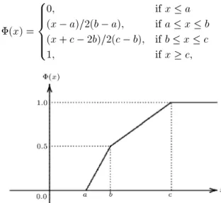
Example 1. Uncertain variable, , is called zigzag if it has a zigzag uncertainty distribution (see Figure 1):
(x) = 8 > > > < > > > :
0; if x a (x a)=2(b a); if a x b (x + c 2b)=2(c b); if b x c 1; if x c;
Figure 2. Linear uncertainty distribution.
denoted by Z(a; b; c); where a, b, and c are real numbers with a < b < c. The inverse uncertainty distribution, 1(), of uncertain variable, , is given by:
1() =
(
(1 2)a + 2b; if < 0:5 (2 2)b + (2 1)c; if 0:5 The expected value of is E[] = (a + 2b + c)=4. Example 2. Assume that L(a; b) is a linear uncertain variable, where a and b are real numbers with a < b. Its uncertainty distribution, (x), (see Figure 2) and inverse uncertainty distribution, 1(), are given
by:
(x) = 8 > < > :
0; if x a (x a)=(b a); if a x b 1; if x b; and:
1() = (1 )a + b;
respectively. The expected value of is E[] = (a+b)=2. 3.2. Classical multidimensional knapsack
problem with discount constraint
In this section, we present the formulation of Multi-dimensional Knapsack Problem (MKP) with discount constraint in deterministic environment. Generally speaking, MKP is concerned with a set of items, N = f1; 2; ; ng, to be packed in a knapsack that has a set of dimensions, M = f1; 2; ; mg. The maximum capacity of each dimension, i, is denoted as ci, i = 1; 2; ; m. Each item, j 2 N, has a weight,
wij, in each dimension, and a corresponding value vj,
i = 1; 2; ; m, j = 1; 2; ; n. The task of MKP is to choose a subset of items that the total value is maximized, while the weight does not exceed specied capacity, ci, of each dimension, i. Motivated by various
examples in the real-life decision making problems, we consider the MKP with discount constraint. For example, some of the objects are available to which
discount has been oered if the selected quantity is greater than a predetermined level. The fruit and/or vegetable retailing systems exhibit the characteristic where the wholesalers adopt the discount strategy. If the minimum predetermined amount of object is selected, then a discount is to be considered for that item and the total discount must reach or exceed a predetermined total discount, D. For jth item, if minimum, mj, unit of object is consumed, the discount
is dj; otherwise, no discount is considered and the total
predetermined minimum discount is D. Therefore, we construct the mathematical model for multidimen-sional knapsack problem with discount constraint as follows:
maxXn
j=1
vjxj;
subject to:
n
X
j=1
wijxj ci; for i = 1; 2; ; m;
n
X
j=1
djyj D;
xj2 f0; 1g; yj2 f0; 1g; for j = 1; 2; ; n: (1)
It is necessary to point out that the rst constraint requires that the knapsacks not exceed the capacity of any knapsack. The second constraint is the discount constraint. Variables xj and yj are all binary
vari-ables. The detailed characteristics of these two binary variables are as follows. If the jth item is selected, then xj = 1; otherwise xj = 0. If xj mj (mj take value
from [0; 1]) and dj> 0, then yj = 1; otherwise yj= 0.
4. Uncertain multidimensional knapsack models
Model (1) assumes that the weights, values, and capac-ities are constant values. However, in practice, these parameters are not usually constant values. As dis-cussed in the introduction, we always lack history data, or even history data are invalid. Then, one problem is naturally produced; that is, how can we deal with this kind of indeterminacy factor in the multidimensional knapsack problem? In this situation, the relevant data can only be obtained from the decision-makers' empirical estimations in a practical way. As mentioned before, the uncertainty theory provides a new tool to deal with uncertain information, especially subjective or empirical information. Hence, in this paper, we assume that each item, j, has an uncertain weight, ij, in each dimension and an uncertain value, j; each
capacity of any knapsack is an uncertain variable, i,
and the discount of the jth item is also an uncertain variable j, i = 1; 2; ; m, j = 1; 2; ; n.
Without loss of generality, we also assume that the parameters are nonnegative and independent un-certain variables. Such an independent assumption is extensively used in a recent work in the area of uncertain network optimization (Gao [25], Zhang and Peng [24], and Peng et al. [29], to name a few). For the sake of convenience, all the uncertain values, uncertain weights, uncertain capacities, and uncertain discount coecients are presented by un-certain vectors = (1; 2; ; n), = (ijji =
1; 2; ; m; j = 1; 2; ; n), = (1; 2; ; m) and
= (1; 2; ; n), respectively. Then, the uncertain
multidimensional knapsack can be denoted by K = (V; ; ; ; ) in which V is the maximum value by which the knapsack can be carried out. Then, the total value of maximum pack scheme of uncertain multidimensional knapsack is f() =Pnj=1jxj:
It is clear that f() is also an uncertain variable because uncertain values j are all uncertain variables
for j = 1; 2; ; n. Then, the Uncertain Multidimen-sional Knapsack Problem (UMKP) can be expressed as follows:
max
n
X
j=1
jxj
subject to:
n
X
j=1
ijxj i 0; for i = 1; 2; ; m;
n
X
j=1
jyj D;
xj 2 f0; 1g; yj 2 f0; 1g; for j = 1; 2; ; n. (2)
Model (2) turns meaningless in the sense of mathemat-ical viewpoints under uncertain environment. In order to optimize the objective, it is inevitable for us to rank uncertain variables according to some decision criteria. Generally speaking, there exist two kinds of decision criteria to rank the uncertain variables according to the manager's philosophy of modeling uncertainty. The two kinds of decision criteria are the expected value criterion and the critical value criterion which are based on the manager's dierent risk attitude. On the one hand, the main idea of the expected value criterion is to optimize the expected value of the manager's objective. On the other hand, the essential idea of the critical value criterion is to optimize the critical value of the manager's objective with predetermined condence level. In the next section, we will employ these
two kinds of criteria to rank the uncertain variables and construct two kinds of uncertain programming models with discount constraint. One is the expected value model, and another is the chance-constrained programming model.
4.1. Expected value model
Dierent from a deterministic environment, the total value for UMKP is an uncertain variable under uncer-tain environment. It is dicult for us to rank two un-certain variables directly. The rst way is to adopt the expected value criterion to rank the uncertain variable. Therefore, the rst type of uncertain programming, i.e. the so-called expected value model, is constructed based on this kind of ranking criterion. The main idea of the expected value model is to optimize the expected value of objective function subject to some expected constraints. Motivated by this most understandable method for modeling the real-life industrial engineering problems, we present the expected value model for UMKP as follows:
max E 2 4Xn
j=1
jxj
3 5 ; subject to:
E 2 4Xn
j=1
ijxj i 0
3
5 ; for i = 1; 2; ; m; E
2 4Xn
j=1
jyj
3 5 D;
xj 2 f0; 1g; yj 2 f0; 1g; for j = 1; 2; ; n: (3)
We can see that Model (3) is constructed under the light of uncertain environment. To seek the optimal solution of Model (3), it is necessary for us to compute expected values of the relevant parameters. In order to solve the model easily, it is better for us to convert the model into its crisp equivalent model. Taking full advantage of the concept of expected value for uncertain variable mentioned in Section 3, we can easily obtain the corresponding equivalent model of Model (3). In the following, we shall discuss this issue. Theorem 4. If j, ij, i, and j are independent
un-certain variables with regular unun-certainty distributions j, ij, i, and Fj, i = 1; 2; ; m, j = 1; 2; ; n,
respectively. Then, Model (3) is equivalent to the following model:
maxXn
j=1
xj
Z 1
0 1 j ()d
subject to:
n
X
j=1
xj
Z 1
0 1
ij ()d
Z 1
0 1 i ()d;
for i = 1; 2; ; m;
n
X
j=1
yj
Z 1 0 F
1
j ()d D;
xj 2 f0; 1g; yj 2 f0; 1g; for j = 1; 2; ; n; (4)
where 1
j , ij1, i 1, and Fj 1 are the inverse
uncertainty distributions of j, ij, i, and j, for
i = 1; 2; ; m, j = 1; 2; ; n, respectively.
Proof. It follows from Theorem 3 that the expected value of pack scheme can be rewritten as:
E 2 4Xn
j=1
jxj
3 5 =Xn
j=1
xj
Z 1
0 1 j ()d:
Similarly, the remaining uncertain constraints can be transformed into their corresponding deterministic constraints. Therefore, the proof of the theorem is complete.
4.2. Chance-constrained programming model The expected value model depends only on the ex-pected values of uncertain variables, but variance is not considered in the process of the decision making. This may lead to the risk of making a bad decision. In order to avoid such a risk, many decision-makers may rst set a condence level, 2 (0; 1), as a safety margin. What's more, in many situations, the managers want to make decisions in the case of the knapsack value wants satisfying some chance constraints with at least some given condence level which reects his/her attitude for the risk during the decision-making process.
As we know, the essential idea of the critical value criterion is to maximize the critical value of the relevant parameters with predetermined condence levels. Therefore, based on the critical value criterion, the chance-constrained programming was pioneered by Charnes and Cooper [31]. Chance-constrained programming deals with uncertainty by specifying the desired levels of condence with the chance constraints and oers another eective method of modeling uncer-tain decision systems. It oers a powerful means of modeling uncertain decision systems with the assump-tion that the uncertain constraints will hold at least condence level, .
As for UMKP in this paper, if the decision-maker prefers to treat the problem under the chance
constraints, then the model can be constructed as follows:
max V; subject to:
M 8 < :
n
X
j=1
jxj V
9 = ; ;
M 8 < :
n
X
j=1
ijxj i
9 =
; ; for i = 1; 2; ; m;
M 8 < :
n
X
j=1
jyj D
9 = ; ;
xj2 f0; 1g; yj2 f0; 1g; for j = 1; 2; ; n; (5)
where , , and are the predetermined condence levels.
Theorem 5. If j, ij, i, and j are independent
un-certain variables with regular unun-certainty distributions j, ij, i, and Fj, i = 1; 2; ; m, j = 1; 2; ; n,
respectively. Then, Model (5) is equivalent to the following model:
max V; subject to:
n
X
j=1
xjj1(1 ) V;
n
X
j=1
xj ij1()i 1(1 ); for i = 1; 2; ; m;
n
X
j=1
yjFj 1(1 ) D;
xj2 f0; 1g; yj2 f0; 1g; for j = 1; 2; ; n; (6)
where 1
j , ij1, i1, and Fj 1 are the inverse
uncer-tainty distributions of j, ij, i, and j, respectively.
Proof. By using the inverse uncertainty distribution, constraint MfPnj=1jxj V g converted into
a deterministic constraint Pnj=1xjj1(1 ) V .
Similarly, the remaining uncertain constraints can be transformed into their corresponding deterministic constraints. Therefore, the proof of the theorem is complete.
Since the objective of Model (6) is a function of the condence level, , the relationship between the optimal objective value and parameter should be investigated. The following theorem will answer this research question.
Theorem 6. The optimal objective value of model (6) is non-increasing with respect to condence level, . Proof. Suppose that the feasible domain of Model (6) is denoted by I, and the corresponding optimal objec-tive value is denoted by V . Without loss of generality, we assume 1 2. Let V1and V2 be the
correspond-ing optimal objective values of Model (6). Then, we have:
V1=
X
vi2V
xii1(1 1)
X
vi2V
xii1(1 2) = V2:
Thus, the proof is completed.
It is worth noting that Models (4) and (6) are both 0-1 integer programming models. Generally speaking, solving such models requires much compu-tational eort. As mentioned earlier, however, with the aid of some well-developed optimization solvers, such as LINGO, BARON, and CPLEX, we can solve Models (4) and (6) easily and eectively. Like the previous studies [23-25], we solve Models (4) and (6) by using LINGO 5software.
5. Numerical example
In order to show the application of the models, two numerical examples are given in this section. To solve the above models, the developed optimization software solver LINGO 11.0 will be employed in the examples to produce the optimal solutions. The computational ex-periments are performed on a personal computer (Dell with Intel(R) Core(TM) i5-2450 M CPU 2.50 GHZ and RAM 2.50 GB).
Example 3. Suppose that there are eight items and four knapsacks. Each item has a weight and a value in each dimension, and the weight of each knapsack is dierent. The task is to nd a pack scheme that yields the maximum total value under the capacity constraints of the dierent knapsacks. At the beginning of this task, the decision-maker needs to obtain the basic data, such as the weights, values, and capacities of the MKP. However, due to economic reasons or technical diculties, the decision-maker cannot always get these data exactly. For this condition, the usual way is to obtain the uncertain data by means of expe-rience evaluation or expert advice. It should be noted that there are several researchers who characterize the relevant parameters as fuzzy variables, such as Okada
and Gen [13], Kasperski and Kulej [18], and Kasperski and Zielinski [32]. However, as pointed out in Section 2, the fuzzy set theory is not a suitable tool to model the imprecise weights, imprecise values, and imprecise capacities in the multidimensional knapsack problem when the relevant parameters are given by domain experts. Therefore, in this paper, we assume that the uncertain parameters are all independent uncertain variables.
It is necessary to point out that although the func-tional form of the uncertain variables are a little similar to the fuzzy variables, the theoretical foundations are dierent. One the one hand, the distribution functional graphs of zigzag uncertain variable and linear uncertain variable are shown in Figures 1 and 2, respectively. One can nd that the distribution functional forms of uncertain variables are quite dierent from those of fuzzy variables. On the other hand, the two theoretical foundations are the uncertainty theory and the fuzzy set theory, respectively. We study the uncertain multidimensional knapsack problem within the framework of uncertain programming, while the paper [18] investigates the fuzzy knapsack problem based on the fuzzy programming, so our numerical example is quite dierent from the example given in [18].
Like the previous studies (Zhang and Peng [24], Gao [25], and Peng et al. [29], to name a few), we assume that values j of eight items and capacities
i of four knapsacks are independent zigzag uncertain
variables, which are listed as follows:
1 Z(24; 26; 28); 2 Z(23; 24; 25);
3 Z(20; 22; 24); 4 Z(23; 25; 27);
5 Z(29; 31; 33); 6 Z(27; 28; 29);
7 Z(23; 26; 29); 8 Z(30; 32; 34);
1 Z(32; 62; 92); 2 Z(37; 77; 97);
3Z(50; 80; 110); 4 Z(60; 80; 100):
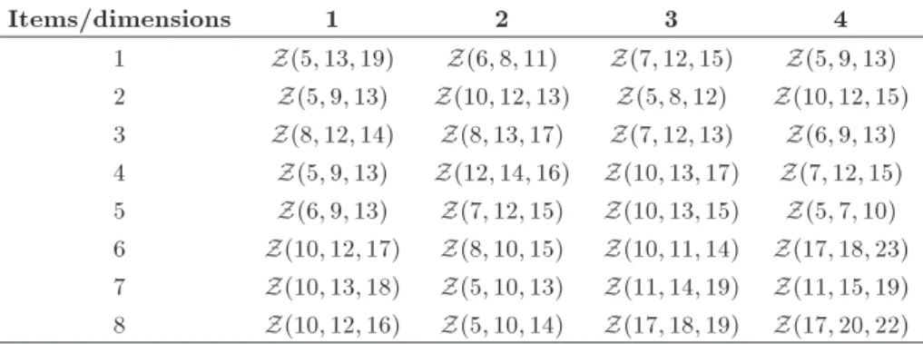
Additionally, all weights, ij, of each item in each
dimension are listed in Table 1. Let items I1, I3, I5,
and I7 be considered for discount with the minimum
weights as 70%, 80%, 85%, and 90% of the total available objects, respectively. So, mathematically, m1 = 0:7, m3 = 0:8, m5 = 0:85, and m7 = 0:9. The
total discount is D = 6. We assume that similar to the item values and knapsack capacities, the discounts are also zigzag uncertain variables, which are listed as
Table 1. The weights ijof each item in each dimension.
Items/dimensions 1 2 3 4
1 Z(5; 13; 19) Z(6; 8; 11) Z(7; 12; 15) Z(5; 9; 13) 2 Z(5; 9; 13) Z(10; 12; 13) Z(5; 8; 12) Z(10; 12; 15) 3 Z(8; 12; 14) Z(8; 13; 17) Z(7; 12; 13) Z(6; 9; 13) 4 Z(5; 9; 13) Z(12; 14; 16) Z(10; 13; 17) Z(7; 12; 15) 5 Z(6; 9; 13) Z(7; 12; 15) Z(10; 13; 15) Z(5; 7; 10) 6 Z(10; 12; 17) Z(8; 10; 15) Z(10; 11; 14) Z(17; 18; 23) 7 Z(10; 13; 18) Z(5; 10; 13) Z(11; 14; 19) Z(11; 15; 19) 8 Z(10; 12; 16) Z(5; 10; 14) Z(17; 18; 19) Z(17; 20; 22)
follows:
1 Z(3; 4; 5); 2 Z(4; 6; 8);
3 Z(5; 6; 7); 4 Z(8; 9; 10);
5 Z(7; 8; 9); 6 Z(5; 6; 7);
7 Z(4; 7; 10); 8 Z(6; 8; 10):
According to Theorem 4, the expected value model for UMKP is equivalent to the following one:
max
8
X
j=1
xj
Z 1
0 1 j ()d;
subject to:
8
X
j=1
xj
Z 1
0 1
ij ()d
Z 1
0 1 i ()d;
for i = 1; 2; 3; 4;
8
X
j=1
yj
Z 1 0 F
1
j ()d D;
xj 2 f0; 1g; yj 2 f0; 1g; for j = 1; 2; ; 8. (7)
Taking by LINGO, we obtain the optimal solution to Model (7) as follows:
(x1; x2; x3; x4; x5; x6; x7; x8)T=(0; 0; 0; 1; 1; 1; 0; 1)T;
i.e. the decision-maker should carry goods 4, 5, 6, and 8 into the bag, and the expected maximum total value of the items that can be carried in the bag is 116.
Assume that the condence levels are = = = 0:9. According to Theorem 5, the chance-constrained programming model for UMKP is equiv-alent to the following one:
max V;
subject to:
8
X
j=1
xjj1(0:1) V;
8
X
j=1
xj ij1(0:9) i1(0:1); for i = 1; 2; 3; 4,
8
X
j=1
yjFj 1(0:1) D;
xj2 f0; 1g; yj2 f0; 1g; for j = 1; 2; ; 8: (8)
Using LINGO software, we obtain the optimal solution to Model (8) as follows:
(x1; x2; x3; x4; x5; x6; x7; x8)T=(0; 0; 0; 1; 1; 1; 0; 1)T;
i.e. the decision-maker should carry goods 4, 5, 6, and 8 into the bag, and the best objective value is 110.4. Since the objective of the chance-constrained programming model is a function of parameter , the sensitivity of the optimal objective can be investigated with respect to dierent parameters. The following predetermined condence levels are selected to test the sensitivity:
= 0:1; 0:2; 0:3; 0:4; 0:5; 0:6; 0:7; 0:8; 0:9; 0:95: The other predetermined condence levels are set as follows:
= = 0:9:
By choosing dierent condence levels, , we obtain Table 2. From Table 2, we nd out that has an eect on the optimal solutions, so that the total weight of the UMKP increases when the condence level decreases, which just coincides with Theorem 6. For understanding this results better, Figure 3 is given.
Table 2. List of -maximum pack when = = 0:9.
1 -maximum pack V 1 -maximum pack V
0.95 0.05 (4, 5, 6, 8) 109 0.5 0.5 (4, 5, 6, 8) 116 0.9 0.1 (4, 5, 6, 8) 110.4 0.4 0.6 (2, 3, 6, 8) 117.2 0.8 0.2 (4, 5, 6, 8) 111.8 0.3 0.7 (2, 3, 6, 8) 118.4 0.7 0.3 (4, 5, 6, 8) 113.2 0.2 0.8 (2, 3, 6, 8) 119.6 0.6 0.4 (4, 5, 6, 8) 114.6 0.1 0.9 (2, 3, 6, 8) 120.8
Figure 3. The sensitivity of the optimal value with dierent of Example 3.
Example 4. To further show the application of the models, more complex experiments have been done. Suppose that there are sixteen items and eight knap-sacks. Let m1= 0:7, m3= 0:8, m5= 0:85, m7 = 0:9,
m9 = 0:9, m11 = 0:95, m13 = 0:8, m15 = 0:9,
and D = 12. In this numerical experiment, all uncertain parameters are assumed to be independent linear uncertain variables. The relevant uncertain parameters are shown in Tables 3-6.
Based on Theorem 4, the expected value model for UMKP is equivalent to the following model:
Table 3. Values, j, of sixteen items.
j j j j j j j j
1 L(32; 36) 5 L(33; 36) 9 L(34; 40) 13 L(35; 41) 2 L(34; 38) 6 L(34; 36) 10 L(37; 42) 14 L(38; 42) 3 L(32; 39) 7 L(32; 37) 11 L(34; 35) 15 L(31; 36) 4 L(36; 39) 8 L(36; 38) 12 L(41; 44) 16 L(42; 46)
Table 4. Capacities iof eight knapsacks.
i 1 2 3 4
i L(42; 102) L(47; 107) L(50; 120) L(70; 120)
i 5 6 7 8
i L(50; 100) L(40; 115) L(40; 100) L(74; 120)
Table 5. Discount coecients jof sixteen items.
j j j j j j j j
1 L(3; 5) 5 L(3; 6) 9 L(5; 10) 13 L(5; 11) 2 L(4; 6) 6 L(3; 6) 10 L(8; 12) 14 L(8; 13) 3 L(2; 7) 7 L(3; 8) 11 L(3; 12) 15 L(3; 15) 4 L(6; 8) 8 L(6; 11) 12 L(4; 15) 16 L(4; 14)
maxX16
j=1
xj
Z 1
0 1 j ()d;
subject to:
16
X
j=1
xj
Z 1
0 1
ij ()d
Z 1
0 1 i ()d;
for i = 1; 2; ; 8;
16
X
j=1
yj
Z 1
0 F 1
j ()d D;
xj 2 f0; 1g; yj 2 f0; 1g; for j = 1; 2; ; 16. (9)
With the help of mathematical software LINGO, we can solve this 0-1 programming problem (9). The result shows that the decision-maker should carry goods 2, 3, 5, 7, 9, 12, 13, and 14 into the bag, and the expected maximum total value of the items that can be carried in the bag is 296.
Assume that the condence levels are = = = 0:9. Based on Theorem 5, the chance-constrained programming model for UMKP is equivalent to the following one:
max V; subject to:
16
X
j=1
xjj1(0:1) V;
16
X
j=1
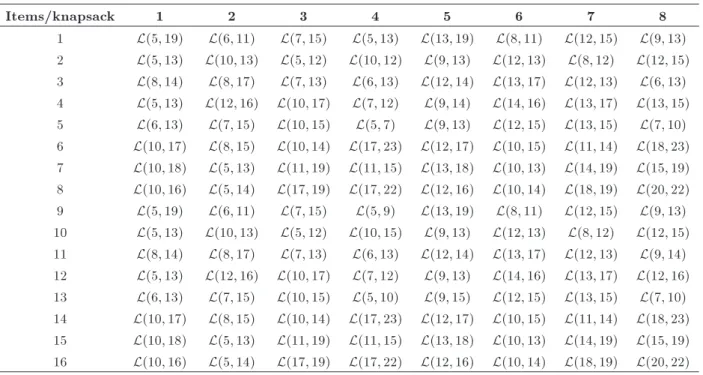
Table 6. Weights, ij, of each item in each knapsack.
Items/knapsack 1 2 3 4 5 6 7 8
1 L(5; 19) L(6; 11) L(7; 15) L(5; 13) L(13; 19) L(8; 11) L(12; 15) L(9; 13) 2 L(5; 13) L(10; 13) L(5; 12) L(10; 12) L(9; 13) L(12; 13) L(8; 12) L(12; 15) 3 L(8; 14) L(8; 17) L(7; 13) L(6; 13) L(12; 14) L(13; 17) L(12; 13) L(6; 13) 4 L(5; 13) L(12; 16) L(10; 17) L(7; 12) L(9; 14) L(14; 16) L(13; 17) L(13; 15) 5 L(6; 13) L(7; 15) L(10; 15) L(5; 7) L(9; 13) L(12; 15) L(13; 15) L(7; 10) 6 L(10; 17) L(8; 15) L(10; 14) L(17; 23) L(12; 17) L(10; 15) L(11; 14) L(18; 23) 7 L(10; 18) L(5; 13) L(11; 19) L(11; 15) L(13; 18) L(10; 13) L(14; 19) L(15; 19) 8 L(10; 16) L(5; 14) L(17; 19) L(17; 22) L(12; 16) L(10; 14) L(18; 19) L(20; 22) 9 L(5; 19) L(6; 11) L(7; 15) L(5; 9) L(13; 19) L(8; 11) L(12; 15) L(9; 13) 10 L(5; 13) L(10; 13) L(5; 12) L(10; 15) L(9; 13) L(12; 13) L(8; 12) L(12; 15) 11 L(8; 14) L(8; 17) L(7; 13) L(6; 13) L(12; 14) L(13; 17) L(12; 13) L(9; 14) 12 L(5; 13) L(12; 16) L(10; 17) L(7; 12) L(9; 13) L(14; 16) L(13; 17) L(12; 16) 13 L(6; 13) L(7; 15) L(10; 15) L(5; 10) L(9; 15) L(12; 15) L(13; 15) L(7; 10) 14 L(10; 17) L(8; 15) L(10; 14) L(17; 23) L(12; 17) L(10; 15) L(11; 14) L(18; 23) 15 L(10; 18) L(5; 13) L(11; 19) L(11; 15) L(13; 18) L(10; 13) L(14; 19) L(15; 19) 16 L(10; 16) L(5; 14) L(17; 19) L(17; 22) L(12; 16) L(10; 14) L(18; 19) L(20; 22)
16
X
j=1
yjFj 1(0:1) D;
xj 2 f0; 1g; yj 2 f0; 1g; for j = 1; 2; ; 16: (10)
By using the mathematical software LINGO, the op-timal solution to Model (10) can be obtained as x1=
x3 = x4 = x7 = x9 = x11 = x13 = x15 = 1, and the
other remaining variables are equal to 0. The optimal value of the objective is equal to 294.6.
If the weights, values, and capacities are general uncertain variables, then it is dicult for us to obtain their uncertainty distributions. Therefore, we can use uncertain statistics [21] to determine the uncertainty distribution. With the help of the designed ques-tionnaire survey, the uncertainty distribution can be determined from the expert's experimental data by using the principle of least squares, the method of moments, the Delphi method, and so on [33].
6. Conclusions and future research
In the real-life industrial engineering applications, we usually encounter the uncertain factors due to lack of observed data about the unknown state of nature. Dierent from previous studies in indeterminacy envi-ronment, this paper mainly investigated multidimen-sional knapsack problem under uncertain environment with discount constraint, where the weights, values, and capacities of each item were depicted as uncertain variables. This work provided signicant contributions to the existing research in the area of uncertain net-work optimization in which the relevant parameters
might be characterized by uncertain variables and have signicant implications in the real-world industrial engineering applications.
The main contributions of this paper include the following three aspects. Firstly, in order to deal with uncertain factors in multidimensional knapsack problem, the uncertainty theory was introduced into the problem under the light of uncertain environment. Secondly, two types of mathematical models for uncer-tain multidimensional knapsack problem were proposed according to two kinds of decision criteria, i.e. the expected value and the critical value criteria. We found out that the maximum value of chance-constrained pro-gramming model was actually decreasing with respect to the predetermined condence level. Thirdly, some numerical examples were given to show the applications of the proposed models. In the numerical examples, we employed two kinds of uncertain variables, i.e. linear uncertain variables and zigzag uncertain variables, to characterize the weights, values, and capacities of the multidimensional knapsack problem. The numerical results illustrated that the proposed models are feasible and ecient for solving the multidimensional knapsack problem with uncertain parameters.
It should be noted that the proposed uncertain programming models in this paper have their unique advantages; that is, they can be easily transformed into their corresponding deterministic equivalent model which can be solved by the classical methods conve-niently. In spite of these advantages, a few issues need to be addressed in the future. For example, we can continue to study the minimum weight dominating set problem and the maximum bi-section problem in
uncertain environment within the axiomatic framework of uncertainty theory. In addition, the current work can be extended to the uncertain random environ-ment [34,35] where uncertainty and randomness coexist in a system. What's more, the situation in which the decision-makers adopt the minimax regret crite-rion [32,36] to make the decisions in the uncertain mul-tidimensional knapsack problem might be considered. While these issues beyond the scope of the present study, we believe they can be potential avenues for future studies.
Acknowledgments
This work was supported by the National Natu-ral Science Foundation of China (No. 71671135), the Natural Science Foundation of Hubei Province (No. 2014CFC1096), the 2014 Key Project of Hubei Provincial Department of Education (No. D20142903), the Projects of the Humanity and Social Science Foundation of Ministry of Education of China (No. 13YJA630065), and the Key Project of Hubei Provin-cial Natural Science Foundation (No. 2015CFA144).
References
1. Rahmani, D., Yousei, A. and Ramezanian, R. \A new
robust fuzzy approach for aggregate production plan-ning", Scientia Iranica, 21(6), pp. 2307-2314 (2014).
2. Tabrizi, B., Tavakkoli-Moghaddam, R. and Ghaderi,
S. \A two-phase method for a multi-skilled project scheduling problem with discounted cash ows", Sci-entia Iranica, 21(3), pp. 1083-1095 (2014).
3. Partovi, F. and Seifbarghy, M. \Service centers
lo-cation problem considering service diversity within queuing framework", Scientia Iranica, 22(3), pp. 1103-1116 (2015).
4. Ramezani, M., Kimiagari, A. and Karimi, B.
\Inter-relating physical and nancial ows in a bi-objective closed-loop supply chain network problem with uncer-tainty", Scientia Iranica, 22(3), pp. 1278-1293 (2015).
5. Freville, A. \The multidimensional 0-1 knapsack
prob-lem: An overview", Eur. J. Oper. Res., 155(1), pp. 1-21 (2004).
6. Henig, M. \Risk criteria in a stochastic knapsack
problem", Oper. Res., 38(5), pp. 820-825 (1990).
7. Kleywegt, A. and Papastavrou, J. \The dynamic and
stochastic knapsack problem", Oper. Res., 46(1), pp. 17-35 (1998).
8. Kosuch, S. \Approximability of the two-stage
stochas-tic knapsack problem with discretely distributed weights", Discret. Appl. Math., 165, pp. 192-204 (2014).
9. Feng, T. and Hartman, J. \The dynamic and stochastic
knapsack problem with homogeneous-sized items and postponement options", Naval Res. Logist., 62(4), pp. 267-292 (2015).
10. Han, J., Lee, K., Lee, C., Choi, K. and Park, S.
\Ro-bust optimization approach for a chance-constrained binary knapsack problem", Math. Program., 157(1), pp. 277-296 (2016).
11. Gibson, M., Ohlmann, J. and Fry, M. \An agent-based
stochastic ruler approach for a stochastic knapsack problem with sequential competition", Comput. Oper. Res., 37(3), pp. 598-609 (2010).
12. Merzifonluoglu, Y., Geunes, J. and Romeijn, H. \The
static stochastic knapsack problem with normally dis-tributed item sizes", Math. Program., 134(2), pp. 459-489 (2012).
13. Okada, S. and Gen, M. \Fuzzy multiple choice
knap-sack problem", Fuzzy Sets Syst., 67(1), pp. 71-80 (1994).
14. Changdar, C., Mahapatra, G. and Pal, R. \An
im-proved genetic algorithm based approach to solve constrained knapsack problem in fuzzy environment", Expert Syst. Appl., 42(4), pp. 2276-2286 (2015).
15. Changdar, C., Mahapatra, G. and Pal, R. \An ant
colony optimization approach for binary knapsack problem under fuzziness", Appl. Math. Comput., 223, pp. 243-253 (2013).
16. Chen, S. \Analysis of maximum total return in the con-tinuous knapsack problem with fuzzy object weights", Appl. Math. Modell., 33(7), pp. 2927-2933 (2009).
17. Baykasoglu, K. and Ozsoydan, F. \An improved rey
algorithm for solving dynamic multidimensional knap-sack problems", Expert Syst. Appl., 41(8), pp. 3712-3725 (2014).
18. Kasperski, A. and Kulej, K. \The 0-1 knapsack
prob-lem with fuzzy data", Fuzzy Optimization Decis. Mak., 6(2), pp. 163-172 (2007).
19. Kahneman, D. and Tversky, A. \Prospect theory: An
analysis of decision under risk", Econometrica, 47(2), pp. 263-292 (1979).
20. Liu, B. \Why is there a need for uncertainty theory", J. Uncertain Syst., 6(1), pp. 3-10 (2012).
21. Liu, B., Uncertainty Theory: A Branch of
Mathemat-ics for Modeling Human Uncertainty, Springer, Verlag, Berlin (2010).
22. Liu, B., Uncertainty Theory, 2nd Edn., Springer,
Verlag, Berlin (2007).
23. Peng, J. and Zhang, B. \Knapsack problem with
uncertain weights and values", http://orsc.edu.cn/ online/120422.pdf (2012).
24. Zhang, B. and Peng, J. \Uncertain programming
model for uncertain optimal assignment problem", Appl. Math. Modell., 37(9), pp. 6458-6468 (2013).
25. Gao, Y. \Shortest path problem with uncertain arc
length", Comput. Math. Appl., 62(6), pp. 2591-2600 (2011).
26. Gao, Y., Yang, L. and Li, S. \Uncertain models
on railway transportation planning problem", Appl. Math. Modell., 40(7-8), pp. 4921-4934 (2016).
27. Liu, Z., Zhao, R., Liu, X. and Chen, L. \Contract de-signing for a supply chain with uncertain information based on condence level", Appl. Soft Comput., 56, pp. 617-631 (2017). DOI: 10.1016/j.asoc.2016.05.054 (2016).
28. Liu, B., Theory and Practice of Uncertain
Program-ming, 2nd Edn., Springer, Verlag, Berlin (2009).
29. Peng, J., Zhang, B. and Li, S. \Towards uncertain
network optimization", J. Uncertainty Anal. Appl., 3(4), pp. 1-19 (2015).
30. Liu, B. \Some research problems in uncertainty
the-ory", J. Uncertain Syst., 3(1), pp. 3-10 (2009).
31. Charnes, A. and Cooper, W. \Chance-constrained
programming", Manage. Sci., 6(1), pp. 73-79 (1959).
32. Kasperski, A. and Zielinski, P. \Minmax regret
ap-proach and optimality evaluation in combinatorial op-timization problems with interval and fuzzy weights", Eur. J. Oper. Res., 200(3), pp. 680-687 (2010).
33. Wang, X., Gao, Z. and Guo, H. \Uncertain hypothesis
testing for two experts' empirical data", Math. Com-put. Model., 55(3-4), pp. 1478-1482 (2012).
34. Liu, Y. \Uncertain random variables: A mixture of
uncertainty and randomness", Soft Comput., 17(4), pp. 625-634 (2013).
35. Liu, Y. \Uncertain random programming with
appli-cations", Fuzzy Optimization Decis. Mak., 12(2), pp. 153-169 (2013).
36. Kasperski, A. and Zielinski, P. \A 2-approximation
algorithm for interval data minmax regret sequencing
problems with the total ow time criterion", Oper. Res. Lett., 36(3), pp. 343-344 (2008).
Biographies
Li Cheng is currently a Master Candidate of College of Mathematics and Physics at Huanggang Normal Uni-versity, Hubei, China. Her research interests focus on uncertainty theory and its application to combinatorial optimization and higher education management. Congjun Rao received his PhD degree in Huazhong University of Sciences and Technology, China. Now, he is an Associate Professor at Huanggang Normal University, Hubei, China. His general research topics of interest include: uncertainty theory, management decision-making, etc. He has published more than 50 papers in various journals, where 22 papers are indexed by SCI and SSCI.
Lin Chen received his MS degree in Applied Math-ematics from Shanghai Normal University in 2015. Now, he is a PhD candidate in the College of Man-agement and Economics, Tianjin University, China. His research interests include uncertain theory and its application to supply chain management and uncertain network optimization. His recent studies have been published in International Journal of Production Re-search, Applied Soft Computing, International Journal of Systems Science, and Journal of Intelligent Manu-facturing, etc.