Sharif University of Technology
Scientia IranicaTransactions B: Mechanical Engineering www.scientiairanica.com
Surface tension simulation of free surface ows using
smoothed particle hydrodynamics
M. Ordoubadi
, M. Yaghoubi and F. Yeganehdoust
School of Mechanical Engineering, Shiraz University, Shiraz, Iran.Received 15 February 2016; received in revised form 29 May 2016; accepted 28 June 2016
KEYWORDS SPH method; Free surface ows; Surface tension; Continuum surface force.
Abstract. SPH method is one of the most used numerical mesh-free methods in CFD simulations which can easily model problems with free surfaces. Considering the importance of surface tension in most engineering applications and the capability of SPH method in simulating free surfaces, a single-phase method for implementing surface tension is introduced in this study. Unlike time-consuming multi-phase simulations, this method does not need to model the second lighter uid, which reduces the CPU-time and memory requirements substantially. Mirror imaginary particles are used near the free surface to obtain surface properties such as surface normal vector and curvature, which are required in surface tension calculation. The advantages of using these imaginary particles are explained qualitatively through the use of some examples of droplet dynamics. This method is applied to several benchmark problems in surface tension simulations, and acceptable results are obtained.
© 2017 Sharif University of Technology. All rights reserved.
1. Introduction
For uid ow simulations, where sharp interfacial cur-vatures are present, surface tension plays an important role in shaping and maintaining the interface between the immiscible phases. Surface tension is the main driving force in the formation of rain droplets, bubbles, guttation, and water beading on the leaves and is of signicance in technological processes such as spray coating, fuel spray, painting, and ink-jet printing.
Generally, one can study interfacial phenomena based on two approaches: macroscopic and microscopic viewpoints. In the former, the analyst is concerned with the macroscopic eects and properties such as uid density, viscosity, and surface tension coecient. In the latter, properties, such as molecular mass and molecular interactions, are the main variables which dene the total surface tension force. The properties
*. Corresponding author.
E-mail address: mnordoubadi@shirazu.ac.ir (M. Ordoubadi)
in both viewpoints are related to each other, but each viewpoint requires dierent numerical procedures. In this study, macroscopic view is of signicance.
Dierent methods have been used to implement surface tension in the grid-based numerical methods. The most utilized method is the Continuum Surface Force (CSF) method proposed by Brackbill et al. [1]. The calculation of surface curvature and normal vectors is required in CSF, which is traditionally accomplished through the use of a color function requiring a second phase near the interface. A macroscopic force is then calculated for the cells near the interface proportional to the surface curvature. The other popular method is the Continuum Surface Stress (CSS) method [2]. The surface force is calculated from a capillary pressure tensor which, in turn, is calculated from the surface normal. There is no need to determine the curvature explicitly in this method, making it less error-prone near sharp and under-resolution corners. CSS method also requires a color function to obtain the surface normal vectors.
Smoothed Particle Hydrodynamics (SPH) is one of the most popular mesh-free methods used excessively in simulating uid ow and computational uid dy-namics. There is no need to track the surface in SPH, making it a desirable scheme in simulating free surface ows [3] in contrast to the grid-based methods which require a multi-phase solution or the use of moving mesh algorithms for modeling such problems. This inherent property of SPH also makes it attractive in simulating interfacial phenomena and surface tension, resulting in dierent implementations of the surface tension eects on SPH. Surface tension is generally applied in two ways in the SPH formulation. The rst method is the use of macroscopic point of view such as CSF [4]. The second method is the use of inter-particle attraction and repulsions and/or van der Waals equation of state [5].
The rst method requires calculation of surface normal vectors and surface curvature explicitly. The surface tension force is obtained from the surface ten-sion coecient and surface curvature in the direction of surface normal. Morris [4] used CSF method in conjunction with SPH for simulating surface tension. He used a color function similar to the one used in grid-based schemes to obtain surface normal and curvatures of interface between phases having low density and viscosity ratios. Hu and Adams [6] extended this two-phase method to simulate surface tension for high density and viscosity ratios. Yeganehdoust et al. [7] enhanced this method to simulate droplet dynamics for high density and viscosity ratios; they also proposed a method to model dierent problems including static and dynamic contact angles.
The second method involves the use of molecular data in simulating surface tension, but that needs to be calibrated for the simulation of real uids. A van der Waals equation of state is used in this method for calculating the pressure eld. A cohesive pressure term is present in this equation of state, which cancels out the inner particles of the uid, but has a net value normal to the interface corresponding to the surface tension eects [8,9]. Tartakovsky and Meakin [10] added an interparticle attractive and repulsive force to this model to make it capable of modeling dierent wetting eects. This method is a suitable choice for modeling surface tension in free surface ows, but it requires cumbersome calibrations for physical properties.
For most practical two-phase applications without shear gas ow, where surface tension is important, the eect of the gas phase is negligible. Hence, the use of a single-phase method is desirable in such cases due to considerable lower memory requirement and CPU time. A multi-phase SPH simulation requires days to run, but a single-phase simulation can give comparable results in hours.
There are very limited free surface applications of the CSF method in SPH formulations compared to the vast multi-phase studies conducted on particle meth-ods. Zhang [11] used geometric interface reconstruction to obtain surface normal and curvatures to calculate surface tension using CSF formulation in single-phase SPH simulations having free surfaces. This method requires complicated programming and diers from the traditional CSF method in a sense that surface properties are not calculated from the derivatives of the color function. Another rather recent study on single-phase simulation of surface tension in particle methods was proposed by Khayyer et al. [12,13] in which they wisely obtained the curvature from direct second-order derivation of color function resulting in a Laplacian formulation with relevant approximation of boundary integrals. Tsuruta et al. [14] proposed the use of MPS and ISPH for free-surface boundary conditions. They implemented projection-based particle methods for moving particle semi-implicit along with the in-compressible SPH methods to handle the free surface. Their new method, called Space Potential Particle (SPP), reproduced physical motions of particles around free surface through a particle-void interaction. In this way, the issue of incomplete compact support is answered. Terissa et al. [15] presented a basic approach for simulating liquid droplet with surface tension in three dimensions using SPH method. They applied the surface tension on the boundary particles of liquid using Free-Surface Detection algorithm in which the particle on the boundary was detected dynamically. They simulated droplet phenomena with the basic method of SPH for uid modeling along with the combination of 3D Free-Surface Detection algorithm with MLS method. Aly et al. [16] simulated surface tension and an eddy viscosity using incompressible smoothed particle hydrodynamics method. In addi-tion, they presented a source term for pressure Poisson equation as a stabilizer for robust simulations in which a smoothed pressure distribution was generated and kept the total volume of uid constant. For decreasing computational costs, surface tension force in the free surface ow was considered without a direct modeling of surrounding air. They simulated the eects of the eddy viscosity with a uid-uid interaction. They concluded that the surface tension model can handle free surface tension problems including high curvatures. In this study, an alternative new single-phase SPH method is proposed to calculate surface tension from CSF formulations suitable for free surface simulations with the use of some imaginary mirror particles near the surface. The use of this kind of imaginary or mirror particles near the interface has been previously used in SPH literature for other applications [17,18], but their eects on simulating surface tension have not been studied. Some 2D benchmark problems
are solved to check the applicability of the developed method, including the oscillation of a square droplet into a circle, head-on and o-center coalescence of two circular droplets, and the impact of a water droplet on a wet bed. The results are compared with analytical as well as VOF results of interFoam solver available in the OpenFOAM program. Good agreement is observed between the results.
2. Governing equations
SPH method is a Lagrangian mesh-free method; hence, the governing equations are all written in the La-grangian frame of reference. Governing equations in this study are the conservation of mass and momentum. Conservation of mass equation is as follows:
D
Dt = r:~V ; (1)
where is the density, and ~V is the velocity vector. The momentum equation in direction for an incom-pressible ow is written in Lagrangian form as follows:
Du
Dt = 1
rp + r
r:~V+1F; (2)
where p is the local static pressure, is the kinematic viscosity, and Fis the summation of all external forces
per unit volume in direction, including gravity and surface tension.
In CSF method, the surface tension force per unit volume is calculated from [1]:
~Fs= (^n + rs) s; (3)
where is the coecient of surface tension, is the surface curvature, ^n is the unit normal vector to the interface, rs is the surface gradient, and s is the
surface Dirac delta function with peak value on the surface. The second term on the right-hand side of Eq. (3) is due to the spatial surface tension variations which give rise to the Marangoni eect. For simulations with constant surface tension values, this term is zero. In multi-phase simulations, each phase is given a color function value c. For example, the gas phase has color function value equal to 1, and the liquid phase has a value equal to 0. Surface normal vector is then obtained from:
~n = rc: (4)
Unit normal vector and surface curvature are also obtained, respectively, as follows:
^n = ~n
j~nj; (5)
= r ^n: (6)
Considering the fact that rc is theoretically zero far from the interface and has a maximum value near this region, surface Dirac delta function can also be obtained from:
s= j~nj: (7)
3. SPH method
The main idea behind SPH mesh-free method is to use integral representation of a function as follows:
f (~x) = Z
f (~x0) (~x ~x0) d~x0; (8)
where is the domain of the integration, and is the Dirac function. Although Eq. (8) holds exactly true, it cannot be used from a computational point of view, because the entire physical domain contributes to the value of any function at any point in the space. In order to compensate for this problem, the Dirac function is approximated by a normalized function, called the kernel function, W (~x ~x0; h), which is a
function of the distance from the point at which the value is to be calculated and smoothing length, h. The smoothing length is related to the distance at which particles aect each other and is held constant in most SPH simulations, usually equal to 1.2 times the initial particle spacing. By approximating the Dirac function by a kernel function, integral representations of a function and its derivative can be shown below [3]:
f (~x) Z
f (~x0) W (~x ~x0; h) d~x0; (9)
r f (~x) Z
f (~x0) rW (~x ~x0; h) dx0: (10)
A kernel function should satisfy some conditions in its support domain h (the support domain of a kernel is the distance in which particles can aect each other) in order for Eqs. (9) and (10) to be as accurate as possible. For example, it should be a normalized, even and decreasing function which should converge to the Dirac function as h ! 0 [19]. For the simulations conducted in this study, Quintic kernel function gave ecient and stable results. This kernel, also called the Wendland function, is shown below [20]:
W (~x ~x0; h)
= (
D(1 + 2q) 1 q24 if 0 q 2
0 else (11)
The physical domain is then discretized by the use of some material points or particles. These particles usually have constant mass and move according to the local ow velocity at each time-step and carry the physical properties of the uid such as density, pressure, temperature, etc. By applying this particle approximation to Eqs. (9) and (10), SPH represen-tation of a function and its derivative is obtained as follows:
f (~xi) = N
X
j=1
mj
j f (~xj) Wij; (12)
r f (~xi) = N
X
j=1
mj
j f (~xj) rWij; (13)
where i is the particle at which the function is being discretized, j corresponds to all the particles in the support domain of i, including particle i itself, mjis the
mass of particle j and Wij = W (~xi ~xj; h). The above
relations are the most straightforward SPH representa-tions of a function and its derivative. Considering the physical aspects of the function being discretized, with some simple algebraic operations, other forms can be obtained by these equations. For example, the pressure gradient in the momentum equation can be discretized in an asymmetric form which ensures conservation of linear momentum as follows:
rp (~xi) = i N
X
j=1
mj pi2 i +
pj
2 j
!
riWij: (14)
The other important term that should be discretized in the momentum equation is the viscous diusion term, which contains the second derivatives of velocity components. The second derivative can be either discretized directly from Eq. (13) which introduces the second derivative of the kernel function or be approximated with the combination of SPH and nite dierence operations [21]. The use of the second derivatives of the kernel function can cause spatial instabilities and reduce the accuracy of the solution, especially for the lower degree kernel functions. Hence, it is a common practice in SPH literature to discretize the second derivatives from the latter method. Viscous diusion term used in this study is the one proposed by Cleary and Monaghan [22] shown below:
r r~V
i= N
X
j=1
mj 8i+ j i+ j
~Vij ~rij
~r 2 ij + 2
! riWij:
(15) With the use of Eqs. (14) and (15), one can easily solve momentum equation considering pressure to be known. Pressure is obtained by two methods in SPH simu-lations for incompressible ows. The rst and more
traditional method is called the Weakly Compressible SPH (WCSPH), which considers the uid to be slightly compressible and assigns to it a weakly compressible equation of state [3,23]. The pressure can then be obtained directly from this equation of state which is a function of density alone. The small compressibility is added to the ow by assigning an articial speed of sound lower than the real value. For most SPH simula-tions, the speed of sound is calibrated to allow around 1% compressibility. In the other method called the Incompressible SPH (ISPH), projection method is used to obtain the pressure Poisson equation. The solution to this equation guarantees the exact incompressibility. ISPH method is proved to be more spatially stable, accurate, and computationally ecient [24-26], while WCSPH is very simple to program and requires no solution to an elliptical partial dierential equation. WCSPH method is used in this study since the lower accuracy of the pressure eld is not of any major consequence for the surface tension simulations conducted.
The weakly compressible equation of state used in this study is the one used by Monaghan [3] as follows:
Pi= B
i 0 1 ; (16)
where B is a constant parameter which decides the maximum density uctuation or compressibility, 0 is
the reference density, and is a constant number equal to 7 in most SPH studies [3,19]. B is obtained from:
B = c200
; (17)
in which c0 is the speed of sound at reference density
and is usually set to 10 times the maximum ow velocity in order to limit the compressibility of the ow to %1. Morris et al. [27] proposed considering the viscous and body forces in conjunction with the above condition for approximating the value of c0. Hence, the
reference speed of sound is:
c2 0= max
V2 ; V L; F L ; (18)
where V is the reference velocity, is the maximum al-lowable compressibility (%1), L is the reference length scale, and F is the acceleration corresponding to the reference body force.
In order to obtain the pressure eld from the equation of state, one should rst calculate the density of each particle. Density can be either calculated directly by discretizing Eq. (1) or by using the SPH representation of density from Eq. (9), which are called the continuity density and summation density methods, respectively [19]. Summation density method conserves
mass exactly, while continuity density method cannot generally conserve mass [23] even though some correc-tions, such as dierent density lters, can be used to circumvent this problem [28-30]. On the other hand, the continuity density method is generally more stable and accurate in problems containing high velocity free surface ows and impact, such as the Dam break problem, due to the underestimation of density at free surfaces in summation density method originated from the truncated support domain of kernel function. Some kernel correction methods are also proposed to tackle this problem [31].
Even though the use of density lter in continuity density method can lower the inaccuracy instances concerning the conservation of mass, more stable re-sults are obtained using the summation density method (especially, in problems with very low velocities and inertial forces); hence, this method is used throughout the present study.
Using summation density method, density of each particle at each time step can be obtained from:
i= N
X
j=1
mjWij: (19)
By applying kernel normalization in order to circum-vent the truncation at free surfaces, density of each particle can be obtained from [31]:
i= N
P
j=1mjWij N
P
j=1
mj
j
Wij
: (20)
To reduce the truncation errors associated with gra-dients of kernel function in the momentum equation, gradient of the kernel function is corrected, which also ensures the conservation of angular momentum. Complete derivation and formulation of this correction is explained in [31].
4. New free surface CSF implementation scheme
In this section, the new method to simulate surface ten-sion in SPH free surface ows is introduced. The goal of this study is to devise and implement a technique to use CSF method in conjunction with SPH scheme without changing much of the conventional CSF formulations. The rst step in achieving the goal is to use an ecient and accurate surface tracking algorithm to nd the particles located at the free surface. The next step is to nd an approach to obtain the surface properties, such as smoothed color function, normal vector, and curvature near the free surface, in the absence of the
second phase. Eventually, the surface tension force can be obtained using Eq. (3). In the following subsections, each of the above steps is explained thoroughly. 4.1. Surface tracking
One of the most important steps in simulating surface tension in free surface ows is to nd all the particles located at the free surface at each time step. That re-quires an explicit interface tracking, unlike multiphase simulations where the interface between the phases is implicitly obtained from the gradient of color function. One of the most straightforward interface tracking methods is to split a circular area around the particle in question into equal sectors. Then, each of these sectors is checked for uid particles. If all sectors have at least one particle inside, then the particle in question is not located on the free surface; otherwise, the particle is marked as one of the free surface particles [11,32]. In this study, area around each particle is divided into 8 sectors, shown schematically in Figure 1.
In most SPH studies, the radius of particle search-ing is equal to the support domain of the kernel, that is, k0 = k [11,32]. This radius gives acceptable results
in simple surface tension simulations, but for impact problems, such as the coalescence of two droplets, where large particle distortion occurs, it was concluded that an increase in this value is required. In the cases investigated in this study, a radius twice the size of kernel support domain (k0 = 2k = 4) gave accurate
results. Henceforth, this method is called the geometric interface tracking in this study.
Even though the above interface tracking algo-rithm is adequately accurate; however, the correspond-ing CPU eort increases exponentially with the number of uid particles, that is, decreasing the eciency of simulation signicantly. In order to decrease the CPU time, this algorithm is combined with another more ecient, but less accurate interface tracking method.
This method is based on the fact that the absolute value of the divergence of position vector of a particle is approximately equal to 2 if the particle is surrounded completely by other particles; this means that it is not on the free surface [24]. One can easily obtain the divergence of position vector from:
(r ~r)i=XN
j=1
mj
j~rij riWij: (21)
Now, if:
jr ~rji "; (22) then particle i is located on free surface, where " is a user-dened number lower than 2. In this study, " is set equal to 1.7, which gives both accurate and e-cient results. This method is called the mathematical interface tracking in the rest of this study.
As explained, the rst interface tracking algo-rithm is accurate but slow; the second method is not as accurate but is relatively more ecient. By combing these two methods, an accurate and ecient interface tracking method is obtained as follows.
First, mathematical interface tracking is per-formed and particles which satisfy Eq. (22) will be marked. Afterwards, geometric interface tracking is performed only on the particles marked in the last step. By doing so, more time-consuming geometric interface tracking is only performed on a small fraction of parti-cles which decreases the total CPU time signicantly.
It is apparent that only particles which can be detected as the interface particles must have satised Eq. (22) in the rst place. It was observed that for some simulations with very large particle distortion, the value of jr ~rj of interface particles can have larger values than pre-specied " value. In such cases, " value should be increased accordingly.
4.2. Smoothed color function
As mentioned in Section 2, for multi-phase simulations, the interface can be tracked via a color function as-signed to each phase. Other properties of the interface, such as surface normal vector and curvature, are then obtained from this color function. It is noted in [4] that smoothing the color function can give more accurate results of the surface normal vector, and hence surface curvature. The smoothing is done using the SPH interpolation of the color function as:
ci= N
X
j=1
mj
j c 0
jWij; (23)
where c0
j is the color function of particle j before any
smoothing (either 0 or 1). In a single-phase simulation, the eect of free surface can be simulated by assigning
Figure 2. Void creation inside the uid in binary coalescence of two droplets.
the color function of the liquid to 1. By doing so, the smoothed color function obtained for the single-phase simulation from Eq. (23) will be identical to a multi-phase simulation if the color function of the gas phase is equal to zero. In other words, support domain truncation in Eq. (23) takes into consideration the existence of an imaginary gas phase, automatically. The use of the above method in smoothing the color function will detect a free surface wherever a num-ber density of particles is low, regardless of the interface tracking algorithm explained in the last subsection. In most impact problems, some voids can appear inside the uid due to the particle distortion, which can induce invalid free surfaces. Unphysical surface tension forces will then appear in these regions and cause the simulation to break-up completely. An example of the aforementioned particle disorder is shown in Figure 2 of the binary coalescence of two droplets. To remedy this problem, integer variable N is introduced for each particle. This variable can be either 0 or 1. At the start of each time-step, this variable is initialized to 0 for all particles. After the completion of interface tracking, all particles are checked to see if they have any free surface particles inside their support domain (with radius of 2h); if a particle has a free surface neighbor, its N value is changed to 1. All the remaining particles with no free surface particles will retain their initial value equal to zero. Now, for all particles, Eq. (23) is modied as follows:
ci=
8 > > > < > > > :
N
P
j=1 mj
jc
0
jWij N = 1
1 else
(24)
4.3. Normal vector
The next step in calculation of surface tension is obtaining normal vectors of each particle. Normal vector is obtained from the gradient of color function,
as shown in Eq. (4). In this study, due to the fact that the color functions of the lighter and denser uids were substituted as explained in Subsection 4.2, the normal vector is obtained as follows:
~n = rc: (25)
The above equation is discretized in the format used by Morris [4] as follows:
~ni= N
X
j=1
mj
j (cj ci)riWij: (26)
The use of the dierence of color functions in the above equation guarantees that the normal vector will be exactly zero in regions far away from the free surface.
For a single-phase simulation with free surface, Eq. (26) can be used for simple surface geometries with no sharp corners and high curvatures. The curvature can then be computed from Eq. (6) with no further modications. But, for most practical problems, large curvatures will appear during the simulation. In these regions, the kernel support domain is highly truncated which will give very small values of the normal vector, which in turn results in small surface tension values. This diculty will be more severe in the calculation of curvature, where two consecutive derivations of color function are required. To solve this problem and increase the accuracy in the calculation of curvature and surface tension, some imaginary particles are assumed near the free surface which will contribute to the calculation of normal vector and curvature of particles near the free surface. The methodology for locating and implementing these imaginary particles is explained next.
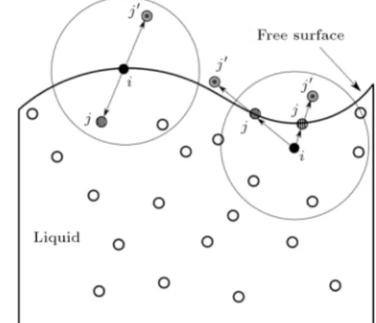
Consider particle i in Eq. (26) with its neighbors presented by j index. Considering if particle i itself is located on the free surface or not, the procedure will be slightly dierent. First, imagine that particle i is located on the free surface. For any particle j in the support domain of i, which is not itself located on the free surface, the position vector between particles i and j is mirrored in the opposite direction. This new vector with its base at i will mark the position of imaginary particle j0. This imaginary particle will
have a contribution in Eq. (26) for particle i, with color function equal to 0, density and mass equal to those of particle i, and riWij0 = riWij. In this
case, imaginary particle j0 is guaranteed to be inside
the support domain of particle i.
Now, consider that particle i is not located on the free surface, but has at least one neighboring particle located on the surface (Ni = 1). For each particle j
located on the free surface inside the support domain of i, vector !ij is again constructed. Now, vectorjj!0 is
constructed equal in magnitude and direction to vector
Figure 3. Treatment of imaginary particles near the free surface.
!ij , so that !
ij0 = !ij +jj!0. Due to the fact that the
length of vector ij!0 is twice the length of!ij , it must
be ascertained that imaginary particle j0 is also inside
the support domain of particle i. If j0 is also inside
the support domain of i, then the contribution of this imaginary particle to Eq. (26) for particle i is applied. It must be noted that in contrary to the previous case, the gradient of kernel function must be evaluated again in this case.
The above procedure for the two dierent scenar-ios is shown schematically in Figure 3.
It must be pointed out that no extra memory is allocated to the imaginary particles; their contributions are immediately applied to the relevant relations when the internal loop calculates the contribution of parti-cle j.
4.4. Surface curvature and surface tension Surface curvature can be obtained from the divergence of unit normal vector discretized in SPH format as follows:
(r ^n)i=
N
X
j=1
mj
j (^nj ^ni) riWij: (27)
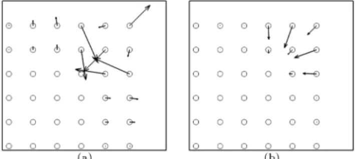
The use of the above relation for all particles without any modication can cause some problems since the unit normal vector is used. The magnitude and direc-tion of normal vector is accurate near the free surface, but has very small values in other regions inside the uid as illustrated in Figure 4(a). The direction of normal vector is not of signicance in these regions where its value is small. The problem arises when the curvature is being calculated, in which the unit normal vector is required and has been normalized by the magnitude of the normal vector. The direction of unit normal vector can be completely erroneous further away from the interface as shown in Figure 4(b). This fact will lower the accuracy in curvature calculation
Figure 4. Normal vectors at the interface of a circular droplet: (a) Normal vectors, (b) unit normal vectors, and (c) ltered unit normal vectors.
of the particles near the interface substantially. To ad-dress this issue, only particles with the accurate normal vectors can be used in the calculation of curvature, and the other particles will be ltered out [4].
To nd particles with reliable normal vectors, integer variable R is dened as follows:
Ri =
8 > < > :
1 j~nij > "0
0 j~nij "0
(28)
in which "0 is equal to 0:01=h. Now, an intermediate
approximation for curvature can be obtained from:
i = (r ^n)i
=
N
X
j=1
min(Ri; Rj)mj
j (^nj ^ni) riWij: (29)
By using the above lter, the kernel support domain of particles will be highly truncated. To circumvent this problem, a kernel gradient correction is applied to Eq. (29) as follows:
i= i=Li; (30)
where:
Li= N
X
j=1
min(Ri; Rj)mj
j Wij: (31)
In the calculation of curvature from Eqs. (29)-(31), the imaginary particles introduced in Section 4.3 are also used to improve the accuracy further. The direction of unit normal vector of the imaginary particles is calculated in the following manner.
If particle i is located on the free surface and have neighbor j not on the surface, an approximate for the unit normal vector of imaginary particle j0 is obtained
from: ^n
j0 = 2^ni ^nj; (32)
and the unit normal vector is:
^nj0 = ^n
j0
j^n
j0j: (33)
Now, consider the case when particle i is not located on the free surface. An approximate unit normal vector for the imaginary particle is:
^n
j0 = 2^nj ^ni; (34)
and the unit normal vector is again obtained from Eq. (33).
After calculation of surface normal vectors and curvature, the acceleration of each particle associated with the surface tension is obtained from:
(~as)i=
i~ni: (35)
4.5. Eects of imaginary particles
As mentioned before, one can simply attempt to model surface tension for free surface ows without the use of introduced mirror particles and just follow the procedure explained in the last subsections. The re-sults obtained might prove accurate enough for simple interfaces, with no sharp corners and sudden changes in the curvature. Nevertheless, for most practical and interesting problems, one is faced with complex geometries. In this part of the study, eects of using imaginary particles are explained and portrayed through some simple visual examples.
First, imagine the interface of a circular droplet. Surface tension must have a maximum value on the surface, should decrease in magnitude by moving away from the free surface, and its direction should be towards the center of the droplet. The surface tension vectors of a section of a circular droplet, with and without the use of imaginary particles, are compared in Figure 5(a) and (b). It should be stated that the magnitudes of these vectors have been rescaled in the two gures. As it is evident from these gures, albeit the direction of the surface tension is acceptable for both cases, the magnitude of the surface tension does not decrease noticeably by moving away from the surface for the simple scheme with no imaginary
Figure 5. Surface tension vectors of a circular droplet: (a) No imaginary particles used, and (b) with imaginary particles.
particles, while this decrease is observable in the presented scheme. The reason is that the particles on the free surface have a smaller number of uid particles in their support domain; hence, the surface tension obtained without the use of any imaginary particles is much smaller.
Next, the surface tension vectors near the sharp corner of a square droplet are inspected for the two methods. Near a sharp corner, surface tension should have the highest value at the tip of the corner and should be smaller further away. The direction of these vectors should be inwards for a convex interface. The surface tension vectors obtained from the simple simulation and the introduced scheme are compared in Figure 6.
It is observed that the magnitude and direction of surface tension vectors are completely erroneous near such a sharp corner if no imaginary particle is used. The direction and magnitude of the vectors for the current scheme is acceptable even though the maximum tension does not occur at the corner. This is due to the fact that the particle exactly located on the corner has a smaller number of imaginary particles associated with it due to its smaller number of uid neighbors.
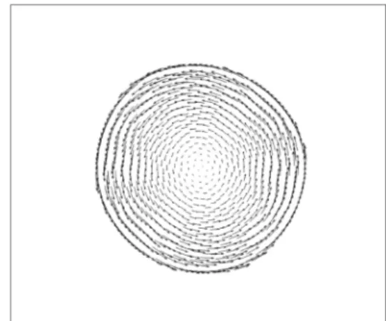
Furthermore, to quantitatively compare the use of the imaginary particles, the curvature values of particles immediately located on a free surface of a circular droplet with respect to horizontal coordinate are calculated and illustrated in Figure 7. Because the
Figure 6. Surface tension vectors near the corner of a square droplet: (a) No imaginary particles used, and (b) with imaginary particles.
Figure 7. The comparison of curvature values on the droplet surface.
circular shape was obtained from the nal deformation of a square droplet, some small disturbances are visible for the particles initially located at the sharp corners. The improvement in curvature calculation with the use of mirror particles is quite considerable, as illustrated in this gure.
5. Results and discussion
In this section, transient computations of some 2D surface tension benchmarks are presented to further evaluate the eectiveness and practicality of the pro-posed single-phase scheme. The rst problem is the transformation and evolution of an initially square-shaped droplet into a circle. The steady-state pressures of the drops are compared with the exact solution, while the transient shape of the droplet is compared with the multi-phase VOF results of OpenFOAM 3.2, available for free in the public domain. Next, results for the head-on and o-center coalescence of two circular droplets are presented, and transient data are compared to the results obtained from VOF simulation. For all the multi-phase simulations, the gas phase is considered to be air.
5.1. The square droplet
One of the most elementary and common benchmarks in the numerical simulation of surface tension is the transformation of a square-shaped droplet into a cir-cular one. In most of the studies in the literature, the physical properties associated with this problem are non-dimensionalized into two numbers: the Weber and Reynolds numbers. A characteristic velocity is needed in the calculation of both of these dimensionless numbers, which is not well-dened in the problem at hand. In order to generalize the simulation and omit any uncertainties, the Ohnesorge number is used for this problem. The problem is solved for three Oh numbers of 0.1, 0.2, and 0.5 for two particle spacings of 2:5e 4m (1640 particles) and 5:0e 4m (441 particles).
The Ohnesorge number, Oh, is a dimensionless number equal to:
Oh = p
We Re =
p
0L0; (36)
where L0 is the characteristic length, Re =0UL 0, and
We = 0U2L0
; U is the characteristic velocity. It is
apparent that in the Ohnesorge number, the unknown characteristic velocity is omitted.
The initial problem setup is shown schematically in Figure 8, and the relevant physical properties and dimensions for the three aforementioned Oh numbers are presented in Table 1. In the fth column of this table, r is the approximated radius of the nal circular droplet which is obtained by assuming that the total
Table 1. Physical properties and dimensions for the square droplet problem. Ohnesorge number 0 (kg/m3) (m2/s) L
0 (m) r = L0=p (m) (N/m)
0.1 1000 1:0e 4 0.01 0.00564 0.1
0.2 1000 1:0e 4 0.01 0.00564 0.025
0.5 1000 1:0e 4 0.01 0.00564 0.004
Figure 8. Initial setup for the square droplet problem.
volume of the droplet will be constant throughout the solution. The external solid wall boundary is simulated in the VOF solution with LB= 10L0.
The steady-state pressure of the nal circular droplets is presented and compared with the pressure obtained from Laplace equation (p = =r) in Table 2. It is observed that the accuracy of the nal central pres-sures is acceptable. To ensure that the time-dependent evolution of the droplet is also correct, the oscillations of the droplet at some time intervals are compared to the results of the VOF simulation conducted via the interFoam solver in the OpenFoam package. The general shape of the droplet in the Ohnesorge number of 0.1 is compared to the volume fraction contours of the VOF simulation in Figure 9. Considerable similarity is observed between these methods at all the instances displayed.
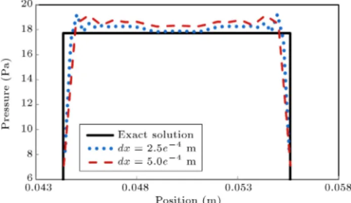
The steady-state pressure proles on the horizon-tal centerline of the droplet with the Ohnesorge number equal to 0.1 are shown in Figure 10. The small pressure uctuations near the free surface are due to the use of summation density method in calculation of the density
Table 2. Steady-state pressure at the center of the nal droplet.
Oh Pexact
(Pa)
Psimulation (Pa)
dx0 = 5:0e 4 m dx0 = 2:5e 4 m
0.1 17.72 18.35 17.83
0.2 4.43 4.57 4.53
0.5 0.71 0.72 0.73
Figure 9. Evolution of a square droplet into a circle for Oh = 0.1. Left: current study, right: VOF simulation.
Figure 10. Final centerline pressure of the droplet for Oh = 0.1.
eld. Although corrected Eq. (20) is used, the support domain truncation still causes such small discrepancies near the surface. The transient oscillations of the average pressure of particles for the Ohnesorge numbers of 0.1, 0.2, and 0.5 are also shown in Figure 11.
It is apparent from Figure 11 that the vibrations of droplets with Oh numbers of 0.1 and 0.2 are under-damped. When Oh is increased to 0.5 though, the vibrations show over-damped characteristics.
The slight oset present between the two spatial resolutions for all Ohnesorge numbers is due to the fact that a larger fraction of particles is located on the free surface in the cases with higher particle spacings. By inspecting Figure 11(a), one can note some small
uc-tuations after t = 0:20 sec for the ne resolution. These unphysical uctuations are due to the parasitic currents which appear in both CSF and CSS methods due to the imbalances induced in the momentum equations [1,2]. Harvie et al. [33] obtained some correlations to predict the maximum value of these currents for volume of uid
Figure 11. Transient average pressure of an initially square shaped droplet for various Ohsenorge numbers.
simulations. Their correlations can well be extended to other methods if expressed qualitatively. They approximated the magnitude of parasitic currents from the balances between inertia, advection and viscous terms with the surface tension. It is shown that the maximum value of these currents is related to:
Parasitic currents /
Surface tension eects Viscous eects
;
Surface tension eects Inertia eects
;
Surface tension eects Advection eects
:
Hence, by decreasing the Ohnesorge number, the eects of these currents increase. Also, it is apparent from the above relation that by approaching the steady-state stationary condition, these currents will prevail. It is also shown in the relations given in the above study [33] that by increasing the spatial resolution, the eects of parasitic currents increase.
According to the above observations, a CSF method (regardless of the numerical implementation method) is error-prone in low velocity simulations of uids with very small Ohnesorge numbers. Also, it is not recommended to increase the spatial resolutions higher than a problem-dependent value.
5.2. Binary head-on collision and coalescence of two circular droplets
Another problem in surface tension studies is the head-on coalescence of two circular droplets at zero gravity conditions. This specic problem diers from the previous case due to the fact that at some time during the simulation, negative curvatures will occur at the bridge formed between the two droplets, as illustrated in Figure 12. At these regions, the surface tension will be directed outwards. A reliable surface tension scheme
Figure 12. Negative curvature at the liquid bridge in binary coalescence of two droplets.
Figure 13. Initial set-up of head-on coalescence problem.
should be able to capture these spatial variations in curvature on the free surface.
In this study, the head-on coalescence of two circular droplets, each with radius of 0.0056 m and 0.0046 m apart, is simulated. Density, kinematic viscosity, and surface tension coecient of the droplets are 1000 kg/m3, 0.0001 m2/s, and 0.025 N/m,
respec-tively. The circular droplets are created from a square droplet of length 0.01 m which is considered to be the characteristic length of this problem. The two droplets approach each other with relative velocity of 0.04 m/s, corresponding to the Reynolds and Weber numbers of 4.0 and 0.64, respectively. The initial distances and velocities are shown schematically in Figure 13.
The coalescence of these two droplets is compared to the multi-phase results of OpenFOAM over some time intervals in Figure 14. Excellent agreement is ob-served between the two methods at all of the presented time snapshots. After the initial impact of the droplets, a narrow liquid bridge is formed between them which has larger local pressure. This pressure gradient causes the bridge to spread in vertical directions creating an elliptical shape. The surface tension will overcome the inertia forces at some point and prevent the droplet from further expansion and will make it contract. The center pressure will increase and the drop will start
Figure 14. Head-on coalescence of two circular droplets. Left: current study, right: VOF simulation.
Figure 15. Horizontal and vertical spans of the head-on coalescence.
to expand horizontally, and the cycle repeats itself in vertical and horizontal directions. After each cycle, the maximum elongation in each direction decreases until a circular droplet is formed. The transient horizontal and vertical dierences between minimum and maximum limits of the droplets (Delta X and Delta Z) are shown in Figure 15. The decay in amplitudes of the vibrations stated above is apparent from this gure. The nal stable droplet is formed slightly earlier by the VOF method due to the viscous loss associated with the gas phase. It is also observed in the VOF results that some air is trapped between the two droplets after the impact. Of course, this air entrapment phenomenon cannot be modeled in the proposed single-phase simulation.
The simulation of this problem using the proposed scheme shows the reliability and practicality of the method in surface tension simulations where sharp and negative curvatures appear. Still, it should be mentioned that by increasing the spatial resolution beyond a certain value, the parasitic currents will make the coalescence of droplets asymmetrical and unstable. The fact that there is no gaseous phase to dampen these currents makes this instability more signicant compared to other multiphase simulations.
5.3. O-center coalescence of two circular droplets
The last problem is the o-center collision and co-alescence of two circular droplets, each with radius of 0.0056 m. The center-to-center vertical distance of the two droplets is equal to 0.0056 m, and they are approaching each other with a relative horizontal velocity of 0.04 m/s. The schematic of this problem is shown in Figure 16. The physical properties are similar to the last problem; hence, the corresponding Reynolds and Weber numbers are also 4.0 and 0.64, respectively. The coalescence process is compared with the results of VOF simulation in Figure 17. Good
Figure 16. Schematic of the o-center coalescence of two circular droplets.
Figure 17. O-center coalescence of two circular droplets. Left: current study, right: VOF.
agreement is visible between the two methods, albeit some distortions are visible on the free surface of the SPH results.
Due to the presence of initial angular momentum in the system, the droplets will begin to rotate around the center of mass of the system. This rotation is illustrated via the velocity vectors at t = 1:00 sec in Figure 18. When the droplet is surrounded by air, such as the VOF simulation, this rotation will eventually decay until the nal droplet reaches stationary condi-tion. In the present single-phase simulation though, this rotation will continue with no resistance. Hence, we can calculate the angular velocity of the system from the conservation of angular momentum:
2 (dVdroplets
oCenter=2) Id= ! Itotal; (37)
where Vdroplets is the horizontal magnitude of the
velocity of each droplet, doCenteris the center-to-center
vertical distance of the two droplets, Id is the moment
of inertia of each circular droplet before impact, Itotalis
the moment of inertia of the nal circular droplet, and ! is its angular velocity. The angular velocity of the
Figure 18. Velocity vectors for the o-center coalescence showing the rotation of the nal droplet at t = 1:00 sec.
nal droplet calculated from Eq. (37) is 3.58 rad/sec, while this value is obtained to be 3.26 rad/sec from the current simulation at t = 1:00 sec. Aside from the apparent numerical errors, this small deviation is due to the fact that CSF method does not conserve linear and angular momenta exactly [2,4].
Like the previous problem, in the VOF results, some air is again entrapped between the droplets, but, unlike the last case, this entrapped air will be eventually gathered at the center of the droplet in a small circular region due to the rotation of the nal droplet. Of course, this entrapment does not happen in our free surface simulation.
5.4. Drop impact on a water bed
So far, all the problems, which have been simulated, contained droplets with high viscosities that prevent the occurrence of some phenomena such as splashing and spray formation. In order to briey illustrate the capability of the proposed surface tension method in low viscosity conditions, the impact of a water droplet on a water surface is also simulated and compared with the studies of Leng [34] and Khayyer et al. [12]. The Laplacian-based surface tension modelling of Khayyer et al. has been explained with more details in [13]. In this case, a water droplet of diameter 2.33 mm collides with the water surface at the velocity of 3.65 m/s resulting in We = 395 and Fr = 639. The droplet breaks up into smaller droplets and splashes o the surface. Two instantaneous snapshots are displayed in Figure 19. Great agreement is observed and the splashing and breaking up of the droplet are also visible. As it can be seen in the second snapshot, some particles will get separated from the rest of the water. This will induce some articial and large surface tensions for these singular particles. In order to stabilize the method in such situations, when a particle does not have enough uid particles in its support domain, surface tension is not computed and is equated to zero.
Figure 19. Droplet splashing over a water bed: (a) Current study, (b) Leng [34], and (c) Khayyer et al. [12].
6. Conclusions
In this study, a single-phase implementation of CSF method in simulating surface tension eects for free surfaces in SPH method is proposed. Unlike the other multi-phase studies where the whole physical domain should be discretized by both liquid and gas particles, in this study, only the liquid domain is needed to be discretized, lowering the memory requirements and CPU time signicantly. Naturally, if the problem at hand is to analyze phenomena, such as shear eects of the gas phase or air entrapment, a multi-phase simulation is required and this study cannot address these issues.
After an accurate and ecient surface tracking, imaginary mirror particles are placed adjacent to the surface. The mirror particles are used in the calculation of surface properties such as surface normal vector and curvature. The impact of using these particles is illustrated through some simple examples, and it is shown that their use has signicant eect on the surface tension, especially near the sharp corners with high curvature. These particles do not require any extra memory requirement and only their contribution is considered.
The proposed scheme is applied to some simple 2D surface tension examples such as the oscillation of a square shaped droplet and binary coalescence of two droplets. The results of the current study show good agreement with exact data as well as results obtained from VOF simulation. It is also observed that by increasing spatial resolution at lower Ohne-sorge numbers, parasitic currents can appear in the simulation. The conservation of angular momentum is also studied via the simulation of o-center coalescence of two droplets. It is conrmed that CSF method cannot conserve momentum exactly. In simulations where conservation of linear and angular momenta is imperative, the use of CSS method is recommended, in which the implementation of the introduced imaginary particles is also straightforward.
Acknowledgments
The authors appreciate support from Iran's National Elite Foundation.
References
1. Brackbill, J.U., Kothe, D.B. and Zemach, C. \A continuum method for modeling surface tension", J. Comput. Phys., 100(2), pp. 335-354 (1992).
2. Lafaurie, B., Nardone, C., Scardovelli, R., Zaleski, S. and Zanetti, G. \Modelling merging and fragmentation in multiphase ows with SURFER", J. Comput. Phys., 113(1), pp. 134-147 (1994).
3. Monaghan, J.J. \Simulating free surface ows with SPH", J. Comput. Phys., 110, pp. 399-406 (1994). 4. Morris, J.P. \Simulating surface tension with
smoothed particle hydrodynamics", Int. J. Numer. Methods Fluids, 33(3), pp. 333-353 (2000).
5. Melean, Y. and Sigalotti, L.D.G. \Coalescence of colliding van der Waals liquid drops", Int. J. Heat Mass Transfer, 48(19-20), pp. 4041-4061 (2005). 6. Hu, X.Y. and Adams, N.A. \A multi-phase SPH
method for macroscopic and mesoscopic ows", J. Comput. Phys., 213(2), pp. 844-861 (2006).
7. Yeganehdoust, F., Yaghoubi, M., Emdad, H. and Ordoubadi, M. \Numerical study of multiphase droplet dynamics and contact angles by smoothed particle hydrodynamics", Appl. Math. Modell., 40(19), pp. 8493-8512 (2016).
8. Nugent, S. and Posch, H.A. \Liquid drops and surface tension with smoothed particle applied mechanics", Phys. Rev. E, 62(4), pp. 4968-4975 (2000).
9. Melean, Y., Sigalotti, L.D.G. and Hasmy, A. \On the SPH tensile instability in forming viscous liquid drops", Comput. Phys. Commun., 157(3), pp. 191-200 (2004).
10. Tartakovsky, A. and Meakin, P. \Modeling of surface tension and contact angles with smoothed particle hy-drodynamics", Phys. Rev. E, 72(2), p. 026301 (2005). 11. Zhang, M. \Simulation of surface tension in 2D and 3D with smoothed particle hydrodynamics method", Journal of Computational Physics, 229(19), pp. 7238-7259 (2010).
12. Khayyer, A., Gotoh, H. and Tsuruta, N. \A novel Laplacian-based surface tension model for particle methods", In 9th SPHERIC International Workshop, Paris (2014).
13. Gotoh, H. and Khayyer, A. \Current achievements and future perspectives for projection-based particle methods with applications in ocean engineering", J. Ocean Eng. Mar. Energy, pp. 1-28 (2016).
14. Tsuruta, N., Khayyer, A. and Gotoh, H. \Space po-tential particles to enhance the stability of projection-based particle methods", Int. J. Comput. Fluid Dyn., 29(1), pp. 100-119 (2015).
15. Terissa, H., Barecasco, A. and Naa, C.F. \Three-dimensional smoothed particle hydrodynamics simu-lation for liquid droplet with surface tension", arXiv Preprint arXiv: 1309.3868, pp. (2013).
16. Aly, A.M., Asai, M. and Sonda, Y. \Modelling of surface tension force for free surface ows in ISPH method", Int. J. Numer. Methods Heat Fluid Flow, 23(3), pp. 479-498 (2013).
17. Schechter, H. and Bridson, R. \Ghost SPH for animat-ing water", ACM Trans. Graphics, 31(4), p. 61 (2012). 18. Jilani, A.N. and Hashemi, S.U. \Numerical investiga-tions on bed load sediment transportation using SPH method", Scientia Iranica, 20(2), pp. 294-299 (2013). 19. Liu, G.R. and Liu, M.B., Smoothed Particle Hydrody-namics: A Meshfree Particle Method, World Scientic (2003).
20. Wendland, H. \Piecewise polynomial, positive denite and compactly supported radial functions of mini-mal degree", Adv. Comput. Math., 4(1), pp. 389-396 (1995).
21. Cummins, S.J. and Rudman, M. \An SPH projection method", J. Comput. Phys., 152, pp. 584-607 (1999). 22. Cleary, P.W. and Monaghan, J.J. \Conduction mod-elling using smoothed particle hydrodynamics", J. Comput. Phys., 148, pp. 227-264 (1999).
23. Monaghan, J.J. \Smoothed particle hydrodynamics", Annu. Rev. Astron. Astrophys., 30, pp. 543-574 (1992). 24. Lee, E.-S., Moulinec, C., Xu, R., Violeau, D., Lau-rence, D. and Stansby, P. \Comparisons of weakly compressible and truly incompressible algorithms for the SPH mesh free particle method", J. Comput. Phys., 227, pp. 8417-8436 (2008).
25. Farhadi, A., Emdad, H., Goshtasebi Rad, E. and Ordoubadi, M. \Modied variable mass incompressible SPH method for simulating internal uid ows", J. Braz. Soc. Mech. Sci. Eng., pp. 1-19 (2015).
26. Ordoubadi, M., Farhadi, A., Yeganehdoust, F., Em-dad, H., Yaghoubi, M. and Goshtasebi Rad, E. \Eu-lerian ISPH method for simulating internal ows", J. Appl. Fluid Mech., 9(3), pp. 1477-1490 (2016). 27. Morris, J.P., Fox, P.J. and Zhu, Y. \Modeling low
Reynolds number incompressible ows using SPH", J. Comput. Phys., 136, pp. 214-226 (1997).
28. Dilts, G.A. \Moving-least-squares-particle hydro-dynamics-I. Consistency and stability", Int. J. Numer. Methods Eng., 44(8), pp. 1115-1155 (1999).
29. Colagrossi, A. and Landrini, M. \Numerical simulation of interfacial ows by smoothed particle hydrodynam-ics", J. Comput. Phys., 191(2), pp. 448-475 (2003).
30. Panizzo, A. and Dalrymple, R. \SPH modelling of underwater landslide generated waves", In Coastal En-gineering Conference, World Scientic, p. 1147 (2004). 31. Bonet, J. and Lok, T.-S. \Variational and momentum preservation aspects of smooth particle hydrodynamic formulations", Comput. Methods Appl. Mech. Eng., 180(1), pp. 97-115 (1999).
32. Dilts, G.A. \Moving least-squares particle hydrody-namics II: Conservation and boundaries", Int. J. Nu-mer. Methods Eng., 48(10), pp. 1503-1524 (2000). 33. Harvie, D.J., Davidson, M. and Rudman, M. \An
analysis of parasitic current generation in volume of uid simulations", Appl. Math. Modell., 30(10), pp. 1056-1066 (2006).
34. Leng, L.J. \Splash formation by spherical drops", J. Fluid Mech., 427, pp. 73-105 (2001).
Biographies
Mani Ordoubadi holds a Master's degree in Me-chanical Engineering, Energy Conversion, from Shiraz University His main research expertise is in computa-tional uid dynamics with focus on multi-phase ows, free surface ows, and surface tension and interfacial phenomena. His numerical experience includes both grid-based and mesh-free methods.
Mahmood Yaghoubi is a Professor of Mechanical Engineering at Shiraz University. He is a fellow member of Academy of Science of Islamic Republic of Iran. His main research interests are convection heat and mass transfer, computational and experimental uid dynamics, phase-change phenomena, solar energy, and engineering education.
Firoozeh Yeganehdoust graduated from School of Mechanical Engineering at Shiraz University, Iran in 2014. Her main areas of research interests include multi-phase ow and surface eects, computational uid dynamics, heat transfer, and applied mathe-matics. Her Master thesis was mainly focused on the investigation of numerical analysis of water drops motion over an inclined surface by SPH method.


![Figure 19. Droplet splashing over a water bed: (a) Current study, (b) Leng [34], and (c) Khayyer et al](https://thumb-us.123doks.com/thumbv2/123dok_us/8377324.2225283/14.892.66.416.148.276/figure-droplet-splashing-water-current-study-leng-khayyer.webp)
