Curves and Surfaces in Geometric Modeling: Theory & Algorithms - Free Computer, Programming, Mathematics, Technical Books, Lecture Notes and Tutorials

(1)

(2)

(3)

Curves and Surfaces

In Geometric Modeling:

Theory And Algorithms

Jean Gallier

Department of Computer and Information Science

University of Pennsylvania

Philadelphia, PA 19104, USA

e-mail:

[email protected]

c

Jean Gallier

Please, do not

reproduce

without permission

of the author

(4)

(5)

iii

To my new daughter Mia, my wife Anne,

(6)

(7)

Preface

This book is primarily an introduction to geometric concepts and tools needed for solving problems of a geometric nature with a computer. Our main goal is to provide an introduc-tion to the mathematical concepts needed in tackling problems arising notably in computer graphics, geometric modeling, computer vision, and motion planning, just to mention some key areas. Many problems in the above areas require some geometric knowledge, but in our opinion, books dealing with the relevant geometric material are either too theoretical, or else rather specialized and application-oriented. This book is an attempt to fill this gap. We present a coherent view of geometric methods applicable to many engineering problems at a level that can be understood by a senior undergraduate with a good math background. Thus, this book should be of interest to a wide audience including computer scientists (both students and professionals), mathematicians, and engineers interested in geometric methods (for example, mechanical engineers). In particular, we provide an introduction to affine ge-ometry. This material provides the foundations for the algorithmic treatment of polynomial curves and surfaces, which is a main theme of this book. We present some of the main tools used in computer aided geometric design (CAGD), but our goal is not to write another text on CAGD. In brief, we are writing about

Geometric Modeling Methods in Engineering

We refrained from using the expression “computational geometry” because it has a well established meaning which does not correspond to what we have in mind. Although we will touch some of the topics covered in computational geometry (for example, triangulations), we are more interested in dealing with curves and surfaces from an algorithmic point of view. In this respect, we are flirting with the intuitionist’s ideal of doing mathematics from a “constructive” point of view. Such a point of view is of course very relevant to computer science.

This book consists of four parts.

• Part I provides an introduction to affine geometry. This ensures that readers are on firm grounds to proceed with the rest of the book, in particular the study of curves and surfaces. This is also useful to establish the notation and terminology. Readers

(12)

proficient in geometry may omit this section, or use it by need. On the other hand, readers totally unfamiliar with this material will probably have a hard time with the rest of the book. These readers are advised do some extra reading in order to assimilate some basic knowledge of geometry. For example, we highly recommend Berger [5, 6], Pedoe [59], Samuel [69], Hilbert and Cohn-Vossen [42], do Carmo [26], Berger and Gostiaux [7], Boehm and Prautzsch [11], and Tisseron [83].

• Part II deals with an algorithmic treatment of polynomial curves (B´ezier curves) and spline curves.

• Part III deals with an algorithmic treatment of polynomial surfaces (B´ezier rectangular or triangular surfaces), and spline surfaces. We also include a section on subdivision surfaces, an exciting and active area of research in geometric modeling and animation, as attested by several papers in SIGGRAPH’98, especially the paper by DeRose et al [24] on the animated character Geri, from the short movie Geri’s game.

• Part IV consists of appendices consisting of basics of linear algebra, certain technical proofs that were omitted earlier, complements of affine geometry, analysis, and dif-ferential calculus. This part has been included to make the material of parts I–III self-contained. Our advice is to use itby need!

Our goal is not to write a text on the many specialized and practical CAGD methods. Our main goal is to provide an introduction to the concepts needed in tackling problems arising in computer graphics, geometric modeling, computer vision, and motion planning, just to mention some key areas. As it turns out, one of the most spectacular application of these concepts is the treatment of curves and surfaces in terms of control points, a tool extensively used in CAGD. This is why many pages are devoted to an algorithmic treatment of curves and surfaces. However, we only provide a cursory coverage of CAGD methods. Luckily, there are excellent texts on CAGD, including Bartels, Beatty, and Barsky [4], Farin [32, 31], Fiorot and Jeannin [35, 36], Riesler [68], Hoschek and Lasser [45], and Piegl and Tiller [62]. Similarly, although we cover affine geometry in some detail, we are far from giving a comprehensive treatments of these topics. For such a treatment, we highly recommend Berger [5, 6], Pedoe [59], Tisseron [83], Samuel [69], Dieudonn´e [25], Sidler [76], and Veblen and Young [85, 86], a great classic. Several sections of this book are inspired by the treatment in one of several of the above texts, and we are happy to thank the authors for providing such inspiration.

(13)

CONTENTS 3 in our use of multilinear tools. As the reader will discover, much of the algorithmic theory of polynomial curves and surfaces is captured by the three words:

Polarize, homogenize, tensorize!

We will be dealing primarily with the following kinds of problems:

• Approximating a shape (curve or surface).

We will see how this can be done using polynomial curves or surfaces (also called B´ezier curves or surfaces), spline curves or surfaces.

• Interpolating a set of points, by a curve or a surface.

Again, we will see how this can be done using spline curves or spline surfaces.

• Drawing a curve or a surface.

The tools and techniques developed for solving the approximation problem will be very useful for solving the other two problems.

The material presented in this book is related to the classical differential geometry of curves and surfaces, and to numerical methods in matrix analysis. In fact, it is often pos-sible to reduce problems involving certain splines to solving systems of linear equations. Thus, it is very helpful to be aware of efficient methods for numerical matrix analysis. For further information on these topics, readers are referred to the excellent texts by Gray [39], Strang [81], and Ciarlet [19]. Strang’s beautiful book on applied mathematics is also highly recommended as a general reference [80]. There are other interesting applications of geom-etry to computer vision, computer graphics, and solid modeling. Some great references are Koenderink [46] and Faugeras [33] for computer vision, Hoffman [43] for solid modeling, and Metaxas [53] for physics-based deformable models.

Novelties

As far as we know, there is no fully developed modern exposition integrating the basic concepts of affine geometry as well as a presentation of curves and surfaces from the algo-rithmic point of view in terms of control points (in the polynomial case). There is also no reasonably thorough textbook presentation of the main surface subdivision schemes (Doo-Sabin, Catmull-Clark, Loop), and a technical discussion of convergence and smoothness.

New Treatment, New Results

(14)

We give an in-depth presentation of polynomial curves and surfaces from an algorith-mic point of view. The approach (sometimes called blossoming) consists in multilinearizing everything in sight (getting polar forms), which leads very naturally to a presentation of polynomial curves and surfaces in terms of control points (B´ezier curves and surfaces). We present many algorithms for subdividing and drawing curves and surfaces, all implemented in Mathematica. A clean and elegant presentation of control points is obtained by using a construction for embedding an affine space into a vector space (the so-called “hat con-struction”, originating in Berger [5]). We even include an optional chapter (chapter 11) covering tensors and symmetric tensors to provide an in-depth understanding of the foun-dations of blossoming and a more conceptual view of the computational material on curves and surfaces. The continuity conditions for spline curves and spline surfaces are expressed in terms of polar forms, which yields both geometric and computational insights into the subtle interaction of knots and de Boor control points.

Subdivision surfaces are the topic of Chapter 9 (section 9.4). Subdivision surfaces form an active and promising area of research. They provide an attractive alternative to spline surfaces in modeling applications where the topology of surfaces is rather complex, and where the initial control polyhedron consists of various kinds of faces, not just triangles or rectangles. As far as we know, this is the first textbook presentation of three popular methods due to Doo and Sabin [27, 29, 28], Catmull and Clark [17], and Charles Loop [50]. We discuss Loop’s convergence proof in some detail, and for this, we give a crash course on discrete Fourier transforms and (circular) discrete convolutions. A glimpse at subdivision surfaces is given in a new Section added to Farin’s Fourth edition [32]. Subdivision surfaces are also briefly covered in Stollnitz, DeRose, and Salesin [79], but in the context of wavelets and multiresolution representation.

A a general rule, we try to be rigorous, but we always keep the algorithmic nature of the mathematical objects under consideration in the forefront.

Many problems and programming projects are proposed (over 200). Some are routine, some are (very) difficult.

Many algorithms and their implementation

Although one of our main concerns is to be mathematically rigorous, which implies that we give precise definitions and prove almost all of the results in this book, we are primarily interested in the repesentation and the implementation of concepts and tools used to solve geometric problems. Thus, we devote a great deal of efforts to the development and implemention of algorithms to manipulate curves, surfaces, triangulations, etc. As a matter of fact, we provide Mathematica code for most of the geometric algorithms presented in this book. These algorithms were used to prepare most of the illustrations of this book. We also urge the reader to write his own algorithms, and we propose many challenging programming projects.

(15)

CONTENTS 5 Not only do we present standard material (although sometimes from a fresh point of view), but whenever possible, we state some open problems, thus taking the reader to the cutting edge of the field. For example, we describe very clearly the problem of finding an efficient way to compute control points forCk_{-continuous triangular surface splines. We also}

discuss some of the problems with the convergence and smoothness of subdivision surface methods.

What’s not covered in this book

Since this book is already quite long, we have omitted rational curves and rational sur-faces, and projective geometry. A good reference on these topics is [31]. We are also writing a text covering these topics rather extensively (and more). We also have omitted solid modeling techniques, methods for rendering implicit curves and surfaces, the finite elements method, and wavelets. The first two topics are nicely covered in Hoffman [43], a remarkably clear presentation of wavelets is given in Stollnitz, DeRose, and Salesin [79], and a more mathematical presentation in Strang [82], and the finite element method is the subject of so many books that we will not even attempt to mention any references.

Acknowledgement

(16)

(17)

Chapter 1 Introduction

1.1 Geometric Methods in Engineering

Geometry, what a glorious subject! For centuries, geometry has played a crucial role in the development of many scientific and engineering disciplines such as astronomy, geodesy, mechanics, balistics, civil and mechanical engineering, ship building, architecture, and in this century, automobile and aircraft manufacturing, among others. What makes geometry a unique and particularly exciting branch of mathematics is that it is primarily visual. One might say that this is only true of geometry up to the end of the nineteenth century, but even when the objects are higher-dimensional and very abstract, the intuitions behind these fancy concepts almost always come from shapes that can somehow be visualized. On the other hand, it was discovered at the end of the nineteenth century that there was a danger in relying too much on visual intuition, and that this could lead to wrong results or fallacious arguments. What happened then is that mathematicians started using more algebra and analysis in geometry, in order to put it on firmer grounds and to obtain more rigorous proofs. The consequence of the strive for more rigor and the injection of more algebra in geometry is that mathematicians of the beginning of the twentieth century began suppressing geometric intuitions from their proofs. Geometry lost some of its charm and became a rather inpenetrable discipline, except for the initiated. It is interesting to observe that most College textbooks of mathematics included a fair amount of geometry up to the fourties. Beginning with the fifties, the amount of geometry decreases to basically disappear in the seventies.

Paradoxically, with the advent of faster computers, starting in the early sixties, automo-bile and plane manufacturers realized that it was possible to design cars and planes using computer-aided methods. These methods pioneered by de Casteljau, B´ezier, and Ferguson, used geometric methods. Although not very advanced, the type of geometry used is very el-egant. Basically, it is a branch of affine geometry, and it is very useful from the point of view of applications. Thus, there seems to be an interesting turn of events. After being neglected for decades, stimulated by computer science, geometry seems to be making a come-back as a fundamental tool used in manufacturing, computer graphics, computer vision, and motion planning, just to mention some key areas.

(18)

We are convinced that geometry will play an important role in computer science and engineering in the years to come. The demand for technology using 3D graphics, virtual reality, animation techniques, etc, is increasing fast, and it is clear that storing and processing complex images and complex geometric models of shapes (face, limbs, organs, etc) will be required. We will need to understand better how to discretize geometric objects such as curves, surfaces, and volumes. This book represents an attempt at presenting a coherent view of geometric methods used to tackle problems of a geometric nature with a computer. We believe that this can be a great way of learning about curves and surfaces, while having fun. Furthermore, there are plenty of opportunities for applying these methods to real-world problems.

Our main focus is on curves and surfaces, but our point of view is algorithmic. We concentrate on methods for discretizing curves and surfaces in order to store them and display them efficiently. Thus, we focus on polynomial curves defined in terms of control points, since they are the most efficient class of curves and surfaces from the point of view of design and representation. However, in order to gain a deeper understanding of this theory of curves and surfaces, we present the underlying geometric concepts in some detail, in particular, affine geometry. In turn, since this material relies on some algebra and analysis (linear algebra, directional derivatives, etc), in order to make the book entirely self-contained, we provide some appendices where this background material is presented.

In the next section, we list some problems arising in computer graphics and computer vision that can be tackled using the geometric tools and concepts presented in this book.

1.2 Examples of Problems Using Geometric Modeling

The following is a nonexhaustive listing of several different areas in which geometric methods (using curves and surfaces) play a crucial role.

• Manufacturing

• Medical imaging

• Molecular modeling

• Computational fluid dynamics

• Physical simulation in applied mechanics

• Oceanography, virtual oceans

• Shape reconstruction

(19)

1.2. EXAMPLES OF PROBLEMS USING GEOMETRIC MODELING 9

• Computer graphics (rendering smooth curved shapes)

• Computer animation

• Data compression

• Architecture

• Art (sculpture, 3D images, ...)

A specific subproblem that often needs to be solved, for example in manufacturing prob-lems or in medical imaging, is to fit a curve or a surface through a set of data points. For simplicity, let us discuss briefly a curve fitting problem.

Problem: Given N+ 1 data pointsx0, . . . , xN and a sequence ofN+ 1 reals u0, . . . , uN,

with ui < ui+1 for all i, 0≤i≤N −1, find a C2-continuous curve F, such that F(ui) =xi,

for all i, 0 _≤i_≤N.

As stated above, the problem is actually underdetermined. Indeed, there are many dif-ferent types of curves that solve the above problem (defined by Fourier series, Lagrange interpolants, etc), and we need to be more specific as to what kind of curve we would like to use. In most cases, efficiency is the dominant factor, and it turns out that piecewise poly-nomial curves are usually the best choice. Even then, the problem is still underdetermined. However, the problem is no longer underdetermined if we specify some “end conditions”, for instance the tangents at x0 and xN. In this case, it can be shown that there is a unique

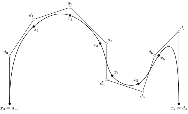
B-spline curve solving the above problem (see section 6.8). The next figure showsN+ 1 = 8 data points, and aC2_{-continuous spline curve} _F _{passing through these points, for a uniform}

sequence of reals ui.

Other pointsd₋1, . . . , d8 are also shown. What happens is that the interpolatingB-spline

curve is really determined by some sequence of points d₋1, . . . , dN+1 called de Boor control

points (with d₋₁ = x0 and dN+1 = xN). Instead of specifying the tangents at x0 and xN,

we can specify the control points d0 and dN. Then, it turns out that d1, . . . , dN−1 can be

computed fromx0, . . . , xN (and d0, dN) by solving a system of linear equations of the form

           1

α1 β1 γ1

α2 β2 γ2 0

. ..

0 αN−2 βN−2 γN−2

αN−1 βN−1 γN−1

1                       d0 d1 d2 .. .

dN−2

dN−1

dN            =            r0 r1 r2 .. .

rN−2

rN−1

rN           

wherer0 andrN may be chosen arbitrarily, the coefficientsαi, βi, γiare easily computed from

(20)

b

c

b

c

b

c

b

c

b

c

b

c

b

c

b

c

b

x0 =d−1

x1

x2

x3

x4

x5

x6

x7 =d8

d0

d1

d2

d3

d4

d5

d6

d7

Figure 1.1: A C2 _{interpolation spline curve passing through the points}_x

0, x1, x2, x3, x4, x5,

x6, x7

The previous example suggests that curves can be defined in terms of control points. Indeed, specifying curves and surfaces in terms of control points is one of the major techniques used in geometric design. For example, in medical imaging, one may want to find the contour of some organ, say the heart, given some discrete data. One may do this by fitting a B -spline curve through the data points. In computer animation, one may want to have a person move from one location to another, passing through some intermediate locations, in a smooth manner. Again, this problem can be solved using B-splines. Many manufacturing problems involve fitting a surface through some data points. Let us mention automobile design, plane design, (wings, fuselage, etc), engine parts, ship hulls, ski boots, etc.

(21)

Part I

Basics of Affine Geometry

(22)

(23)

Chapter 2 Basics of Affine Geometry

2.1 Affine Spaces

Geometrically, curves and surfaces are usually considered to be sets of points with some special properties, living in a space consisting of “points.” Typically, one is also interested in geometric properties invariant under certain transformations, for example, translations, rotations, projections, etc. One could model the space of points as a vector space, but this is not very satisfactory for a number of reasons. One reason is that the point corresponding to the zero vector (0), called the origin, plays a special role, when there is really no reason to have a privileged origin. Another reason is that certain notions, such as parallelism, are handled in an akward manner. But the deeper reason is that vector spaces and affine spaces really have different geometries. The geometric properties of a vector space are invariant under the group of bijective linear maps, whereas the geometric properties of an affine space are invariant under the group of bijective affine maps, and these two groups are not isomorphic. Roughly speaking, there are more affine maps than linear maps.

Affine spaces provide a better framework for doing geometry. In particular, it is possible to deal with points, curves, surfaces, etc, in an intrinsic manner, that is, independently of any specific choice of a coordinate system. As in physics, this is highly desirable to really understand what’s going on. Of course, coordinate systems have to be chosen to finally carry out computations, but one should learn to resist the temptation to resort to coordinate systems until it is really necessary.

Affine spaces are the right framework for dealing with motions, trajectories, and physical forces, among other things. Thus, affine geometry is crucial to a clean presentation of kinematics, dynamics, and other parts of physics (for example, elasticity). After all, a rigid motion is an affine map, but not a linear map in general. Also, given an m_×n matrix A

and a vectorb _∈Rm_{, the set}_U ₌_{_x_∈_Rn _| _Ax₌_b_}_{of solutions of the system} _Ax₌_b _{is an}

affine space, but not a vector space (linear space) in general.

(24)

Use coordinate systems only when needed!

This chapter proceeds as follows. We take advantage of the fact that almost every affine concept is the counterpart of some concept in linear algebra. We begin by defining affine spaces, stressing the physical interpretation of the definition in terms of points (particles) and vectors (forces). Corresponding to linear combinations of vectors, we define affine com-binations of points (barycenters), realizing that we are forced to restrict our attention to families of scalars adding up to 1. Corresponding to linear subspaces, we introduce affine subspaces as subsets closed under affine combinations. Then, we characterize affine sub-spaces in terms of certain vector sub-spaces called their directions. This allows us to define a clean notion of parallelism. Next, corresponding to linear independence and bases, we define affine independence and affine frames. We also define convexity. Corresponding to linear maps, we define affine maps as maps preserving affine combinations. We show that every affine map is completely defined by the image of one point and a linear map. We investi-gate briefly some simple affine maps, the translations and the central dilatations. Certain technical proofs and some complementary material on affine geometry are relegated to an appendix (see Chapter B).

Our presentation of affine geometry is far from being comprehensive, and it is biased towards the algorithmic geometry of curves and surfaces. For more details, the reader is referred to Pedoe [59], Snapper and Troyer [77], Berger [5, 6], Samuel [69], Tisseron [83], and Hilbert and Cohn-Vossen [42].

Suppose we have a particle moving in 3-space and that we want to describe the trajectory of this particle. If one looks up a good textbook on dynamics, such as Greenwood [40], one finds out that the particle is modeled as a point, and that the position of this point x

is determined with respect to a “frame” in R3 _{by a vector. Curiously, the notion of a}

frame is rarely defined precisely, but it is easy to infer that a frame is a pair (O,(−→e1,−→e2,−→e3))

consisting of an originO (which is a point) together with a basis of three vectors (−→e1,−→e2,−→e3).

For example, the standard frame inR3 _{has origin}_O _{= (0}_,₀_,_{0) and the basis of three vectors}

−→_e

1 = (1,0,0),−→e2 = (0,1,0), and −→e3 = (0,0,1). The position of a point xis then defined by

the “unique vector” from O tox.

But wait a minute, this definition seems to be defining frames and the position of a point without defining what a point is! Well, let us identify points with elements of R3_{. If so,}

given any two pointsa= (a1, a2, a3) andb = (b1, b2, b3), there is a uniquefree vector denoted

− →

ab froma to b, the vector −→ab= (b1−a1, b2−a2, b3−a3). Note that

b=a+−→ab,

addition being understood as addition in R3_{. Then, in the standard frame, given a point}

x = (x1, x2, x3), the position of x is the vector −→Ox = (x1, x2, x3), which coincides with the

(25)

2.1. AFFINE SPACES 15

b

c

b

c

b

c

O a

b

− →

ab

Figure 2.1: Points and free vectors

What if we pick a frame with a different origin, say Ω = (ω1, ω2, ω3), but the same basis

vectors (−→e1,−→e2,e−→3)? This time, the point x= (x1, x2, x3) is defined by two position vectors:

−→

Ox= (x1, x2, x3) in the frame (O,(−e→1,−→e2,−→e3)), and

−→

Ωx= (x1−ω1, x2−ω2, x3−ω3) in the frame (Ω,(−→e1,−→e2,−→e3)).

This is because

−→

Ox=−→OΩ +−→Ωx and O−→Ω = (ω1, ω2, ω3).

We note that in the second frame (Ω,(−→e1,−→e2,−→e3)), points and position vectors are no

longer identified. This gives us evidence that points are not vectors. It may be computation-ally convenient to deal with points using position vectors, but such a treatment is not frame invariant, which has undesirable effets. Inspired by physics, it is important to define points and properties of points that are frame invariant. An undesirable side-effect of the present approach shows up if we attempt to define linear combinations of points. First, let us review the notion of linear combination of vectors. Given two vectors −→u and −→v of coordinates (u1, u2, u3) and (v1, v2, v3) with respect to the basis (−→e1,−→e2,−→e3), for any two scalars λ, µ, we

can define the linear combination λ−→u +µ−→v as the vector of coordinates

(λu1+µv1, λu2+µv2, λu3+µv3).

If we choose a different basis (−→e′₁,−→e′₂,−→e′₃) and if the matrixP expressing the vectors (−→e′₁,−→e′₂,

−→

e′3) over the basis (−→e1,−→e2,−→e3) is

P =



aa12 bb12 cc12

a3 b3 c3

(26)

which means that the columns ofP are the coordinates of the−→e′_j over the basis (−→e1,−→e2,−→e3),

since

u1−→e1 +u2−→e2 +u3−→e3 =u′1

−→

e′₁ +u′₂−→e₂′ +u′₃−→e′₃ and v1−→e1 +v2−→e2 +v3−→e3 =v1′

−→

e′₁ +v′₂−→e₂′ +v₃′−→e′₃,

it is easy to see that the coordinates (u1, u2, u3) and (v1, v2, v3) of −→u and −→v with respect to

the basis (−→e1,−→e2,−→e3) are given in terms of the coordinates (u′1, u′2, u′3) and (v1′, v2′, v3′) of −→u

and −→v with respect to the basis (−→e′1,

−→

e′2,

−→

e′3) by the matrix equations

 uu12

u3

 =P

 u ′ 1 u′ 2 u′ 3   and  vv12

v3

 =P

 v ′ 1 v′ 2 v′ 3  .

From the above, we get

 u ′ 1 u′ 2

u′₃



=P−1

 uu12

u3   and  v ′ 1 v′ 2

v₃′



=P−1

 vv12

v3

 ,

and by linearity, the coordinates

(λu′₁+µv₁′, λu′₂+µv₂′, λu′₃+µv₃′) of λ−→u +µ−→v with respect to the basis (−→e′₁,−→e′₂,−→e′₃) are given by

 λu

′

1+µv1′

λu′

2+µv2′

λu′

3+µv3′



=λP−1

 uu12

u3



+µP−1

 vv12

v3



=P−1



λuλu12++µvµv12

λu3+µv3

 .

Everything worked out because the change of basis does not involve a change of origin. On the other hand, if we consider the change of frame from the frame (O,(−→e1,−→e2,−→e3)) to

the frame (Ω,(−→e1,−→e2,−→e3)), where −→OΩ = (ω1, ω2, ω3), given two points aand bof coordinates

(a1, a2, a3) and (b1, b2, b3) with respect to the frame (O,(−→e1,−→e2,−→e3)) and of coordinates

(a′

1, a′2, a′3) and (b′1, b′2, b′3) of with respect to the frame (Ω,(−→e1,−→e2,−→e3)), since

(a′1, a′2, a′3) = (a1−ω1, a2−ω2, a3−ω3) and (b′1, b′2, b′3) = (b1 −ω1, b2−ω2, b3−ω3),

the coordinates ofλa+µbwith respect to the frame (O,(−→e1,−→e2,−→e3)) are

(λa1+µb1, λa2+µb2, λa3+µb3),

but the coordinates

(27)

2.1. AFFINE SPACES 17 of λa+µb with respect to the frame (Ω,(−→e1,−→e2,−→e3)) are

(λa1+µb1−(λ+µ)ω1, λa2+µb2 −(λ+µ)ω2, λa3+µb3−(λ+µ)ω3)

which are different from

(λa1+µb1−ω1, λa2 +µb2−ω2, λa3+µb3−ω3),

unless λ+µ= 1.

Thus, we discovered a major difference between vectors and points: the notion of linear combination of vectors is basis independent, but the notion of linear combination of points is frame dependent. In order to salvage the notion of linear combination of points, some restriction is needed: the scalar coefficients must add up to 1.

A clean way to handle the problem of frame invariance and to deal with points in a more intrinsic manner is to make a clearer distinction between points and vectors. We duplicate

R3 _{into two copies, the first copy corresponding to points, where we forget the vector space}

structure, and the second copy corresponding to free vectors, where the vector space structure is important. Furthermore, we make explicit the important fact that the vector spaceR3 _acts

on the set of points R3_{: given any} _point _a _{= (}_a

1, a2, a3) and any vector −→v = (v1, v2, v3),

we obtain the point

a+−→v = (a1+v1, a2+v2, a3+v3),

which can be thought of as the result of translating a to b using the vector −→v . We can imagine that−→v is placed such that its origin coincides withaand that its tip coincides with

b. This action + : R3_×_R3 _→_R3 _{satisfies some crucial properties. For example,}

a+−→0 =a,

(a+−→u) +−→v =a+ (−→u +−→v ),

and for any two points a, b, there is a unique free vector −→ab such that

b=a+−→ab.

It turns out that the above properties, although trivial in the case of R3_{, are all that is}

needed to define the abstract notion of affine space (or affine structure). The basic idea is to consider two (distinct) sets E and −→E, where E is a set of points (with no structure) and

−→

(28)

For simplicity, it is assumed that all vector spaces under consideration are defined over the field R _{of real numbers. It is also assumed that all families of vectors and scalars are}

finite. The formal definition of an affine space is as follows.

Did you say “A fine space”?

Definition 2.1.1. An affine space is either the empty set, or a triple hE,−→E ,+i consisting of a nonempty set E (ofpoints), a vector space −→E (of translations, or free vectors), and an action + : E×−→E →E, satisfying the following conditions.

(AF1) a+ 0 =a, for every a∈E;

(AF2) (a+u) +v =a+ (u+v), for every a_∈E, and every u, v _∈−→E;

(AF3) For any two pointsa, b∈E, there is a uniqueu∈−→E such that a+u=b. The unique vector u_∈−→E such that a+u=b is denoted by−→ab, or sometimes by b₋a. Thus, we also write

b=a+−→ab

(or even b =a+ (b₋a)).

Thedimension of the affine spacehE,−→E ,+iis the dimension dim(−→E) of the vector space

−→_E_{. For simplicity, it is denoted as dim(}_E_).

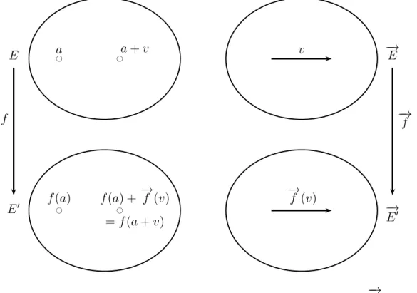
Note that _{−−−−−→}

a(a+v) = v

for alla∈Eand allv ∈−→E, since−−−−−→a(a+v) is the unique vector such thata+v =a+−−−−−→a(a+v). Thus, b = a+v is equivalent to −→ab = v. The following diagram gives an intuitive picture of an affine space. It is natural to think of all vectors as having the same origin, the null vector.

(29)

2.1. AFFINE SPACES 19

b

c

b

c

b

c

E −→E

a

b =a+u

c=a+w

u

v w

Figure 2.2: Intuitive picture of an affine space

For every a_∈E, consider the mapping from −→E to E:

u7→a+u,

where u∈−→E, and consider the mapping from E to−→E:

b_7→−→ab,

where b_∈E. The composition of the first mapping with the second is

u_7→a+u_7→−−−−−→a(a+u),

which, in view of (AF3), yields u. The composition of the second with the first mapping is

b7→−→ab7→a+−→ab,

which, in view of (AF3), yields b. Thus, these compositions are the identity from −→E to −→E

and the identity from E toE, and the mappings are both bijections.

When we identify E to −→E via the mapping b _7→ −→ab, we say that we consider E as the vector space obtained by taking a as the origin in E, and we denote it as Ea. Thus, an

affine space hE,−→E ,+i is a way of defining a vector space structure on a set of points E, without making a commitment to a fixed origin inE. Nevertheless, as soon as we commit to an origin a in E, we can view E as the vector space Ea. However, we urge the reader to

think of E as a physical set of points and of −→E as a set of forces acting on E, rather than reducingE to some isomorphic copy ofRn_{. After all, points are points, and not vectors! For}

notational simplicity, we will often denote an affine space _hE,−→E ,+_i as (E,−→E), or even as

(30)

One should be careful about the overloading of the addition symbol +. Addition is well-defined on vectors, as in u+v, the translate a+u of a point a_∈E by a vector u_∈−→E

is also well-defined, but addition of pointsa+b does not make sense. In this respect, the notation b−a for the unique vector u such that b =a+u, is somewhat confusing, since it suggests that points can be substracted (but not added!). Yet, we will see in section 10.1 that it is possible to make sense of linear combinations of points, and even mixed linear combinations of points and vectors.

Any vector space −→E has an affine space structure specified by choosing E = −→E, and letting + be addition in the vector space−→E. We will refer to this affine structure on a vector space as thecanonical (or natural) affine structure on −→E. In particular, the vector space Rn

can be viewed as an affine space denoted as An_{. In order to distinguish between the double}

role played by members of Rn_{, points and vectors, we will denote points as row vectors, and}

vectors as column vectors. Thus, the action of the vector space Rn _{over the set} _Rn _simply

viewed as a set of points, is given by

(a1, . . . , an) +

  

u1

.. .

un

 

= (a1+u1, . . . , an+un).

The affine space An _{is called the} _{real affine space of dimension} _n_{. In most cases, we will}

consider n = 1,2,3.

2.2 Examples of Affine Spaces

Let us now give an example of an affine space which is not given as a vector space (at least, not in an obvious fashion). Consider the subset L of A2 _{consisting of all points (}_{x, y}₎

satisfying the equation

x+y₋1 = 0.

The set Lis the line of slope ₋1 passing through the points (1,0) and (0,1).

The line Lcan be made into an official affine space by defining the action + : L_×R_→_L

of R _on_L _{defined such that for every point (}_x,₁₋_x_{) on} _L _{and any} _u_∈R_,

(x,1₋x) +u= (x+u,1₋x₋u).

It immediately verified that this action makes L into an affine space. For example, for any two points a = (a1,1−a1) and b = (b1,1−b1) on L, the unique (vector) u ∈ R such that

b =a+u is u=b1−a1. Note that the vector space Ris isomorphic to the line of equation

(31)

2.2. EXAMPLES OF AFFINE SPACES 21

b

c

b

c

L

Figure 2.3: An affine space: the line of equation x+y−1 = 0

Similarly, consider the subset H of A3 _{consisting of all points (}_{x, y, z}_{) satisfying the}

equation

x+y+z−1 = 0.

The set H is the plane passing through the points (1,0,0), (0,1,0), and (0,0,1). The plane

H can be made into an official affine space by defining the action + : H_×R2 _→_H _of _R2 _on

H defined such that for every point (x, y,1₋x₋y) onH and any

u v

∈R2_,

(x, y,1−x−y) +

u v

= (x+u, y+v,1−x−u−y−v).

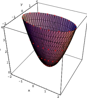
For a slightly wilder example, consider the subsetP ofA3 _{consisting of all points (}_{x, y, z}₎

satisfying the equation

x2+y2−z = 0.

The set P is paraboloid of revolution, with axis Oz. The surface P can be made into an official affine space by defining the action + : P ×R2 _→_P _of _R2 _on_P _{defined such that for}

every point (x, y, x2₊_y2_{) on} _P _{and any}

u v

∈R2_,

(x, y, x2₊_y2_{) +}

u v

= (x+u, y+v,(x+u)2_{+ (}_y₊_v₎2₎_.

(32)

b

c

b

c

b

c

E −→E

a

b

c

ab

bc ac

Figure 2.4: Points and corresponding vectors in affine geometry

2.3 Chasles’ Identity

Given any three points a, b, c∈E, sincec=a+−→ac, b =a+−→ab, and c=b+−→bc, we get

c=b+−→bc = (a+−→ab) +−→bc =a+ (−→ab+−→bc)

by (AF2), and thus, by (AF3),

− →

ab+−→bc =−→ac,

which is known as Chasles’ identity.

Since a=a+−→aa and by (AF1),a =a+ 0, by (AF3), we get

−→

aa = 0.

Thus, letting a=cin Chasles’ identity, we get

− →

ba =₋−→ab.

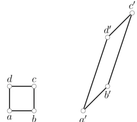
Given any four points a, b, c, d∈E, since by Chasles’ identity

− →

ab+−→bc =ad−→+−→dc=−→ac,

we have −→ab=−→dc iff −→bc =−ad→(the parallelogram law).

2.4 Affine Combinations, Barycenters

(33)

2.4. AFFINE COMBINATIONS, BARYCENTERS 23

b

c

b

c

b

c

b

c

O =d c

a

b

Figure 2.5: Two coordinates systems in R2

certain readers, we give another example showing what goes wrong if we are not careful in defining linear combinations of points. Consider R2 _{as an affine space, under its natural}

coordinate system with origin O = (0,0) and basis vectors

1 0

and

0 1

. Given any two

points a= (a1, a2) and b= (b1, b2), it is natural to define the affine combination λa+µb as

the point of coordinates (λa1+µb1, λa2+µb2).

Thus, when a= (₋1,₋1) and b= (2,2), the pointa+b is the point c= (1,1). However, let us now consider the new coordinate system with respect to the originc= (1,1) (and the same basis vectors). This time, the coordinates of a are (−2,−2), and the coordinates of b

are (1,1), and the point a+b is the point d of coordinates (−1,−1). However, it is clear that the point d is identical to the origin O = (0,0) of the first coordinate system. Thus,

a+b corresponds to two different points depending on which coordinate system is used for its computation!

Thus, some extra condition is needed in order for affine combinations to make sense. It turns out that if the scalars sum up to 1, the definition is intrinsic, as the following lemma shows.

Lemma 2.4.1. Given an affine space E, let (ai)i∈I be a family of points in E, and let

(λi)i∈I be a family of scalars. For any two points a, b∈E, the following properties hold: (1)

If P_i_∈_Iλi = 1, then

a+X

i∈I

λi−→aai =b+

X

i∈I

λi−→bai.

(2) If P_i_∈_Iλi = 0, then

X

i∈I

λi−→aai =

X

i∈I

(34)

Proof. (1) By Chasles’ identity (see section 2.3), we have

a+X

i∈I

λi−→aai =a+

X

i∈I

λi(−→ab+−→bai)

=a+ (X

i∈I

λi)−→ab+

X

i∈I

λi−→bai

=a+−→ab+X

i∈I

λi−→bai since P_i_∈_Iλi = 1

=b+X

i∈I

λi−→bai since b =a+−→ab.

(2) We also have

X

i∈I

λi−→aai =

X

i∈I

λi(−→ab+−→bai)

= (X

i∈I

λi)−→ab+

X

i∈I

λi−→bai

=X

i∈I

λi−→bai,

since P_i_∈_Iλi = 0.

Thus, by lemma 2.4.1, for any family of points (ai)i∈I in E, for any family (λi)i∈I of

scalars such that P_i_∈_Iλi = 1, the point

x=a+X

i∈I

λi−→aai

is independent of the choice of the origina_∈E. The unique point xis called the barycenter (or barycentric combination, or affine combination) of the points ai assigned the weights λi.

and it is denoted as _X

i∈I

λiai.

In dealing with barycenters, it is convenient to introduce the notion of a weighted point, which is just a pair (a, λ), wherea_∈E is a point, andλ _∈R_{is a scalar. Then, given a family}

of weighted points ((ai, λi))i∈I, where Pi∈I λi = 1, we also say that the point Pi∈Iλiai is

the barycenter of the family of weighted points ((ai, λi))i∈I. Note that the barycenter x of

the family of weighted points ((ai, λi))i∈I is the unique point such that

−→

ax=X

i∈I

(35)

2.4. AFFINE COMBINATIONS, BARYCENTERS 25 and setting a=x, the point x is the unique point such that

X

i∈I

λi−→xai = 0.

In physical terms, the barycenter is the center of mass of the family of weighted points ((ai, λi))i∈I (where the masses have been normalized, so that Pi∈Iλi = 1, and negative

masses are allowed).

Remarks:

(1) For all m ≥ 2, it is easy to prove that the barycenter of m weighted points can be obtained by repeated computations of barycenters of two weighted points.

(2) WhenP_i_∈_Iλi = 0, the vectorPi∈Iλi−→aai does not depend on the pointa, and we may

denote it asP_i_∈_Iλiai. This observation will be used in Chapter 10.1 to define a vector

space in which linear combinations of both points and vectors make sense, regardless of the value ofP_i_∈_Iλi.

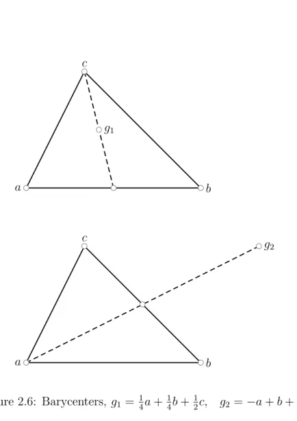
The figure below illustrates the geometric construction of the barycenters g1 and g2 of

the weighted points a,1 4

, b,1 4

, and c,1 2

, and (a,₋1), (b,1), and (c,1).

The point g1 can be constructed geometrically as the middle of the segment joining cto

the middle 1₂a+1₂b of the segment (a, b), since

g1 =

1 2

1 2a+

1 2b

+ 1 2c.

The point g2 can be constructed geometrically as the point such that the middle 1₂b+1₂c of

the segment (b, c) is the middle of the segment (a, g2), since

g2 =−a+ 2

1 2b+

1 2c

.

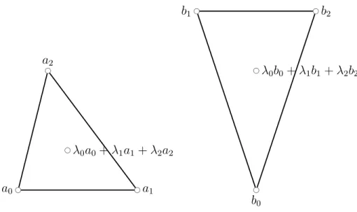
Later on, we will see that a polynomial curve can be defined as a set of barycenters of a fixed number of points. For example, let (a, b, c, d) be a sequence of points in A2_{. Observe}

that

(1−t)3+ 3t(1−t)2+ 3t2(1−t) +t3 = 1,

since the sum on the left-hand side is obtained by expanding (t+ (1₋t))3 _{= 1 using the}

binomial formula. Thus,

(1−t)3a+ 3t(1−t)2b+ 3t2(1−t)c+t3d

is a well-defined affine combination. Then, we can define the curve F: A_→A2 _{such that}

F(t) = (1₋t)3a+ 3t(1₋t)2b+ 3t2(1₋t)c+t3d.

(36)

b

c bc

b

c

b

c

b

c

b

c bc

b

c

b

c

b

c

a b

c

g1

a _b

c _g

2

(37)

2.5. AFFINE SUBSPACES 27

2.5 Affine Subspaces

In linear algebra, a (linear) subspace can be characterized as a nonempty subset of a vector space closed under linear combinations. In affine spaces, the notion corresponding to the notion of (linear) subspace is the notion of affine subspace. It is natural to define an affine subspace as a subset of an affine space closed under affine combinations.

Definition 2.5.1. Given an affine space _hE,−→E ,+_i, a subset V ofE is anaffine subspace if for every family of weighted points ((ai, λi))i∈I in V such that Pi∈Iλi = 1, the barycenter

P

i∈Iλiai belongs to V.

An affine subspace is also called a flat by some authors. According to definition 2.5.1, the empty set is trivially an affine subspace, and every intersection of affine subspaces is an affine subspace.

As an example, consider the subset U of A2 _{defined by}

U ={(x, y)∈R2 _| _ax₊_by ₌_c_}_,

i.e. the set of solutions of the equation

ax+by =c,

where it is assumed thata ₆= 0 orb₆= 0. Given any m points (xi, yi)∈U and any m scalars

λi such that λ1+· · ·+λm = 1, we claim that

m

X

i=1

λi(xi, yi)∈U.

Indeed, (xi, yi)∈U means that

axi+byi =c,

and if we multiply both sides of this equation by λi and add up the resulting m equations,

we get

m

X

i=1

(λiaxi +λibyi) = m

X

i=1

λic,

and since λ1+· · ·+λm = 1, we get

a

m

X

i=1

λixi

!

+b

m

X

i=1

λiyi

! = m X i=1 λi !

c=c,

which shows that

m

X

i=1

λixi, m

X

i=1

λiyi

!

=

m

X

i=1

(38)

Thus, U is an affine subspace ofA2_{. In fact, it is just a usual line in} _A2_.

It turns out that U is closely related to the subset of R2 _{defined by}

−→

U ={(x, y)∈R2 _| _ax₊_by _{= 0}_}_,

i.e. the set of solution of the homogeneous equation

ax+by= 0

obtained by setting the right-hand side of ax+by =cto zero. Indeed, for anym scalars λi,

the same calculation as above yields that

m

X

i=1

λi(xi, yi)∈−→U ,

this time without any restriction on the λi, since the right-hand side of the equation is

null. Thus, −→U is a subspace of R2_{. In fact,} −→_U _{is one-dimensional, and it is just a usual line}

in R2_{. This line can be identified with a line passing through the origin of} _A2_{, line which is}

parallel to the line U of equation ax+by = c. Now, if (x0, y0) is any point in U, we claim

that

U = (x0, y0) +−→U ,

where

(x0, y0) +−→U ={(x0+u1, y0+u2) | (u1, u2)∈−→U}.

First, (x0, y0) +−→U ⊆U, sinceax0+by0 =cand au1+bu2 = 0 for all (u1, u2)∈−→U. Second,

if (x, y)_∈U, then ax+by=c, and since we also have ax0+by0 =c, by subtraction, we get

a(x₋x0) +b(y−y0) = 0,

which shows that (x−x0, y−y0)∈−→U, and thus (x, y)∈(x0, y0) +−→U. Hence, we also have

U ⊆(x0, y0) +−→U, andU = (x0, y0) +−→U.

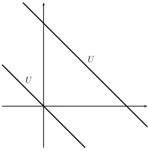
The above example shows that the affine line U defined by the equation

ax+by =c

is obtained by “translating” the parallel line −→U of equation

ax+by= 0

passing through the origin. In fact, given any point (x0, y0)∈U,

(39)

U

Figure 2.7: An affine line U and its direction

More generally, it is easy to prove the following fact. Given any m_×n matrix Aand any vector c∈Rm_{, the subset} _U _of _An _{defined by}

U ={x∈Rn _|_Ax ₌_c_}

is an affine subspace of An_{. Furthermore, if we consider the corresponding homogeneous}

equation Ax= 0, the set

−→

U =_{x_∈Rn

| Ax= 0_} is a subspace of Rn_{, and for any} _x

0 ∈U, we have

U =x0+−→U .

This is a general situation. Affine subspaces can be characterized in terms of subspaces of

−→

E. Let V be a nonempty subset of E. For every family (a1, . . . , an) in V, for any family

(λ1, . . . , λn) of scalars, for every point a∈V, observe that for every x∈E,

x=a+

n

X

i=1

λi−→aai

is the barycenter of the family of weighted points

((a1, λ1), . . . ,(an, λn),(a,1− n

X

i=1

(40)

since

n

X

i=1

λi+ (1− n

X

i=1

λi) = 1.

Given any point a_∈E and any subspace V of −→E, let a+V denote the following subset of E:

a+V =_{a+v _| v _∈V_}.

Lemma 2.5.2. LethE,−→E ,+ibe an affine space. (1) A nonempty subsetV ofE is an affine subspace iff, for every point a_∈V, the set

Va ={−ax→ | x∈V}

is a subspace of −→E. Consequently, V =a+Va. Furthermore,

V ={−xy→ | x, y ∈V}

is a subspace of −→E and Va=V for all a∈E. Thus, V =a+V.

(2) For any subspace V of −→E, for any a_∈E, the set V =a+V is an affine subspace.

Proof. (1) Clearly, −→0 ∈−→V . If V is an affine subspace, then V is closed under barycentric combinations, and by the remark before the lemma, for every x_∈E,

−→

ax=

n

X

i=1

λi−→aai

iff x is the barycenter

n

X

i=1

λiai + (1− n

X

i=1

λi)a

of the family of weighted points ((a1, λ1), . . . ,(an, λn),(a,1−Pn_i₌₁λi)). Then, it is clear

that Va is closed under linear combinations, and thus, it is a subspace of −→E. Since V =

{−xy→ _| x, y _∈V_} and Va = {−ax→ | x ∈ V}, where a ∈V, it is clear that Va ⊆V. Conversely,

since

−→

xy =−ay→_{− −}ax,→

and since Va is a subspace of−→E, we have V ⊆Va. Thus, V =Va, for every a∈V.

(2) IfV =a+V, whereV is a subspace of−→E, then, for every family of weighted points, ((a+vi, λi))1≤i≤n, wherevi ∈V, and λ1+· · ·+λn= 1, the barycenter x being given by

x=a+

n

X

i=1

λi−−−−−→a(a+vi) =a+ n

X

i=1

λivi

(41)

b

c

E −→E

a

V =a+V

V

Figure 2.8: An affine subspace V and its direction −→V

In particular, whenE is the natural affine space associated with a vector spaceE, lemma 2.5.2 shows that every affine subspace ofE is of the formu+U, for a subspace U ofE. The subspaces of E are the affine subspaces that contain 0.

The subspace V associated with an affine subspace V is called the direction of V. It is also clear that the map + : V _×V _→V induced by + : E_×−→E _→E confers to _hV, V,+_ian affine structure.

By the dimension of the subspace V, we mean the dimension of V. An affine subspace of dimension 1 is called a line, and an affine subspace of dimension 2 is called a plane. An affine subspace of codimension 1 is called a hyperplane (recall that a subspace F of a vector spaceE has codimension 1 iff there is some subspaceGof dimension 1 such thatE =F⊕G, the direct sum ofF andG, see Appendix A). We say that two affine subspaces U andV are parallel if their directions are identical. Equivalently, since U =V, we haveU =a+U, and

V =b+U, for any a∈U and any b∈V, and thus,V is obtained fromU by the translation

− →

ab.

By lemma 2.5.2, a line is specified by a point a ∈E and a nonzero vector v ∈−→E, i.e. a line is the set of all points of the form a+λu, for λ _∈ R_{. We say that three points} _{a, b, c}

are collinear, if the vectors −→ab and −→ac are linearly dependent. If two of the points a, b, c are distinct, say a ₆= b, then there is a unique λ _∈ R_{, such that} −→_ac ₌ _λ−→_ab_{, and we define the}

ratio −→ac

− →

ab =λ.

A plane is specified by a point a∈E and two linearly independent vectors u, v ∈−→E, i.e. a plane is the set of all points of the forma+λu+µv, for λ, µ_∈R_{. We say that four points}

a, b, c, dare coplanar, if the vectors −→ab,−→ac, and−→ad, are linearly dependent. Hyperplanes will be characterized a little later.

Lemma 2.5.3. Given an affine space _hE,−→E ,+_i, for any family (ai)i∈I of points in E, the

(42)

(ai)i∈I.

Proof. If (ai)i∈I is empty, then V = ∅, because of the condition P_i_∈_Iλi = 1. If (ai)i∈I is

nonempty, then the smallest affine subspace containing (ai)i∈I must contain the set V of

barycentersP_i_∈_Iλiai, and thus, it is enough to show thatV is closed under affine

combina-tions, which is immediately verified.

Given a nonempty subset S of E, the smallest affine subspace of E generated by S is often denoted as_hS_i. For example, a line specified by two distinct pointsa andb is denoted as ha, bi, or even (a, b), and similarly for planes, etc.

Remark: Since it can be shown that the barycenter of n weighted points can be obtained by repeated computations of barycenters of two weighted points, a nonempty subset V of

E is an affine subspace iff for every two points a, b ∈ V, the set V contains all barycentric combinations of aand b. IfV contains at least two points,V is an affine subspace iff for any two distinct points a, b_∈V, the set V contains the line determined by a and b, that is, the set of all points (1−λ)a+λb, λ∈R_.

2.6 Affine Independence and Affine Frames

Corresponding to the notion of linear independence in vector spaces, we have the notion of affine independence. Given a family (ai)i∈I of points in an affine spaceE, we will reduce the

notion of (affine) independence of these points to the (linear) independence of the families (−−→aiaj)j∈(I−{i}) of vectors obtained by chosing any ai as an origin. First, the following lemma

shows that it sufficient to consider only one of these families.

Lemma 2.6.1. Given an affine space _hE,−→E ,+_i, let (ai)i∈I be a family of points in E. If

the family (−−→aiaj)j∈(I−{i}) is linearly independent for somei∈I, then(−−→aiaj)j∈(I−{i}) is linearly

independent for every i∈I.

Proof. Assume that the family (−−→aiaj)j∈(I−{i}) is linearly independent for some specific i∈I.

Let k∈I with k 6=i, and assume that there are some scalars (λj)j∈(I−{k}) such that

X

j∈(I−{k})

λj−−→akaj =−→0 .

Since

−−→

(43)

2.6. AFFINE INDEPENDENCE AND AFFINE FRAMES 33 we have

X

j∈(I−{k})

λj−−→akaj =

X

j∈(I−{k})

λj−−→akai+

X

j∈(I−{k})

λj−−→aiaj,

= X

j∈(I−{k})

λj−−→akai+

X

j∈(I−{i,k})

λj−−→aiaj,

= X

j∈(I−{i,k})

λj−−→aiaj −

  X

j∈(I−{k})

λj

 −−→aiak,

and thus

X

j∈(I−{i,k})

λj−−→aiaj −

  X

j∈(I−{k})

λj



−−→aiak=−→0.

Since the family (−−→aiaj)j∈(I−{i}) is linearly independent, we must have λj = 0 for all j ∈

(I_{− {}i, k_}) andP_j_∈₍_I_−{_k_}₎λj = 0, which implies that λj = 0 for allj ∈(I− {k}).

We define affine independence as follows.

Definition 2.6.2. Given an affine spacehE,−→E ,+i, a family (ai)i∈I of points inE isaffinely

independent if the family (−−→aiaj)j∈(I−{i}) is linearly independent for some i∈I.

Definition 2.6.2 is reasonable, since by Lemma 2.6.1, the independence of the family (−−→aiaj)j∈(I−{i}) does not depend on the choice ofai. A crucial property of linearly independent

vectors (−→u1, . . . ,−→um) is that if a vector −→v is a linear combination

−→_v ₌Xm

i=1

λi−→ui

of the −→ui, then the λi are unique. A similar result holds for affinely independent points.

Lemma 2.6.3. Given an affine spacehE,−→E ,+i, let (a0, . . . , am) be a family of m+ 1 points

in E. Let x ∈ E, and assume that x = Pm_i₌₀λiai, where Pmi=0λi = 1. Then, the family

(λ0, . . . , λm) such that x = Pm_i₌₀λiai is unique iff the family (−−→a0a1, . . . ,−−→a0am) is linearly

independent.

Proof. Recall that

x=

m

X

i=0

λiai iff −→a0x=

m

X

i=1

λi−−→a0ai,

where Pm_i₌₀λi = 1. However, it is a well known result of linear algebra that the family

(λ1, . . . , λm) such that

−→

a0x=

m

X

i=1

(44)

b

c

b

c

b

c

E −→E

a0 a1

a2

a0a1

a0a2

Figure 2.9: Affine independence and linear independence

is unique iff (−−→a0a1, . . . ,−−→a0am) is linearly independent (for a proof, see Chapter A, Lemma

A.1.10). Thus, if (−−→a0a1, . . . ,−−→a0am) is linearly independent, by lemma A.1.10, (λ1, . . . , λm)

is unique, and since λ0 = 1− Pm_i₌₁λi, λ0 is also unique. Conversely, the uniqueness of

(λ0, . . . , λm) such thatx=Pmi=0λiai implies the uniqueness of (λ1, . . . , λm) such that

−→

a0x=

m

X

i=1

λi−−→a0ai,

and by lemma A.1.10 again, (−−→a0a1, . . . ,−−→a0am) is linearly independent.

Lemma 2.6.3 suggests the notion of affine frame. Affine frames are the affine analogs of bases in vector spaces. Let hE,−→E ,+i be a nonempty affine space, and let (a0, . . . , am)

be a family of m + 1 points in E. The family (a0, . . . , am) determines the family of m

vectors (−−→a0a1, . . . ,−−→a0am) in −→E. Conversely, given a point a0 in E and a family of m vectors

(u1, . . . , um) in−→E, we obtain the family ofm+ 1 points (a0, . . . , am) inE, whereai =a0+ui,

1≤i≤m.

Thus, for any m≥1, it is equivalent to consider a family of m+ 1 points (a0, . . . , am) in

E, and a pair (a0,(u1, . . . , um)), where the ui are vectors in −→E.

When (−−→a0a1, . . . ,−−→a0am) is a basis of −→E, then, for every x∈E, since x =a0+−→a0x, there

is a unique family (x1, . . . , xm) of scalars, such that

x=a0+x1−−→a0a1+· · ·+xm−−→a0am.

The scalars (x1, . . . , xm) are coordinates with respect to (a0,(a−−→0a1, . . . ,−−→a0am)). Since

x=a0+

m

X

i=1

xi−−→a0ai iff x= (1− m

X

i=1

xi)a0+

m

X

i=1

(45)

2.6. AFFINE INDEPENDENCE AND AFFINE FRAMES 35

x∈E can also be expressed uniquely as

x=

m

X

i=0

λiai

with Pm_i₌₀λi = 1, and where λ0 = 1−Pmi=1xi, and λi = xi for 1 ≤ i ≤ m. The scalars

(λ0, . . . , λm) are also certain kinds of coordinates with respect to (a0, . . . , am). All this is

summarized in the following definition.

Definition 2.6.4. Given an affine space hE,−→E ,+i, an affine frame with origin a0 is a

family (a0, . . . , am) ofm+ 1 points inE such that (−−→a0a1, . . . ,−−→a0am) is a basis of −→E. The pair

(a0,(−−→a0a1, . . . ,a−−→0am)) is also called an affine frame with origina0. Then, everyx∈E can be

expressed as

x=a0+x1−−→a0a1+· · ·+xm−−→a0am

for a unique family (x1, . . . , xm) of scalars, called the coordinates ofx w.r.t. the affine frame

(a0,(−−→a0a1, . . . ,−−→a0am)). Furthermore, every x∈E can be written as

x=λ0a0+· · ·+λmam

for some unique family (λ0, . . . , λm) of scalars such thatλ0+· · ·+λm = 1 called thebarycentric

coordinates of x with respect to the affine frame (a0, . . . , am).

The coordinates (x1, . . . , xm) and the barycentric coordinates (λ0, . . . , λm) are related by

the equations λ0 = 1−Pmi=1xi and λi = xi, for 1 ≤ i ≤ m. An affine frame is called an

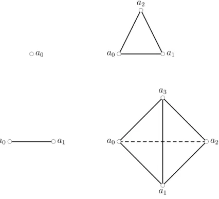
affine basis by some authors. The figure below shows affine frames for_|I_|= 0,1,2,3.

A family of two points (a, b) inE is affinely independent iff−→ab 6= 0, iffa6=b. Ifa 6=b, the affine subspace generated byaand bis the set of all points (1₋λ)a+λb, which is the unique line passing through a and b. A family of three points (a, b, c) in E is affinely independent iff −→ab and −→ac are linearly independent, which means that a, b, and c are not on a same line (they are not collinear). In this case, the affine subspace generated by (a, b, c) is the set of all points (1₋λ₋µ)a+λb+µc, which is the unique plane containing a, b, and c. A family of four points (a, b, c, d) in E is affinely independent iff−→ab, −→ac, and−→ad are linearly independent, which means that a, b, c, and d are not in a same plane (they are not coplanar). In this case, a, b, c, and d, are the vertices of a tetrahedron.

Givenn+1 affinely independent points (a0, . . . , an) inE, we can consider the set of points

λ0a0+· · ·+λnan, whereλ0+· · ·+λn= 1 andλi ≥0 (λi ∈R). Such affine combinations are

called convex combinations. This set is called the convex hull of (a0, . . . , an) (or n-simplex

spanned by (a0, . . . , an)). When n = 1, we get the line segment between a0 anda1, including

a0 and a1. When n = 2, we get the interior of the triangle whose vertices are a0, a1, a2,

including boundary points (the edges). When n= 3, we get the interior of the tetrahedron whose vertices are a0, a1, a2, a3, including boundary points (faces and edges). The set

Curves and Surfaces in Geometric Modeling: Theory & Algorithms - Free Computer, Programming, Mathematics, Technical Books, Lecture Notes and Tutorials