Lagrangian Heuristics for Large-Scale
Dynamic Facility Location with Generalized
Modular Capacities
Sanjay Dominik Jena
Centre interuniversitaire de recherche sur les r´eseaux d’entreprise, la logistique et le transport (CIRRELT), D´epartement d’informatique et de recherche op´erationnelle, Universit´e de Montr´eal
Jean-Fran¸cois Cordeau
Centre interuniversitaire de recherche sur les r´eseaux d’entreprise, la logistique et le transport (CIRRELT), Canada Research Chair in Logistics and Transportation, HEC Montr´eal
Bernard Gendron
Centre interuniversitaire de recherche sur les r´eseaux d’entreprise, la logistique et le transport (CIRRELT), D´epartement d’informatique et de recherche op´erationnelle, Universit´e de Montr´eal
Abstract
We consider the Dynamic Facility Location Problem with Generalized Modular Capacities,
a multi-period facility location problem in which the costs for capacity changes may differ for
all pairs of capacity levels. The problem embeds a complex cost structure and generalizes several existing facility location problems, such as those that allow temporary facility closing
or capacity expansion and reduction. As the model may become very large, general-purpose
mixed-integer programming (MIP) solvers are limited to solving instances of small to medium
size. In this paper, we extend the generalized model to the case of multiple commodities. We propose Lagrangian heuristics, based on subgradient and bundle methods, to find good quality
solutions for large-scale instances with up to 250 facility locations and 1,000 customers. To
improve the final solution quality, a restricted MIP model is solved based on the information
collected through the solution of the Lagrangian dual. Computational results show that the Lagrangian based heuristics provide highly reliable results for all problem variants considered.
They produce good quality solutions in short computing times even for instances where
state-of-the-art MIP solvers do not find feasible solutions. The strength of the formulation also allows
1
Introduction
Capacitated dynamic facility location problems typically aim at providing capacity planning over a
multiple-period planning horizon. Given that customer demands may vary significantly over time,
facilities often adjust their capacities. These problems find applications in both the public and private sectors, for the location of production facilities (Fleischmann et al., 2006), schools (Peeters
and Antunes, 2001), health care facilities (Correia and Captivo, 2003; Kim and Kim, 2013) and
many more, as documented in several recent literature surveys (Thomas and Griffin, 1996; Brotcorne et al., 2003; Revelle et al., 2008; Melo et al., 2009; Smith et al., 2009). To allow the adjustment
of capacities in such problems, common actions include capacity expansion and reduction (Luss,
1982; Jacobsen, 1990; Peeters and Antunes, 2001; Troncoso and Garrido, 2005; Dias et al., 2007), temporary closing of facilities (Chardaire and Sutter, 1996; Canel et al., 2001; Dias et al., 2006) and
the relocation of facilities (Melo et al., 2006). Although mathematical models often take into account
complex environments such as complete supply chains, the cost structure to adjust capacities along time is commonly modeled in less detail. Economies of scale are often represented on the level of
the total capacity involved in each operation, but do not take into consideration the capacity level
before the change. A more detailed representation of the cost structure is necessary in a number of applications, especially in the fields of transportation, logistics and telecommunications, where
additional capacity gets cheaper (or more expensive) when approaching the maximum capacity
limit. For instance, in the problem introduced by Jena et al. (2015b), logging camps are located to host workers in the forest industry. In this problem, the total capacity of a camp is represented
by its number of different hosting units, while additional units provide supporting infrastructure. As the relation between the number of different units cannot be captured by a simple function, the
costs for capacity changes need to be described by a cost matrix.
Jena et al. (2015a) recently introduced the Dynamic Facility Location Problem with Generalized Modular Capacities (DFLPG), in which the costs for capacity changes are based on a cost matrix.
The mixed-integer programming (MIP) model presented by the authors therefore allows taking
into account not only the total capacity involved in the capacity change, but also the current capacity level. This model generalizes several multi-period facility location problems: the problem
with facility closing and reopening, the problem with capacity expansion and reduction, and the
combination of both. In addition, the DLFPG formulation provides a strong linear programming (LP) relaxation bound. Compared to alternative MIP formulations, the DFLPG based models can
often be solved twice as fast using a general-purpose MIP solver. Although it is possible to solve the
models for small and medium size instances, they usually become too large when considering more complex problem variants or larger instances. In this case, heuristics are interesting alternatives.
Metaheuristics such as tabu search, simulated annealing and genetic algorithms have been
frequently applied to several families of location problems, from classical facility location problems (Arostegui et al., 2006) to logistics network design that model entire supply chains (Lee and Dong,
2008; Melo et al., 2011). Lagrangian relaxation based heuristics have been developed for several
1993; Sridharan, 1995; Holmberg and Ling, 1997; Agar and Salhi, 1998; Holmberg and Yuan, 2000;
Correia and Captivo, 2003; Wu et al., 2006), some of which combined Langrangian relaxation and local search (Correia and Captivo, 2006; Hinojosa et al., 2008; Li et al., 2009). Lagrangian bounds
have also been used within exact methods (G¨ortz and Klose, 2012). For multi-period facility
location, approaches based on Lagrangian relaxation have been proposed for problems without capacities (Chardaire and Sutter, 1996), with fixed capacities (Shulman, 1991), and for
multi-echelon problems in the context of supply chain design (Hinojosa et al., 2000; Diabat et al., 2011).
Furthermore, Lagrangian based methods have been successfully applied to other location problems such as dynamic hub location (Elhedhli and Wu, 2010; Contreras et al., 2011).
In this paper, we present an extension of the DFLPG in which customers have demands for
multiple commodities. We propose Lagrangian based heuristics that find good quality solutions in reasonable computing times. Two methods are introduced to solve the Lagrangian dual: a
subgra-dient method and a bundle method. After this process, a second optimization step is performed to improve the solution quality. This step consists of solving a restricted MIP model, taking into
consideration only decisions that have been part of a significant number of the previous Lagrangian
solutions. To the best of our knowledge, this work is the first to present a Lagrangian relaxation approach to solve large-scale instances of a multi-period facility location problem of this nature,
i.e., including modular capacity levels and multiple commodities. Very recently, the methodology
introduced here has been adapted to handle a more complex location problem from the forest industry (Jena et al., 2016). Given the strength of the formulation used to model the DFLPG,
the here presented Lagrangian heuristics are capable of providing relatively tight bounds on the
optimal solution value. The results are stable even for large instances, where general-purpose MIP solvers either consume too much memory or do not solve the problem in reasonable time. Further,
the proposed heuristic can handle an entire class of problems, consisting of all those that can be
modeled by the DFLPG.
The remainder of the paper is organized as follows. Section 2 reviews and extends the MIP
formulation for the DFLPG and shows how it can be used to model three different special cases.
Section 3 explains how the problem is decomposed via Lagrangian relaxation and outlines the resulting heuristics. Section 4 then discusses how the final solution quality can be improved in a
second optimization phase, using information from the solution of the Lagrangian dual to generate
a restricted MIP model. The Lagrangian heuristics are then compared by means of computational experiments in Section 5. First, general results are presented for each of the different problem
variants. Then, the advantages of the Lagrangian heuristics are illustrated with more detailed
results comparing their performance to a state-of-the-art MIP solver. Finally, conclusions are drawn in Section 6.
2
Mixed Integer Programming Formulation
This section first introduces a general formulation for the DFLPG and then explains how it can
introduced by Jena et al. (2015a) and extend it to include multiple commodities. We denote by
J the set of candidate facility locations and byL={0,1, . . . , q} the set of possible capacity levels for each facility. We also denote by I the set of customer demand points and by T the set of
time periods in the planning horizon. Without loss of generality, we assume throughout that the
beginning of periodt+ 1 corresponds to the end of period t. In addition, we make the assumption that all facility openings, closings and capacity changes are implemented at the beginning of a
time period. We denote by P the set of different commodities. The demand of customer i for commodity p in period t is denoted bydt
ip, while the cost to serve one unit of commodity p from
facilityjoperating at capacity level`to customeriduring periodtis denoted bygi`pjt . The capacity of a facility of size `at location j is given by uj` (withuj0 = 0). The cost matrixf``jt0 describes the combined cost to change the capacity level of a facility at locationj from` to`0 at the beginning of period t and to operate the facility at capacity level`0 throughout time period t. Furthermore, we let `j be the initial capacity level of an existing facility at locationj.
To formulate the problem, we use binary variables y``jt0 equal to 1 if and only if the facility at location j changes its capacity level from ` to `0 at the beginning of period t. Depending on the application context, only a limited set of capacity changes may be eligible in practice. To explicitly model those restrictions, we use the following two sets defining the eligible capacity changes. For
a facility j open at capacity level `, we define L−(j, t, `)⊆L as the set of capacity levels to which the capacity may be changed at the beginning of period t. The other way around, we define
L+(j, t, `) ⊆ L as the set of capacity levels from which the capacity may be changed to level `
at facility j at the beginning of period t. The allocation variables xjti`p denote the fraction of the demand of customer ifor commodity pin period tthat is served from a facility of size`located at
j. Using this notation, we define the following MIP model, referred to as theGeneralized Modular Capacities (GMC) formulation:
(GMC) minX
j∈J
X
t∈T
X
`∈L
X
`0∈L−(j,t,`)
f``jt0y``jt0+
X
i∈I
X
j∈J
X
`∈L
X
p∈P
X
t∈T
gi`pjt dtipxjti`p (1)
s.t. X
j∈J
X
`∈L
xjti`p= 1 ∀i∈I, ∀p∈P, ∀t∈T (2)
X
i∈I
X
p∈P
dtipxjti`p≤ X
`0∈L+(j,t,`)
uj`y`jt0` ∀j∈J, ∀`∈L, ∀t∈T (3)
xjti`p ≤`0∈L+(j, t, `)y`jt0` ∀i∈I, ∀j∈J, ∀`∈L, ∀p∈P, ∀t∈T. (4)
X
`0∈L+(j,t−1,`)
y`j0(`t−1)=
X
`0∈L−(j,t,`)
y``jt0 ∀j∈J, ∀`∈L, ∀t∈T\ {1} (5)
X
`∈L−(j,t,`j)
yj`j1`= 1 ∀j ∈J (6)
xjti`p ≥0 ∀i∈I, ∀j∈J, ∀`∈L, ∀p∈P, ∀t∈T (7)
The objective function (1) minimizes the total cost for changing the capacity levels and serving
the demand. Constraints (2) are the demand constraints for the customers. Constraints (3) are the capacity constraints at the facilities. Constraints (4), called Strong Inequalities (SIs), ensure that no demand can be served from a facility of sizelat periodtif no such facility is available at period
t. Since the capacity constraints are also enforcing the same requirements, the SIs are redundant for the MIP model, but they strengthen the LP relaxation bound. Similar inequalities, which can
be seen as a special case of flow cover inequalities (Padberg et al., 1983), are used in many facility location and network design problems (e.g., Gendron, 2011; Chouman et al., 2016) Constraints (5)
link the capacity change variables in consecutive time periods. Constraints (6) initialize the sizes
of the facilities at the beginning of the planning horizon, ensuring that exactly one capacity level is selected. Note that the we assume that all commodities are measured in the same units. If the
commodities consume different amounts of production capacity, the term dtipxjti`p can be replaced by dtipvpxjti`p. In this case, vp is the unit consumption factor of commodity p, i.e., the quantity of
capacity consumed to produce one unit of commodity p.
While constraints (2) and (3) define a transportation network typically found in facility location
problems, flow constraints (5) and (6) define, for each facility j ∈ J, an additional network that represents the evolution of the capacity of facilityj over time. In this acyclic network, nodes are
given by pairs< `, t > and arcs y``jt0 represent feasible binary capacity changes from node < `, t > to node < `0, t+ 1>. The network structure allows for a flexible representation of the underlying application, since feasible capacity changes and their corresponding costs can be defined differently
for each facility, time period and pair of capacity levels.
Special Cases. By careful design of the problem’s network structure, i.e., the definition of
feasible capacity level nodes and capacity change arcs, several variants of the problem can be
modeled as special cases of the GMC formulation. In this paper, three of them will be considered:
1. Dynamic Modular Capacitated Facility Location Problem with Closing and Reopening (DM-CFLP CR). In this problem, the size of a facility is chosen from a discrete set of capacity levels. Existing facilities may then be closed and reopened several times.
2. Dynamic Modular Capacitated Facility Location Problem with Capacity Expansion and Re-duction (DMCFLP ER). In this problem, the size of a facility is first chosen from a discrete set of capacity levels. Then, its capacity may be expanded or reduced from one capacity level
to another at each subsequent time period.
3. Dynamic Modular Capacitated Facility Location Problem with Closing/Reopening and Capac-ity Expansion/Reduction (DMCFLP CR ER). This problem allows for all operations defined in the previous two problems: facility closing and reopening, as well as the capacity expansion and reduction at existing facilities.
Each of these problems can be modeled using the GMC formulation by selecting a subset of
A detailed description can be found in the online Appendix A.
3
Lagrangian Relaxation
When applying Lagrangian relaxation to capacitated facility location problems, a promising and
popular choice (e.g., Shulman, 1991; Beasley, 1993; Hinojosa et al., 2000; Wu et al., 2006) is to relax the demand constraints, which yields a Lagrangian subproblem that can be solved efficiently. Let
α be the vector of Lagrange multipliers associated with the demand constraints (2). After relaxing
these constraints and rearranging the terms in the objective function, we obtain the following Lagrangian subproblem:
L(α) = minX
j∈J
X
`∈L
X
`0∈L−(j,t,`)
X
t∈T
f``jt0y
jt ``0
+X
i∈I
X
j∈J
X
`∈L
X
p∈P
X
t∈T
(gjti`pdtip−αtip)xjti`p+X
i∈I
X
p∈P
X
t∈T
αtip
s.t. (3)−(8).
3.1 Solution of the Lagrangian Subproblem
Let ˜cjti`p=gjti`pdipt −αtipdenote the modified costs for thexjti`pvariables. We separate the Lagrangian subproblem into |J|independent subproblems, one for each candidate facility location for a fixed
set of Lagrange multipliers α. The Lagrangian subproblem is solved as L(α) = P
j∈JLj(α) +
P
i∈I
P
p∈P
P
t∈Tαtip, where Lj(α) is defined as follows:
Lj(α) = min
X
`∈L
X
`0∈L−(j,t,`)
X
t∈T
f``jt0y``jt0+
X
i∈I
X
`∈L
X
p∈P
X
t∈T
˜
cjti`pxjti`p
s.t. X
i∈I
X
p∈P
dtipxjti`p≤ X
`0∈L+(j,t,`)
uj`yjt`0` ∀`∈L, ∀t∈T
X
`0∈L+(j,t−1,`)
y`j0(`t−1) =
X
`0∈L−(j,t,`)
y``jt0 ∀`∈L, ∀t∈T\ {1}
X
`∈L−(j,t,`j)
y`jj1` = 1
xjti`p≤ X
`0∈L+(j,t,`)
y`jt0` ∀i∈I, ∀`∈L, ∀p∈P, ∀t∈T
xjti`p≥0 ∀i∈I, ∀`∈L, ∀p∈P, ∀t∈T
y``jt0 ∈ {0,1} ∀`∈L, ∀`0 ∈L−(j, t, `), ∀t∈T.
Each of these subproblems (one for each location j ∈J) is concerned with finding the optimal
capacity planning over time, i.e., an optimal schedule for changing the facility capacities such
optimal demand allocation at capacity level `and period tcan be efficiently computed by solving
a continuous knapsack problem. This is done by rearranging the demand nodes dtip in increasing
order of their ratio of adjusted transportation costs and demand quantity, i.e., ˜c jt i`p
dtip, and by serving
demands until either the entire capacity uj` is filled or a demand node with a positive adjusted transportation cost is met. Once the optimal demand allocation costs are computed for each
possible capacity level decision, the Lagrangian subproblem can be solved separately for each facility by computing the shortest path in the acyclic capacity change network structure, for example by
adapting the dynamic programming approach presented by Shulman (1991).
Note that, without the use of the SIs, the Lagrangian subproblem does not possess the integral-ity property (Geoffrion, 1974), since facilintegral-ity capacities will only be opened as much as forced by
the capacity constraints, i.e., P
`0∈L+(j,t,`)y
jt `0` =
P
i∈I
P
p∈P(dtipx jt i`p)/u
j
`, which may be fractional.
Adding the SIs to the problem strengthens the dependence between the opening decisions and the demand allocation: P
`0∈L+(j,t,`)y`jt0`≥maxi∈I,p∈P{xjti`p}. The variablesxjti`p(and therefore also one
of the corresponding yjt`0` variables) will take value 1 if their modified costs ˜c
jt
i`p compensate the
costs for the open facility. As a consequence, using the SIs, the Lagrangian subproblem also has the integrality property. The lower bound provided by the Lagrangian dual will therefore never be
better than the bound provided by the LP relaxation of the original problem using the SIs.
3.2 Solution of the Lagrangian Dual
The solution of the Lagrangian subproblem, for any choice of the Lagrange multipliersα, provides a lower bound to the DFLPG. To obtain the best possible lower bound, one must solve the Lagrangian
dual:
z∗ = max
α L(α).
The Lagrangian function L(α) is non-differentiable. However, a subgradient direction can be
easily computed. We consider two different methods to solve the Lagrangian dual: a subgradient method and a bundle method.
Subgradient Method. The subgradient direction γipkt at the kth iteration is computed as the violation of the relaxed constraints whenx is fixed to the values found by solving the Lagrangian
subproblem:
γipkt= 1−X
j∈J
X
`∈L
xjti`p ∀i∈I, ∀p∈P, ∀t∈T.
other works (Shulman, 1991; Sridharan, 1991; Correia and Captivo, 2003):
λk=δk Zb−L
k(α)
P
i∈I
P
p∈P
P
t∈T(γipkt)2
,
where δk is a scalar, Lk(α) equals the value of L(α) at iteration k and Zb is the cost of the best
feasible solution found so far. The Lagrange multipliers for the (k+ 1)th iteration are then updated by:
αip(k+1)t=αktip+λkγipkt ∀i∈I, ∀p∈P, ∀t∈T.
Bundle Method. The second method used to solve the Langrangian dual is an implementation
of the aggregated bundle method (Frangioni, 2005). The method uses a subset of the tuples
< L(αs), γs >with s∈B, where B is referred to as the bundle of subgradientsγs, and αs is the corresponding vector of multipliers. From the primal viewpoint, the following quadratic problem
has to be solved at each iteration (Frangioni and Gallo, 1999):
min
θs
(
1 2 k
X
s∈B
γsθs k2+1
REBθ; s.t.
X
s∈B
θs = 1, θ≥0
)
,
where R is the so-called trust region, and Es =L(α) +γ( ˆα−α)−L( ˆα) is the linearization error
from the current point ˆα. The solution values forθs, given for each bundle member, hold valuable information and can be used to construct feasible integer solutions (see Section 4.2). The tentative ascent direction is then computed by the convex combination of the subgradients, using the convex
multipliers θ. Alternatively, the dual problem can be solved to compute the ascent direction, or directly the new point. Frangioni and Gallo (1999) elaborate on this relationship in detail.
Bundle methods usually possess stronger convergence properties than subgradient methods.
However, they also tend to require more time to compute the Lagrange multipliers. They are therefore beneficial when a small number of iterations is performed to reach the desired accuracy.
When the subproblem is block separable, disaggregated bundle methods (e.g., Frangioni and
Gorgone, 2014) may lead to stronger convergence than aggregated methods. While aggregated bundle methods use one set of subgradients for the entire subproblem, disaggregated methods use
one set of subgradients for each block of the subproblem. However, the computational costs and
memory requirements may be significantly higher than for an aggregated version. Even though disaggregated methods have been found to be very efficient for several problems, they did not lead
to competitive results for our problems (see Section 5.2). We therefore do not further elaborate on
their details.
3.3 Upper Bound Generation
At each iteration, a feasible solution is generated based on the Lagrangian solution obtained by
inte-ger solution of the problem that directly impacts the convergence of the subgradient and bundle
methods. Even though high quality upper bounds are desirable, it is important that they are gen-erated in an efficient manner, as the solution of the Lagrangian dual typically involves hundreds of
iterations.
The solution of the Lagrangian subproblem provides a facility opening schedule for the entire planning horizon. This schedule is defined by capacity levels `(j, t) indicating the facility size at
locationj at time periodt. In addition to the schedule, the Lagrangian solution provides a demand
allocation. As the demand constraints (2) have been relaxed, the customer demands dtip are either exactly met, under-served or over-served.
The set of all customer demands can therefore be separated into three subsets, where Σ1, Σ2
and Σ3 denote the demands defined by triplets< i, p, t >, which are exactly met, over-served and under served, respectively:
Σ1=
< i, p, t >:X
j∈J
xjt
i`(j,t)p = 1
,Σ2=
< i, p, t >:X
j∈J
xjt
i`(j,t)p>1
and Σ3 =
< i, p, t >:X
j∈J
xjt
i`(j,t)p <1
.
To obtain an integer feasible solution, we heuristically reduce redundant demand allocations for the pairs in Σ2 and increase missing demand allocations for the pairs in Σ3. Then, we heuristically
increase the available capacity to meet the missing demand. The heuristic procedure used to obtain
a feasible solution comprises the following steps:
1. Reduce demand allocation: For each < i, p, t >∈Σ2, all facility/size pairs (j, `(j, t)) are sorted in decreasing order of their allocation costs gjti`p. The allocated flow is removed until the total allocated demand for < i, p, t >equals 1.
2. Increase capacities: If the total remaining capacity is smaller than the total remaining
demand, we increase the capacity sequentially for each time period according to the following steps until the total demand can be met. Facilities are considered without a specific order.
We consider two simple possibilities to increase capacity: if a facility is already open at
any moment in the planning horizon, its capacity level at the current time period is set to maxt=1,···,|T|
n
`(j, t)o, i.e., the facility’s highest capacity level throughout the planning
horizon; if no facility exists, we increase the capacity level until the missing capacity is
covered or the maximum capacity level for this facility is reached.
3. Increase the demand allocation: For each< i, p, t >∈Σ3, all facility/size pairs (j, `(j, t)) with remaining capacity are sorted in increasing order of their allocation costsgjti`p. Demand is allocated to these pairs until the total allocated demand for< i, p, t > equals 1.
pro-gramming algorithm, similar to the one used to solve the Lagrangian subproblem, to compute
the optimal opening schedule (i.e., the one with the lowest costs) that guarantees sufficient capacity to satisfy the demand allocated to that facility.
Even though the resulting solution is integer feasible, its demand allocation may still be
im-proved. Therefore, a final step consists in computing the optimal demand allocation for the current
opening schedule, which is a transportation problem (solved in our implementation by using the CPLEX network algorithm).
4
Upper Bound Improvement: Restricted MIP Model
The heuristic presented in the previous section focuses on efficiency more than on the quality of the upper bound. We add an optimization phase that aims at finding better solutions than those
already found during the solution of the Lagrangian dual. Local improvement heuristics have been successfully applied in an optimization phase that follows a Lagrangian relaxation method (e.g.,
Correia and Captivo, 2006; Li et al., 2009). However, they require a detailed knowledge of the
problem structure. Given that the GMC is a fairly general formulation, we prefer to use a more general approach based on a MIP model.
4.1 MIP Model Based on Lagrangian Solutions
Our Lagrangian heuristic involves an optimization phase that uses information collected during
the solution of the Lagrangian dual. We solve a restricted MIP, taking into consideration the decisions made by the Lagrangian solutions. One would expect that the larger the decision space
is, the better the quality of the final solution will be. However, this is only true without memory
and computing time limitations. Given those limitations, a large MIP may result in a low overall performance, as the model is too large to be solved with the available time and memory resources.
We therefore filter the decisions considered in the restricted MIP to sufficiently reduce the size of the model.
LetnIterdenote the number of iterations performed by the subgradient or by the bundle method. LetnCj`tbe the number of Lagrangian solutions where capacity level`has been selected for location
j at time periodt (note that we haveP
`∈LnCj`t=nIter for each j and t). Furthermore, letLRjt be
the set of capacity levels for location j and period t that will be made available in the restricted
MIP. The restricted MIP is then defined as follows:
• Decision fixing. For each j andt, the capacity level of facility j at periodt is fixed to`, if
this opening decision has been part of the Lagrangian solutions in at least 100×pF ix (with
pF ix∈]0.5,1]) percent of all iterations, i.e, LRjt ={`}, ifnCj`t/nIter ≥pF ix.
• Selection of available capacity levels. If the capacity level for locationj and time period
the Lagrangian solutions (i.e., have the highest nCj`t) and appear in at least one Lagrangian solution (i.e.,nC
j`t≥1).
• Defining the set of capacity transitions. Decisions yjt``0 are defined for all combinations between`and `0, with`∈LRjt and `0∈LRj(t+1).
Using appropriate values for the parameters pF ix and nS, the original GMC model can be reduced to a restricted version with reasonable memory and computing time requirements, taking
into consideration only decisions that have been found to be significant in the Lagrangian solutions.
4.2 MIP Model Based on Convexified Bundle Solutions
When using the bundle method to solve the Lagrangian dual, we may take advantage of the
information the method holds concerning the set of solutions that are linked to the subgradients in the bundle, as demonstrated by Borghetti et al. (2003).
As explained in Section 3.2, the bundle method provides a multiplier θs for each Lagrangian solution ssuch thatP
sθs= 1. The value θs can be seen as a probability that solution sprovides
a good opening schedule. We may therefore derive probabilities for each of the opening decisions
˜
y`jt=P
sθsy sjt
` , wherey sjt
` is 1 if solutionsselects capacity level `for location j at periodt.
We may now construct a restricted MIP, as previously shown based on the Lagrangian solutions. Instead of using the number of occurrences nCj`t in Lagrangian solutions, we use the value of ˜yjt` ∈
[0,1], defining its importance according to the multipliers θs provided by the bundle method. In this case, a capacity level ` is fixed at locationj and period tif ˜yjt` ≥pF ix, where pF ix∈]0.5,1]. Otherwise,LRjt is composed by the nS capacity levels with the highest ˜yjt` values, with ˜yjt` ≥0.001. Note that the Lagrangian solutions linked to the subgradients that are stored in the bundle are
only a subset of those generated in all iterations. The set of decisions considered in the restricted MIP based on the convexified bundle solution is therefore very likely to be much smaller than the
restricted MIP based on all Lagrangian solutions.
5
Computational Results
In this section, the performance of different configurations for the Lagrangian heuristics and that
of the MIP solver CPLEX are evaluated and compared by means of computational experiments. We focus on the integrality gaps, the impact of parameter choices for the Lagrangian heuristics, as
well as the comparison of the Lagrangian heuristics with each other and with CPLEX.
Test instances have been generated by following a scheme similar to that described in Jena et al. (2015a). However, the instances used in this previous work included only one commodity, up to 100
candidate facility locations and up to 1,000 customer locations. In this work, we use instances that
are significantly larger with respect to the number of candidate facility locations and the number of commodities. Instances have been generated with different numbers of candidate facility locations
The highest capacity level at any facility, denoted by q, has been selected such that q∈ {3,5,10}.
Three different networks have been randomly generated on squares of the following sizes: 300, 380 and 450. We consider two different demand scenarios. In both scenarios, the demand for each of the
customers is randomly generated and randomly distributed over time. The two scenarios differ in
their total demand summed over all customers in each time period. In the first scenario (regular), the total demand is similar in each time period. The second scenario (irregular) assumes that the total demand follows strong variations along time and therefore varies at each time period. The number of commodities|P|has been selected such that|P| ∈ {1,3,5}. The demands for the second
to fifth commodities are computed based on the demand for the first commodity. To be precise,
the demand dtip for p ≥ 2 is computed as dtip = dti1·rand(1.0,0.2)·avgDemp/avgDem1, where
avgDem1 = 10, avgDem2 = 6, avgDem3 = 9, avgDem4 = 5, avgDem5 = 8, and rand(1.0,0.2)
is a random variable with normal distribution, mean value of 1.0 and standard deviation of 0.2.
Construction and operational costs follow concave cost functions, i.e., they capture economies of scale. The combination of the different values of the cardinality sets and the two different demand
scenarios results in a total of (5×2×3×3×2×3 =) 540 instances. All instances contain ten
time periods, which is found to be sufficient to demonstrate capacity changes along time. Note that we assume that the problem instances do not contain initially existing facilities. Note further that
the generated instances contain all the information necessary to define the four problem variants.
While all four variants make use of the capacity construction costs, the DMCLFP CR and the DMCFLP CR ER further require capacity reduction costs and costs to close and reopen existing
facilities. All problem instances are available as an online supplement. We refer to the online
Appendix B for a detailed description of the parameters used to generate the instances.
All mathematical models and the Lagrangian based heuristics have been implemented in C/C++
using the IBM CPLEX 12.6.0 Callable Library. The code has been compiled and executed on
openSUSE 11.3. Each instance has been run on a single Intel Xeon X5650 processor (2.67GHz), limited to 24GB of RAM. Unless stated otherwise, the computational experiments are limited to a
total computing time of two hours.
5.1 Integrality Gaps of the Test Instances
We now analyze the integrality gaps for the GMC based models when solving the continuous
LP relaxation exactly and when approximating its values by the bounds from the Lagrangian
approaches.
For many instances, the models become very large and exceed the available memory of 24GB.
It was therefore not possible to determine all optimal values of the LP relaxations and integer
solutions. Considering the best lower and upper bounds obtained throughout all computational experiments, the integrality gap has therefore been exactly determined only for a subset of the 540
instances: 302 for the DFLPG, 388 for the DMCLFP CR, 384 for the DMCFLP ER, and 382 for
the DMCFLP CR ER.
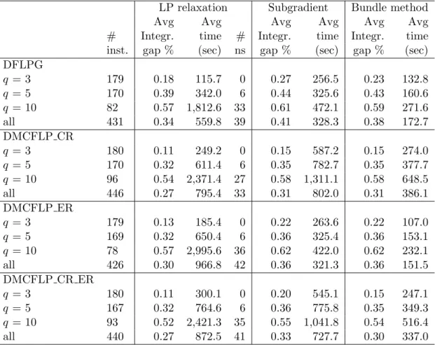
LP relaxation Subgradient Bundle method
Avg Avg Avg Avg Avg Avg
# Integr. time # Integr. time Integr. time
inst. gap % (sec) ns gap % (sec) gap % (sec)
DFLPG
q = 3 179 0.18 115.7 0 0.27 256.5 0.23 132.8
q = 5 170 0.39 342.0 6 0.44 325.6 0.43 160.6
q = 10 82 0.57 1,812.6 33 0.61 472.1 0.59 271.6
all 431 0.34 559.8 39 0.41 328.3 0.38 172.7
DMCFLP CR
q = 3 180 0.11 249.2 0 0.15 587.2 0.15 274.0
q = 5 170 0.32 611.4 6 0.35 782.7 0.35 377.7
q = 10 96 0.54 2,371.4 27 0.58 1,311.1 0.58 648.5
all 446 0.27 795.4 33 0.31 802.0 0.31 386.1
DMCFLP ER
q = 3 179 0.13 185.4 0 0.22 263.6 0.22 107.0
q = 5 169 0.32 650.4 6 0.36 325.4 0.36 153.1
q = 10 78 0.57 2,995.6 36 0.62 422.0 0.62 232.1
all 426 0.30 966.8 42 0.36 321.3 0.36 151.5
DMCFLP CR ER
q = 3 180 0.11 300.1 0 0.20 545.1 0.15 247.1
q = 5 167 0.32 764.6 6 0.36 775.8 0.35 349.3
q = 10 93 0.52 2,421.3 35 0.55 1,041.8 0.54 516.4
all 440 0.27 872.5 41 0.33 727.7 0.30 337.0
1 focuses on those instances and compares the average integrality gaps obtained when using the
bounds provided by the LP relaxation, as well as the two Lagrangian relaxation based methods. The subgradient and bundle methods have been stopped after a maximum of 1,000 and 500 iterations,
respectively. Column “# ns” indicates the number of instances for which the LP relaxation has
not been solved within 6 hours of computing time. This has typically been the case for larger problems, whereas the Lagrangian based methods provide bounds (and, of course, solutions) for
all instances. The average integrality gaps and average computing times have been computed over
the remaining instances that have been solved, and for which the optimal solution is known within 1%. For these instances (“# inst.”), the Lagrangian relaxation based methods are much faster.
Their integrality gaps are slightly higher, given that they perform a limited number of iterations.
In general, the GMC based models provide quite low integrality gaps. An analysis showed that the integrality gap has been found to be smaller than or equal to 1% for a fairly large part of the
instances. To be precise, the integrality gap is smaller than or equal to 1% for at least 413, 397, 410 and 397 instances for each of the four problems, respectively. The Lagrangian heuristics may
therefore prove optimality within a deviation of 1% for a large part of the instances, given that its
lower bounds are close to the LP relaxation bounds. Solving multi-period facility location problems within 1% of optimality is most likely sufficient for practical purposes (Melo et al., 2011), given
that the real data will slightly deviate from the forecast used to define the model.
5.2 Comparison of Different Configurations for the Lagrangian Heuristics
Section 3 discussed the subgradient method and the bundle method to solve the Lagrangian dual.
These methods can be used to generate feasible solutions at each iteration. Furthermore, informa-tion from the Lagrangian soluinforma-tions and the convexified bundle soluinforma-tions can be collected throughout
the solution of the Lagrangian dual (see Section 4), and then be used to generate a restricted MIP in
an attempt to find solutions of even better quality. We now compare the quality of those solutions.
Parameter Settings. The subgradient method is used with an initial scalar δ0 = 2.0. This
scale factor halves every 25 consecutive iterations without improvement in the lower bound. The
algorithm terminates ifδk falls below 0.005. For the bundle method, an implementation similar to the one described by Frangioni (2005) has been used as a black box. The bundle implementation has
four principal internal performance and termination criteria, which are set as follows. Parameters
5.2.1 Combining the Lagrangian Dual Solution Methods with a Restricted MIP
After performing the subgradient method, a restricted MIP can be solved based on the Lagrangian
solutions (see Section 4.1). When using the bundle method, the restricted MIP can further be generated on the convexified bundle solution (see Section 4.2). We now compare the performance
of different combinations for the heuristic, i.e., the use of the subgradient method and the bundle method to solve the Lagrangian dual, and the use of the restricted MIP based on Lagrangian
solutions and the convexified solutions to further improve the solution quality. Given the fast
convergence of the bundle method, we limit it to a maximum of 500 iterations. For the subgradient method, due to its slower convergence, we tested configurations with a maximum of 500 and 1,000
iterations.
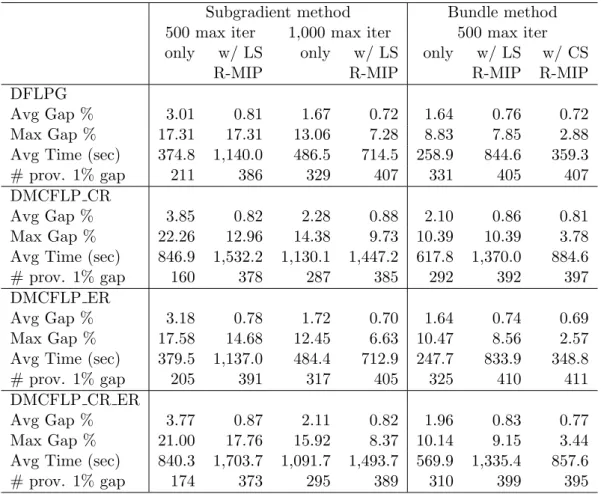
Table 2 summarizes the results for seven different solution strategies: the subgradient method without (“only”) and with a restricted MIP based on the Lagrangian Solutions (“w/ LS R-MIP”), as well as the bundle method without (“only”) and with a restricted MIP, based either on the Lagrangian solutions (“w/ LS R-MIP”) or on the convexified bundle solution (“w/ CS R-MIP”). When using the restricted MIP based on the Lagrangian solutions, we use parameter values that
have led to good performance (see Section 5.2.2): pF ix = 0.7 and nS = 3. For the aggregated bundle method with the restricted MIP based on the convexified solutions, we used pF ix= 0.85 and nS= 4, which led to smaller average and maximum optimality gaps than setting pF ix to 0.7, 0.8 or 0.9. Note that for the restricted MIP based on the convexified solutions, we only testednS
values of 2, 3 and 4.
The results take into account all 540 instances and are reported for each of the four problem
variants. We indicate the average and maximum gap (when compared to the best lower bounds
known for the instances), the average computing time and the number of instances for which a 1% optimality gap has been proved (“# prov. 1% gap”).
The results are consistent for the four different problem variants. Solving only the Lagrangian
dual, the bundle method clearly stays ahead of the subgradient method in terms of computing times. Due to its slower convergence, the subgradient method requires a maximum of 1,000 iterations to
reach a solution quality similar to that of the bundle method. After this first phase, a 1% optimality
gap has been proved for more than half of the instances.
Adding the Lagrangian solution based restricted MIP to the subgradient method significantly
improves the optimality gap when up to 1,000 iterations are performed. With only 500 iterations, the improvement is less significant. This illustrates the importance of reasonably solving the
La-grangian dual before constructing a restricted MIP, because “high-quality” decisions tend to appear
in the later stage of the subgradient method.
For the bundle method, a larger improvement of the maximum optimality gap can be observed.
The restricted MIP based on the convexified solution results in very competitive results. The
Subgradient method Bundle method
500 max iter 1,000 max iter 500 max iter
only w/ LS only w/ LS only w/ LS w/ CS
R-MIP R-MIP R-MIP R-MIP
DFLPG
Avg Gap % 3.01 0.81 1.67 0.72 1.64 0.76 0.72
Max Gap % 17.31 17.31 13.06 7.28 8.83 7.85 2.88
Avg Time (sec) 374.8 1,140.0 486.5 714.5 258.9 844.6 359.3
# prov. 1% gap 211 386 329 407 331 405 407
DMCFLP CR
Avg Gap % 3.85 0.82 2.28 0.88 2.10 0.86 0.81
Max Gap % 22.26 12.96 14.38 9.73 10.39 10.39 3.78
Avg Time (sec) 846.9 1,532.2 1,130.1 1,447.2 617.8 1,370.0 884.6
# prov. 1% gap 160 378 287 385 292 392 397
DMCFLP ER
Avg Gap % 3.18 0.78 1.72 0.70 1.64 0.74 0.69
Max Gap % 17.58 14.68 12.45 6.63 10.47 8.56 2.57
Avg Time (sec) 379.5 1,137.0 484.4 712.9 247.7 833.9 348.8
# prov. 1% gap 205 391 317 405 325 410 411
DMCFLP CR ER
Avg Gap % 3.77 0.87 2.11 0.82 1.96 0.83 0.77
Max Gap % 21.00 17.76 15.92 8.37 10.14 9.15 3.44
Avg Time (sec) 840.3 1,703.7 1,091.7 1,493.7 569.9 1,335.4 857.6
# prov. 1% gap 174 373 295 389 310 399 395
a 1% optimality gap could be proved increased to over 75% of all instances. While both approaches
show similar maximum optimality gaps, the convexified solution presents better average gaps and is capable of proving a 1% gap for more instances.
As previously mentioned, the use of a disaggregated bundle method did not lead to competitive
results for the problems discussed in this paper. For the DMCFLP CR ER with q = 10, the aggregated bundle method resulted in an average optimality gap of 4.05%, a maximum gap of
10.17% and converged, on average, after 424 iterations in 1,028.8 seconds. For the disaggregated method, different configurations of the bundle parameters have been tested. Allowing up to 25
subgradients for each block, the method resulted in an average optimality gap of 7.84%, a maximum
gap of 24.73% and converged, on average, after 429 iterations in 2,316.2 seconds. Allowing larger bundles improved the convergence (e.g., 198 iterations when up to 200 subgradients are used for
each block). However, computing times remained equally high, since the quadratic stabilization
involves the solution of a quadratic problem at each iteration, whose complexity increases as the bundle gets larger. Using linear instead of quadratic stabilization resulted in a faster solution of
the master problem, but deteriorated the convergence and therefore worsened computing times and
optimality gaps. Further, adding a restricted MIP model after the bundle method only marginally improved the solution quality, given that the solution of the Lagrangian dual consumes most of the
available time.
The results based on the aggregated bundle method are clearly better than those based on the subgradient method, as the subgradient method itself already takes a significant portion of the
available computing time. Therefore, there is often not enough time left to solve the restricted
MIP. However, a heuristic based on the latter could still be effective. Tuning the maximum number of subgradient iterations and the parameters used to define the restricted MIP will hereby make
the crucial difference. Such tuning is exemplified in the next section.
5.2.2 Restricted MIP Parameter Tuning
Given that the computing time limit includes the time to solve the restricted MIP after the solution
of the Lagrangian dual, this MIP has to be restricted sufficiently so that it can be reasonably solved
within the remaining time. This is done by appropriately setting the two parametersnS andpF ix, indicating the maximum number of decisions considered for each location and time period, and the
percentage necessary to fix a decision, respectively.
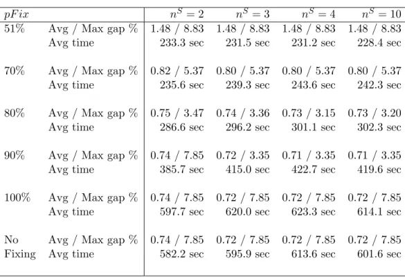
Table 3 summarizes the results for different parameter values, using the bundle method with a restricted MIP based on the convexified bundle solution applied to the DFLPG. The results
are given for all combinations between different pF ix and nS values, reporting the average and maximum optimality gap, as well as the average computation time. The average computation times increase due to two factors: more capacity level decisions in the MIP (i.e., higher values of
pF ix nS = 2 nS= 3 nS = 4 nS = 10
51% Avg / Max gap % 1.48 / 8.83 1.48 / 8.83 1.48 / 8.83 1.48 / 8.83
Avg time 233.3 sec 231.5 sec 231.2 sec 228.4 sec
70% Avg / Max gap % 0.82 / 5.37 0.80 / 5.37 0.80 / 5.37 0.80 / 5.37
Avg time 235.6 sec 239.3 sec 243.6 sec 242.3 sec
80% Avg / Max gap % 0.75 / 3.47 0.74 / 3.36 0.73 / 3.15 0.73 / 3.20
Avg time 286.6 sec 296.2 sec 301.1 sec 302.3 sec
90% Avg / Max gap % 0.74 / 7.85 0.72 / 3.35 0.71 / 3.35 0.71 / 3.35
Avg time 385.7 sec 415.0 sec 422.7 sec 419.6 sec
100% Avg / Max gap % 0.74 / 7.85 0.72 / 7.85 0.72 / 7.85 0.72 / 7.85
Avg time 597.7 sec 620.0 sec 623.3 sec 614.1 sec
No Avg / Max gap % 0.74 / 7.85 0.72 / 7.85 0.72 / 7.85 0.72 / 7.85
Fixing Avg time 582.2 sec 595.9 sec 613.6 sec 601.6 sec
Table 3: Comparison of results for different parameters for the bundle method with MIP based on the convexified bundle solution, applied to the DFLPG.
performing values can be found by balancing these two parameters. SettingnS to 3, 4 or even 10, andpF ixbetween 80% and 90% results in a maximum optimality gap of around 3.36%, while other parameter values may result in gaps of up to 8.83%. Clearly, if more computing time is available,
one may allow higher values for these parameters, which may further improve the solution quality.
Similar experiments were performed for different parameter values for the restricted MIP based on the Lagrangian solutions. It was found that the restricted MIP based on the Lagrangian solutions
is more sensitive to changes in the parameter value pF ix than the one based on the convexified bundle solution. This suggests that the decisions that are part of solutions selected by the bundle
are also present in high quality solutions.
5.3 Comparisons with CPLEX
The performance of one of the Lagrangian relaxation based heuristics is now compared to CPLEX.
We chose the configuration that provided the lowest average and maximum optimality gaps: the bundle method with restricted MIP based on its convexified solution, withnS = 4 andpF ix= 0.85.
but enable CPLEX to generate cover cuts that further strengthen the MIP formulation:
X
j∈J
X
`∈L
X
`0∈L−(j,t,`)
uj`0yjt``0 ≥
X
i∈I
X
p∈P
dtip ∀t∈T. (9)
As in the previous experiments, a 1% optimality stopping criterion and a time limit of 2 hours have been applied.
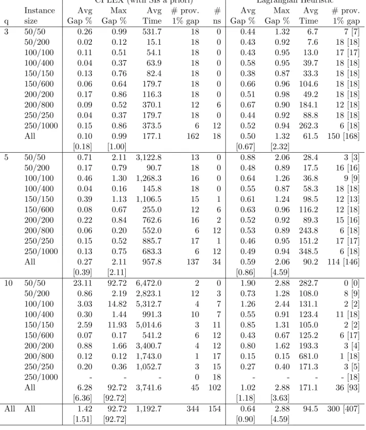
Tables 4 – 7 summarize the results for CPLEX, as well as for the Lagrangian based heuristic
outlined above for the four different problems DFLPG, DMCLFP CR, DMCFLP ER and DM-CFLP CR ER, respectively. All results are grouped by the number of capacity levels q and the
problem dimension defined by the number of candidate facility locations and the number of
cus-tomers. Each group given by such a combination includes 18 instances. The tables report the average and maximum gaps of the best feasible integer solutions found by the algorithm when
compared to the best lower bound known for the corresponding problem instance, as well as the
average computing times. Note that the results shown in the Tables 4 – 7 only take into account the instances where CPLEX found a feasible integer solution within the time limit of 2 hours. The
number of instances for which CPLEX did not find any feasible solution is indicated by column
“#ns”. Furthermore, column “# prov. 1% gap” gives the number of instances (out of those for which CPLEX found a feasible solution) where a 1% optimality gap has been proven by the
algo-rithm. For the Lagrangian heuristic, the number in brackets represents the same count, but for all instances, not only for those for which CPLEX found a feasible integer solution.
The observations made for the results of CPLEX and the Lagrangian based heuristics are similar
for all four problems. The number of instances where CPLEX did not find feasible solutions is fairly high, at least 25% of the instances for each of the four problems. In most of the cases, this happens
due to memory limitations when the number of capacity levels or the number of candidate facility
locations is high. Even though the average quality of solutions found by CPLEX is quite good, the solver provides large optimality gaps on many instances. This is mostly the case when a large
number of capacity levels (q = 10) is available. As the solver constantly improves its bounds,
the optimality gaps proven by the algorithm (shown in brackets) are very close to the gaps when compared to the best known lower bound for the instances. CPLEX is capable of proving a 1%
optimality gap for at least 342 out of the 540 instances for each of the four problems.
The Lagrangian based heuristic provides stable results for each of the four problems. When compared to the same instances, it provides an average gap lower than that of CPLEX in
com-puting times that are, on average, significantly lower. For the DFLPG and the DMCFLP ER,
the Lagrangian heuristic is, on average, twelve times faster than CPLEX. For the DMCFLP CR and the DMCFLP CR ER, the heuristic is, on average, five times faster. Most importantly, the
maximum optimality gap is at most 3.78%. Due to the strength of the GMC formulation, the
CPLEX. When considering all 540 instances (even those for which CPLEX does not find feasible
solutions), the Lagrangian heuristic proves a 1% gap for 395 or more of the 540 instances for each of the four problems.
Interestingly, the difficulty of a problem is not always linked to its dimension. Instances where
the number of customers is close to the number of candidate facility locations are significantly harder to solve than those where the number of customers is higher. In particular, this can be observed
for instances of dimension (50/50). An analysis showed that these instances tend to possess larger integrality gaps, which may be linked to the fact that the more customers are available, the easier
it is to make efficient use of a facility (in terms of allocation costs and capacity usage) in an integer
solution.
To assess the capability of CPLEX to tackle the problems when a larger time limit is given,
additional experiments with a time limit of 24 hours have been performed for the four problem
variants. The results only slightly improved when compared to the results with a time limit of two hours. For the 180 instances with q = 10, the average optimality gaps have been found to
be 1.95%, 1.55%, 0.90% and 2.40% for the DFLPG, the DMCFLP CR, the DMCFLP ER and the
DMCFLP CR ER, respectively. CPLEX did not find any feasible solution for 85, 69, 76 and 79 instances, respectively, mostly due to the high memory consumption when solving the LP relaxation.
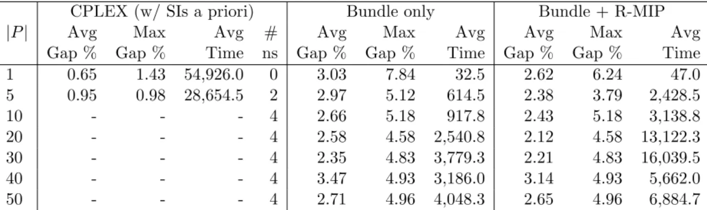
Impact of the Number of Commodities. The instances used in the previous experiments
contain up to five different commodities. We now explore the scalability of the methods in terms of the number of commodities. Problem instances of sizes (50/50) and (50/200) have been generated
with 1, 2, 5, 10, 20, 30, 40 and 50 different commodities in the same manner as the previous problem
instances. The demand has then been scaled by multiplying by |P2| to avoid a total demand that is too high (which may result in an optimal solution that opens all facilities). Table 8 summarizes the
results for CPLEX and for two variants of the Lagrangian heuristic based on the aggregated bundle method, each approach limited to a total of 24 hours of computing time. Each line considers four
instances with a different number of commodities |P|. The reported average and maximum gaps
are those proven by the algorithms, since the instances were too large to be solved exactly. Using CPLEX, the models exceed the memory limit of 24GB when the problem contains five commodities
or more, as can be seen in the column that indicates the number of instances for which no feasible
solution has been found (’# ns’). In contrast, the Lagrangian heuristics find solutions and prove reasonably low optimality gaps for all instances. The heuristic using only the bundle method proves
a maximum gap of 7.84%. The computing times for the bundle method are quite predictable, as the
number of commodities only impacts the solution time of the transportation problems that have to be solved in the Lagrangian subproblems. The average computing times remain, on average, below
two hours. The improvement of the optimality gaps when adding the restricted MIP (with identical
CPLEX (with SIs a priori) Lagrangian Heuristic
Instance Avg Max Avg # prov. # Avg Max Avg # prov.
q size Gap % Gap % Time 1% gap ns Gap % Gap % Time 1% gap
3 50/50 0.26 0.99 531.7 18 0 0.44 1.32 6.7 7 [7]
50/200 0.02 0.12 15.1 18 0 0.43 0.92 7.6 18 [18]
100/100 0.11 0.51 54.1 18 0 0.43 0.95 13.0 17 [17]
100/400 0.04 0.37 63.9 18 0 0.58 0.95 39.7 18 [18]
150/150 0.13 0.76 82.4 18 0 0.38 0.87 33.3 18 [18]
150/600 0.06 0.64 179.7 18 0 0.66 0.96 104.6 18 [18]
200/200 0.17 0.86 116.3 18 0 0.51 0.98 49.2 18 [18]
200/800 0.09 0.52 370.1 12 6 0.67 0.90 184.1 12 [18]
250/250 0.04 0.37 179.7 18 0 0.44 0.92 88.8 18 [18]
250/1000 0.15 0.86 373.5 6 12 0.52 0.94 262.3 6 [18]
All 0.10 0.99 177.1 162 18 0.50 1.32 61.5 150 [168]
[0.18] [1.00] [0.67] [2.32]
5 50/50 0.71 2.11 3,122.8 13 0 0.88 2.06 28.4 3 [3]
50/200 0.17 0.79 90.7 18 0 0.48 0.89 17.5 16 [16]
100/100 0.46 1.30 1,268.3 16 0 0.64 1.26 36.8 9 [9]
100/400 0.04 0.16 145.8 18 0 0.55 0.87 58.3 18 [18]
150/150 0.39 1.13 1,106.5 15 1 0.61 1.24 98.5 12 [13]
150/600 0.08 0.67 255.0 12 6 0.63 0.96 116.2 12 [18]
200/200 0.22 0.84 762.6 16 2 0.52 0.92 89.3 15 [16]
200/800 0.06 0.20 552.0 6 12 0.53 0.89 243.8 6 [18]
250/250 0.15 0.52 885.7 17 1 0.46 0.95 151.2 17 [17]
250/1000 0.13 0.75 683.3 6 12 0.49 0.94 348.5 6 [18]
All 0.27 2.11 957.8 137 34 0.59 2.06 90.2 114 [146]
[0.39] [2.11] [0.86] [4.59]
10 50/50 23.11 92.72 6,472.0 2 0 1.90 2.88 282.7 0 [0]
50/200 0.86 2.19 2,823.1 12 3 0.73 1.28 108.0 8 [9]
100/100 3.03 14.82 5,312.7 4 7 1.26 2.44 131.1 2 [2]
100/400 0.30 1.44 991.3 10 7 0.55 0.91 123.4 11 [18]
150/150 2.59 11.93 5,014.6 3 11 0.85 1.31 105.0 2 [2]
150/600 0.07 0.17 541.2 6 12 0.43 0.67 125.2 6 [17]
200/200 0.88 1.66 3,400.7 4 12 0.80 1.62 193.3 3 [4]
200/800 0.12 0.12 1,743.0 1 17 0.15 0.15 681.0 1 [18]
250/250 0.20 0.36 1,052.7 3 15 0.27 0.40 171.3 3 [5]
250/1000 - - - 0 18 - - - - [18]
All 6.28 92.72 3,741.6 45 102 1.02 2.88 171.1 36 [93]
[6.36] [92.72] [1.18] [3.63]
All All 1.42 92.72 1,192.7 344 154 0.64 2.88 94.5 300 [407]
[1.51] [92.72] [0.90] [4.59]
CPLEX (with SIs a priori) Lagrangian Heuristic
Instance Avg Max Avg # prov. # Avg Max Avg # prov.
q size Gap % Gap % Time 1% gap ns Gap % Gap % Time 1% gap
3 50/50 0.29 1.14 650.6 17 0 0.51 1.54 13.9 7 [7]
50/200 0.08 0.67 18.5 18 0 0.61 0.99 15.6 18 [18]
100/100 0.11 0.55 41.2 18 0 0.44 0.84 27.3 17 [17]
100/400 0.08 0.66 90.6 18 0 0.62 0.94 86.8 18 [18]
150/150 0.04 0.23 102.4 18 0 0.52 0.99 62.4 18 [18]
150/600 0.10 0.85 275.5 18 0 0.72 0.98 243.4 18 [18]
200/200 0.13 0.92 198.0 18 0 0.56 0.95 137.8 16 [16]
200/800 0.19 0.93 589.3 12 6 0.57 0.95 530.9 12 [18]
250/250 0.06 0.34 496.3 18 0 0.56 0.95 219.1 18 [18]
250/1000 0.15 0.73 791.0 6 12 0.67 0.96 596.7 6 [18]
All 0.12 1.14 281.1 161 18 0.57 1.54 151.0 148 [166]
[0.19] [1.27] [0.74] [2.75]
5 50/50 0.67 2.44 1,973.7 14 0 0.91 2.24 32.2 3 [3]
50/200 0.26 0.69 86.4 18 0 0.54 1.04 46.9 16 [16]
100/100 0.37 0.93 1,144.2 17 0 0.45 1.05 91.8 13 [13]
100/400 0.11 0.89 203.6 18 0 0.61 0.97 136.9 18 [18]
150/150 0.39 1.00 1,104.5 17 0 0.54 1.19 191.7 15 [15]
150/600 0.09 0.85 413.8 12 6 0.69 0.95 280.6 12 [18]
200/200 0.23 0.88 992.8 18 0 0.52 0.96 322.6 18 [18]
200/800 0.16 0.60 868.0 6 12 0.36 0.94 597.0 6 [18]
250/250 0.48 3.88 1,473.8 16 1 0.54 1.12 457.3 16 [17]
250/1000 0.16 0.81 1,214.5 6 12 0.64 0.98 734.3 6 [18]
All 0.32 3.88 950.4 142 31 0.59 2.24 227.7 123 [154]
[0.47] [3.95] [0.89] [3.70]
10 50/50 4.27 19.79 5,779.7 4.00 1 2.32 3.78 977.8 0 [0]
50/200 0.74 1.51 3,308.0 9 5 0.82 1.53 202.8 4 [4]
100/100 7.84 66.50 5,449.2 4 5 1.67 3.19 376.4 0 [0]
100/400 0.92 8.29 1,151.1 11 6 0.66 0.99 370.7 11 [15]
150/150 17.03 88.13 5,172.8 4 7 1.26 2.40 331.3 1 [1]
150/600 0.26 0.89 1,010.3 6 12 0.55 0.88 440.5 6 [15]
200/200 23.45 89.67 4,217.1 4 10 1.09 1.73 506.6 3 [3]
200/800 0.22 0.63 3,467.8 6 12 0.44 0.95 1,395.0 6 [17]
250/250 1.02 2.91 3,064.0 3 14 0.52 0.80 664.8 4 [6]
250/1000 - - - 0 18 - - - - [16]
All 6.41 89.67 3,951.9 51 90 1.23 3.78 555.2 35 [77]
[7.08] [100.00] [1.53] [4.50]
All All 1.61 89.67 1,353.7 354 139 0.72 3.78 270.2 306 [397]
[1.84] [100.00] [1.05] [4.50]
CPLEX (with SIs a priori) Lagrangian Heuristic
Instance Avg Max Avg # prov. # Avg Max Avg # prov.
q size Gap % Gap % Time 1% gap ns Gap % Gap % Time 1% gap
3 50/50 0.25 0.94 779.8 17 0 0.25 0.86 6.7 11 [11]
50/200 0.01 0.10 20.5 18 0 0.59 0.97 6.9 18 [18]
100/100 0.17 0.67 40.7 18 0 0.37 0.94 13.8 17 [17]
100/400 0.04 0.37 89.0 18 0 0.65 0.99 40.7 18 [18]
150/150 0.20 0.74 120.3 18 0 0.46 0.96 26.4 18 [18]
150/600 0.01 0.17 263.9 18 0 0.67 0.95 105.0 18 [18]
200/200 0.06 0.43 189.7 18 0 0.31 0.86 46.3 18 [18]
200/800 0.11 0.76 466.3 12 6 0.75 0.96 190.3 12 [18]
250/250 0.04 0.40 393.0 18 0 0.50 0.91 97.1 18 [18]
250/1000 0.31 0.91 538.8 6 12 0.50 0.91 247.3 6 [18]
All 0.11 0.94 265.3 161 18 0.50 0.99 61.4 154 [172]
[0.20] [1.39] [0.68] [2.11]
5 50/50 0.56 1.60 2,521.3 15 0 0.85 1.79 34.7 3 [3]
50/200 0.19 0.65 100.7 18 0 0.48 0.86 18.3 15 [15]
100/100 0.44 1.83 1,376.8 15 0 0.58 1.35 35.1 10 [10]
100/400 0.10 0.45 240.1 18 0 0.57 0.83 58.2 18 [18]
150/150 0.43 1.44 1,286.9 16 0 0.50 1.21 91.9 13 [13]
150/600 0.01 0.11 393.4 12 6 0.67 0.97 118.4 12 [18]
200/200 0.38 2.58 1,061.8 16 1 0.53 0.98 113.6 16 [16]
200/800 0.05 0.11 796.5 6 12 0.51 0.94 239.0 6 [18]
250/250 0.17 0.63 1,211.4 16 2 0.51 0.91 174.9 16 [17]
250/1000 0.32 0.82 1,076.8 6 12 0.54 0.94 328.2 6 [18]
All 0.29 2.58 1,039.8 138 33 0.58 1.79 94.2 115 [146]
[0.43] [2.60] [0.87] [3.84]
10 50/50 6.31 87.99 5,595.0 6.00 0 1.44 2.57 149.9 1 [1]
50/200 0.83 5.76 2,029.6 15 1 0.64 1.19 125.5 9 [10]
100/100 8.18 91.36 4,867.1 6 3 1.22 2.43 157.3 2 [2]
100/400 0.23 0.63 1,012.0 11 7 0.51 0.86 125.1 11 [17]
150/150 11.78 95.92 5,188.2 4 9 1.06 1.92 570.4 2 [2]
150/600 0.09 0.31 1,139.2 6 12 0.44 0.67 154.3 6 [16]
200/200 0.61 1.91 2,713.2 4 13 0.80 1.48 166.0 2 [3]
200/800 3.20 6.33 3,544.0 1 16 0.02 0.04 507.0 2 [18]
250/250 0.10 0.19 1,570.0 3 15 0.40 0.84 165.3 3 [6]
250/1000 - - - 0 18 - - - - [18]
All 4.30 95.92 3,468.0 56 94 0.91 2.57 197.3 38 [93]
[4.62] [100.00] [1.18] [3.83]
All All 1.09 95.92 1,250.8 355 145 0.62 2.57 103.2 307 [411]
[1.25] [100.00] [0.91] [3.84]
CPLEX (with SIs a priori) Lagrangian Heuristic
Instance Avg Max Avg # prov. # Avg Max Avg # prov.
q size Gap % Gap % Time 1% gap ns Gap % Gap % Time 1% gap
3 50/50 0.23 1.20 738.9 17 0 0.48 1.40 13.9 7 [7]
50/200 0.05 0.44 20.6 18 0 0.46 0.94 16.0 18 [18]
100/100 0.15 0.73 70.4 18 0 0.38 0.93 32.5 17 [17]
100/400 0.13 0.87 99.0 18 0 0.53 0.90 84.5 18 [18]
150/150 0.09 0.39 127.3 18 0 0.49 0.94 58.3 18 [18]
150/600 0.03 0.28 302.9 18 0 0.74 0.97 217.0 18 [18]
200/200 0.13 0.79 248.5 18 0 0.52 0.96 126.4 18 [18]
200/800 0.15 0.93 666.7 12 6 0.64 0.98 422.9 12 [18]
250/250 0.11 0.83 453.1 18 0 0.41 0.87 201.0 18 [18]
250/1000 0.04 0.12 812.3 6 12 0.69 0.95 428.2 6 [18]
All 0.12 1.20 308.4 161 18 0.52 1.40 130.5 150 [168]
[0.19] [1.23] [0.68] [2.39]
5 50/50 0.71 2.96 2,951.6 13 0 0.91 2.42 48.4 3 [3]
50/200 0.23 0.81 187.3 18 0 0.45 0.82 41.4 14 [14]
100/100 0.47 1.85 1,286.9 16 0 0.54 1.42 88.8 10 [10]
100/400 0.12 0.63 273.7 18 0 0.55 0.95 129.6 18 [18]
150/150 0.41 1.13 1,242.1 16 1 0.52 0.87 164.8 15 [15]
150/600 0.10 0.89 475.3 12 6 0.67 0.96 242.3 12 [18]
200/200 0.26 0.84 1,193.9 18 0 0.40 0.86 319.4 17 [17]
200/800 0.17 0.89 1,202.3 6 12 0.68 0.97 599.5 6 [18]
250/250 0.47 4.61 1,230.1 15 2 0.52 0.98 358.8 16 [17]
250/1000 0.03 0.15 1,347.3 6 12 0.66 0.86 640.3 6 [18]
All 0.33 4.61 1,142.0 138 33 0.57 2.42 205.3 117 [148]
[0.47] [4.61] [0.87] [4.00]
10 50/50 8.06 87.78 6,168.2 3.00 0 2.14 3.44 1,632.8 0 [0]
50/200 0.63 1.55 2,561.8 11 5 0.70 1.23 172.5 6 [7]
100/100 15.65 94.16 5,781.8 3 4 1.72 2.59 776.1 0 [0]
100/400 0.28 0.68 705.1 10 8 0.66 0.96 194.3 10 [14]
150/150 0.98 1.82 4,655.6 4 11 1.02 1.66 289.4 1 [1]
150/600 0.04 0.19 1,394.0 6 12 0.53 0.99 492.5 6 [15]
200/200 19.75 96.06 4,567.4 3 13 0.97 1.69 384.0 2 [2]
200/800 - - - 0 18 - - - - [17]
250/250 0.23 0.50 3,733.7 3 15 0.40 0.57 453.3 3 [6]
250/1000 - - - 0 18 - - - - [17]
All 6.34 96.06 4,043.6 43 104 1.24 3.44 693.4 28 [79]
[6.74] [100.00] [1.44] [4.87]
All All 1.43 96.06 1,364.1 342 155 0.68 3.44 270.2 295 [395]
[1.59] [100.00] [1.00] [4.87]
CPLEX (w/ SIs a priori) Bundle only Bundle + R-MIP
|P| Avg Max Avg # Avg Max Avg Avg Max Avg
Gap % Gap % Time ns Gap % Gap % Time Gap % Gap % Time
1 0.65 1.43 54,926.0 0 3.03 7.84 32.5 2.62 6.24 47.0
5 0.95 0.98 28,654.5 2 2.97 5.12 614.5 2.38 3.79 2,428.5
10 - - - 4 2.66 5.18 917.8 2.43 5.18 3,138.8
20 - - - 4 2.58 4.58 2,540.8 2.12 4.58 13,122.3
30 - - - 4 2.35 4.83 3,779.3 2.21 4.83 16,039.5
40 - - - 4 3.47 4.93 3,186.0 3.14 4.93 5,662.0
50 - - - 4 2.71 4.96 4,048.3 2.65 4.96 6,884.7
Table 8: Comparison of CPLEX and Lagrangian based heuristics for problem instances of with 50 facility locations and different numbers of commodities for the DMCFLP CR ER: average and maximum of the proven optimality gaps.
A Note on the Model Size. As the previous results show, general-purpose MIP solvers such as CPLEX may perform very well on small instances, i.e., when the number of capacity levels is low
(q ∈ {3,5}) and the number of candidate facility locations is small (|J| ≤100). Clearly, adding the
SIs (4) a priori to the model significantly increases the number of constraints and, therefore, the memory requirements of the model. As noted by Jena et al. (2015a), the addition of the SIs to the
GMC based models significantly facilitates the solution of the problems. In fact, for the instances used in this work, without the use of the SIs, CPLEX provides very low quality solutions even
for small instances. While certain studies (e.g., Gendron and Larose, 2014, for a network design
problem) indicate that it may be beneficial to add these inequalities in a branch-and-cut scheme, this only yields good performance if a small number of SIs are violated and therefore added to the
model. In the case of the DFLPG, the number of violated SIs is rather high and adding them as
user cuts provided less competitive results. For more than 40% of the instances, the solver could not find feasible solutions. When feasible solutions were found, the average optimality gap was
consistently high, on average, more than 10%.
We also note that, even though we use information from the Lagrangian solutions, other mech-anisms could be used to rate the importance of opening decisions to generate a MIP that is
signifi-cantly restricted in size. Theoretically, using the LP relaxation solution is an alternative. However,
as the LP relaxation cannot be efficiently solved (or not at all) for large instances, such a so-lution strategy would be applicable only to small and medium sized instances, or in computing
environments with significantly larger memory and time resources.
6
Conclusions
In this work, we have extended the Dynamic Facility Location Problem with Generalized Modular
Capacities by considering demands for multiple commodities. We addressed the solution of
dual is solved, involving the iterated solution of the Lagrangian subproblem. In this phase, feasible
solutions of reasonable quality are found in very short computing times. Then, a restricted MIP is generated taking into consideration only decisions that have been found to be important during
the solution of the Lagrangian dual. Using this approach, the final solution quality is consistently
within 3.78% from the best known lower bound, even for instances for which CPLEX does not find feasible solutions due to the large memory and solution time required by the model.
The general cost structure of this problem allows for representing several existing facility location
problems. In addition to the DFLPG, in which the capacity change costs are based on a cost matrix, this has been exemplified on three special cases. Given the strength of the GMC formulation, the
Lagrangian heuristic was able to prove optimality within 1% for most of the small and medium sized
instances. The proposed model and solution method may be applied to other problems, especially to those where the model size exceeds the limits of state-of-the-art MIP solvers. It may also be
applied to larger instances than those addressed in this work, as the method consumes very little memory.
The Lagrangian dual has been solved by the classical subgradient method and an aggregated
bundle implementation. Although the bundle method requires more time to compute the La-grangian multipliers, it consistently outperformed the subgradient approach due to its strong
con-vergence properties. On average, it required half of the time and resulted in a higher solution
quality.
While local improvement heuristics have been commonly used as a second phase optimization,
the use of a restricted MIP is an interesting alternative, as general-purpose MIP solvers constantly
improve. The implementation of a restricted MIP is very simple. Furthermore, one can handle any kind of problem structure that can be defined as a MIP. Even though one does not have to
worry about finding the right trade-off between size and inspection time of a neighborhood, the
question of how to significantly restrict the size of the original MIP is crucial. The bundle method with restricted MIP provided very competitive results, especially since the use of the convexified
solutions already limits the decisions to those stored in the bundle.
Acknowledgements
The authors are grateful to MITACS, the Natural Sciences and Engineering Research Council of Canada (NSERC) and the Fonds de recherche du Qu´ebec Nature et Technologies (FRQNT) for
their financial support. The authors would also like to thank Antonio Frangioni and Enrico Gorgone