Design and performance of a high-resolution frictional force microscope with
quantitative three-dimensional force sensitivity
M. Dienwiebel, E. de Kuyper, L. Crama, J. W. M. Frenken, J. A. Heimberg, D.-J. Spaanderman, D. Glastra van Loon, T. Zijlstra, and E. van der Drift
Citation: Review of Scientific Instruments 76, 043704 (2005); doi: 10.1063/1.1889233
View online: http://dx.doi.org/10.1063/1.1889233
View Table of Contents: http://aip.scitation.org/toc/rsi/76/4
Design and performance of a high-resolution frictional force microscope
with quantitative three-dimensional force sensitivity
M. Dienwiebel,a兲 E. de Kuyper, L. Crama, and J. W. M. Frenkenb兲
Kamerlingh Onnes Laboratory, Leiden University, P.O. Box 9506, 2300 RA Leiden, The Netherlands
J. A. Heimberg,c兲 D.-J. Spaanderman, and D. Glastra van Loon
FOM-Institute for Atomic and Molecular Physics, Kruislaan 407, 1098 SJ Amsterdam, The Netherlands
T. Zijlstra and E. van der Drift
Delft Institute of Microelectronics and Submicron Technology (DIMES), Delft University of Technology, P.O. Box 5053, 2600 GB Delft, The Netherlands
共Received 17 March 2004; accepted 22 January 2005; published online 1 April 2005兲
In this article, the construction and initial tests of a frictional force microscope are described. The instrument makes use of a microfabricated cantilever that allows one to independently measure the lateral forces in X and Y directions as well as the normal force. We use four fiber-optic interferometers to detect the motion of the sensor in three dimensions. The properties of our cantilevers allow easy and accurate normal and lateral force calibration, making it possible to measure the lateral force on a fully quantitative basis. First experiments on highly oriented pyrolytic graphite demonstrate that the microscope is capable of measuring lateral forces with a resolution down to 15 pN. © 2005 American Institute of Physics. 关DOI: 10.1063/1.1889233兴
I. INTRODUCTION
One of the oldest unresolved problems in physics con-cerns mechanisms of friction. This may seem surprising in the light of the fact that systematic research dates back to Leonardo da Vinci.1There is an impressive body of phenom-enological knowledge on friction, but most of this knowl-edge lacks a true understanding on a microscopic level. Questions about atomic-scale details of energy dissipation are becoming increasingly important as, e.g., technologies of data storage, microelectromechanical systems共MEMS兲 and specialized coatings advance. In these areas, the phenomeno-logical and often used friction law of Amontons and Cou-lomb, that the frictional force is linearly proportional to the normal force, does not always apply.2,3 In order to better predict and control tribological behavior on the small length scales involved, a truly microscopic understanding of friction and wear is required. Real surfaces in contact only truly meet at those points with the highest topography due to surface roughness共i.e., asperities兲. It has been shown that it is the statistics of these asperities that leads to the Amontons and Coulomb law.4As asperities move with respect to each other, the contributions of individual asperities to the friction force are averaged. One approach to obtain information on the tribological behavior of single asperities is to control the surfaces such that only one asperity is created. This area of research has come to be called nanotribology. It has long been recognized that the tip-on-flat geometry of an atomic
force microscope 共AFM兲 closely resembles a realistic asperity.5AFMs have been adapted to measure lateral forces down to the nanometer and nanonewton regimes by measur-ing the torsional response of the force probe. In the past, frictional force microscopes共FFMs兲have produced predomi-nantly qualitative results although recently some groups have succeeded in obtaining quantitative nanotribology results.3,6 Even as the techniques in traditional FFM become more re-fined, the basic problem remains that this method uses a force probe designed to be most sensitive to forces normal to the contact. The ramification of this is that most cantilevers snap into contact as the tip-to-sample distance approaches the near contact regime, so that the lateral forces are mea-sured in “hard” contact. This near-contact regime is of great technological importance as fly heights in disk drives de-crease and as the length scales in MEMS are reduced. Can-tilevers that do not suffer from the “snap-to-contact” problem will have large torsional spring constants so that small lateral forces cannot be detected. In most FFMs, only one compo-nent of the lateral force is measured. In addition, bending motion of standard cantilevers cannot be distinguished from buckling7 and it is very difficult to minimize coupling be-tween the normal and the torsional bending,8 which can be seen by the fact that the feedback parameters can have dra-matic influence on the measured friction signal.9This is also a fact well known and of equal frustration to the AFM com-munity. Our main objective was to build a quantitative FFM that would measure both lateral forces with better sensitivity and at smaller tip-sample separation distances than current FFMs. Ultimately it is our aim to atomically control the con-tact area between the tip and sample in UHV via field ion microscopy and field evaporation.10 Consideration of these requirements and future additions played an important role in
a兲Present address: IAVF Antriebstechnick AG, Im Schlehert 32, 76187
Karlsruhe, Germany.
b兲Electronic mail: [email protected]
c兲Present address: John Hopkins Applied Physics Laboratory, 11100 John
Hopkins Rd., Laurel, Maryland 20723-6099.
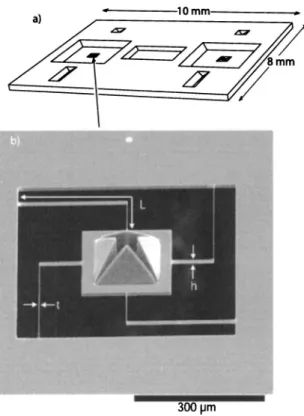
some of the design decisions for our prototype, ambient-condition FFM with three-dimensional detection. The instru-ment consists of two stages: the fiber head assembly contain-ing the detection system and the specialized lateral force cantilever, and the sample stage that allows for manipulation of the sample with respect to the tip and cantilever. We began our FFM design by first designing a dedicated force probe. The precise design and manufacturing details of this so-called “Tribolever®” have been reported in another article.11 A scanning electron microscope共SEM兲image of the monoc-rystalline monolithic silicon structure is seen in Fig. 1. Four high aspect ratio legs extend out from a central detection pyramid. A fiber optic interferometer reflects off of each pyramid face to track the motion of the pyramid. The scan-ning tip, which can be an etched metal wire, for example, tungsten, is threaded through the central hole of the pyramid and extends⬃50– 100m out from the base of the pyramid to interact with the surface. The shape and dimensions of the four legs have been chosen and tested using finite element analysis,12so that the two lateral spring constants are equal and significantly lower than the torsional spring constant of single board-type cantilevers used in AFMs. Using cantilever dimensions obtained from the literature,13 a typical torsional spring constant is 72 N / m, whereas the Tribolevers® lateral spring constants are typically kxTribolever⬅kyTribolever= 1.4 N / m. In the normal direction, kzAFM= 0.2 N / m, while kzTribolever = 10.6 N / m 共see below兲. Additionally, the coupling in the Tribolever between the three orthogonal directions is⬃10−6 and coupling between torsional共out of scanning plane兲and normal forces is essentially zero. The focus of the present article is on the apparatus, which houses, moves and
manipu-lates the optical fibers with respect to the detection pyramid and the tip-fiber head with respect to the sample. Initial re-sults are reported, and used to demonstrate the performance of this microscope.
II. INSTRUMENTATION
A. Detection principle
As discussed briefly above, the pyramid is in the center of the detection system, which consists of four all-fiber in-terferometers. Each of the four glass fibers is coupled to a laser diode and a photodiode detector as described in Sec. II B. The light that leaves the fiber at the end face is centered on one of the four pyramid faces. Part of that light is re-flected back into the fiber, where it interferes with the light that is reflected internally at the fiber end face. The interfer-ometer’s output is given by
I = I0
冋
1 + V cos冉
22D
冊
册
, 共1兲where I is the output current, V is the relative interference amplitude, D is the fiber-sample distance, andis the wave-length of the laser共780 nm in our case兲. The offset I0and the
amplitude V are both determined by the reflectivities of the two interfaces responsible for the interference signal. Spe-cifically, for the fiber/air interface a maximum reflectance of 4% is expected and for the pyramid surface a maximum re-flectance in the order of 60%. The pyramid, which is ap-proximately 80m high, with a 150-m-wide base, is formed via a KOH wet etch, which exposes the共111兲planes of silicon, which provides an area available for the fibers to reflect from of at least 1500m2. A special passivation tech-nique, necessary to protect the corners of the convex struc-ture from underetching,11 gives rise to the presence of a cross-shaped hole within the pyramid共Fig. 1兲. One advan-tage of this design is that the entire cantilever structure can be made out a single-crystal silicon wafer. The faces of the pyramid are highly reflective and of a well-defined angle, = 54.74°, with respect to the共100兲surface plane of the wafer. If each of the four glass fibers is adjusted such that the light intensity increases when the fiber-pyramid distance decreases
关Eq.共1兲兴the three-dimensional displacement with respect to the fixed fibers can be extracted from the normalized sum and differences of the signals coming from the four interferometers.14 These linear combinations need to be weighted by the appropriate geometrical projection共Fig. 2兲
X =X2− X1
2 sin, 共2兲
Y =Y2− Y1
2 sin, 共3兲
Z =X1+ X2+ Y1+ Y2
4 cos . 共4兲
B. Interferometers
The design of our interferometers follows closely those discussed in the literature,15,16 with attention given to the FIG. 1. Schematic of the “Tribolever®” device共a兲. The prototype chip
共10 mm⫻8 mm兲includes two force sensors, each with its own set of kine-matic mounts. SEM micrograph共b兲of the sensor. The dimensions of the legs of the sensor are L = 350m, t = 1.4m and h = 10.6m.
stability of the laser diode’s output intensity and wavelength.17 One unique aspect of our design is that each opposing pair of interferometers is driven by a single laser diode so that the influence of fluctuations in laser intensity and wavelength is greatly reduced, while the remaining variations can be divided out by use of a reference signal. A schematic of one such pair共e.g., the X pair兲is seen in Fig. 3. Light coming from the laser diode is first divided over two branches using a bidirectional 2⫻2 fiber coupler. The two branches are denoted with X1 and X2, respectively. A second 2⫻2 coupler in each arm completes the interferom-eter, by coupling out the backwards traveling reflected light into the photodiode detector. The same coupler couples out
50% of the the primary light into the reference signal detec-tor.
We see no evidence for optical coupling between the two fiber pairs. Such coupling was not expected, as little diffuse reflection occurs at the pyramid faces. As a result, we see no change in one pair, even when the other pair is optically disconnected. In order for the 125-m-diam fibers to be po-sitioned close the pyramid faces, they must be tapered to a maximum end face diameter of 80m.18We have used both sharpened fibers with cleaved end faces19 and fibers chemi-cally etched using the liquid layer protection procedure.20 The latter method results in fiber tips with a cone angle that can be varied from 8° to 41° depending on the protection fluid.21To create an end face the fiber tips were mechanically polished. The former method results in slightly stronger in-terference signals共presumably due to the cleave兲. The latter method routinely produces end face diameters on the order of 30m, which allows for more flexibility when position-ing all four fibers.
C. Fiberhead
To position the four fibers with respect to the silicon pyramid we constructed a special fiberhead共see Fig. 4兲. The fiberhead was machined by spark erosion from a single block of low-thermal-expansion metal共Invar兲. The distance of the end face of each fiber with respect to the pyramid face is adjusted by miniature inertial piezomotors共Nanomotors®22兲, that can either be driven in discrete steps over a maximum distance of approximately 4 mm or be adjusted continuously with sub-Å resolution over a range of 400 nm. The first mode allows one to retract the glass fibers to a safe distance during change of sensors, the latter is used to calibrate the interferometer signals and to position the fibers at the dis-tance of maximum sensitivity. Additionally the continuous FIG. 2. Schematic showing two of the four glass fibers. If the pyramid
moves laterally共a兲, the distance X1 between the left glass fiber and the pyramid increases and the distance X2 between the right glass fiber and the pyramid decreases or vice versa. If the pyramid moves normal to the sample surface, both distances either decrease or increase. This allows one to extract the displacements of the pyramid in the X and Z directions. Similarly, from the other fiber pair one obtains the displacements in the Y and Z directions. The displacements are extracted from the distance changes, according to Eqs.共2兲–共4兲.
FIG. 3. Components of one interferometer pair. The interferometer can be divided into three distinct sections: the laser system, the fiber system and the detection system. The laser system consists of the laser diode with integrated Faraday isolator and the controlling power supplies. The fiber system con-sists of couplers, connectors, adapters and the fiber itself. The detection system consists of photodiodes and supporting electronics.
mode can be used to compensate possible drift between the fibers and the pyramid due to thermal expansion of the mi-croscope 共see electronics section兲. The Nanomotors® are mounted in miniature flexure hinge springs, which are part of the fiber head. These springs allow the adjustment of each fiber axis in a plane parallel to the pyramid plane.
Different types of the Tribolever® can be clamped onto an exchangeable plate by means of two stiff leaf springs. On the backside of the cantilever plate, three small diameter ruby spheres are cemented. A quadrahedral hole-groove-flat-type kinematic mount is integrated into the silicon chip that houses the Tribolever®.23 The ruby spheres rest within the kinematic mount on each silicon chip. We have found that this system of kinematic mounts works so well that only little repositioning 共⬍10m兲 of the fibers via the flexure hinge springs is necessary between different cantilevers to restore optimal signals.
The fiberhead is fixed into an invar plate that matches the dimensions of the sample stage underneath. The com-plete assembly of the microscope can be seen in Fig. 5. The sample共restricted to lateral dimensions of 10⫻10 mm2兲sits on a scan tube,24 which rests inside a set of nested inertial piezo motors that allow for four-dimensional motion of the sample with respect to the tip: X, Y, Z and rotation共⌽兲. The Z and X-Y motors are similar to those discussed by Hug et
al.25The scanner is directly coupled to the Z coarse approach motor. The Z motor is located in the center of an X-Y-⌽ motor, which allows for long range manipulation of sample with respect to the tip. The rotation can be used to rotate the lattice planes of a blunt tip and the sample with respect to each other to measure variations in friction forces that are introduced when the tip and sample lattices are brought in and out of registry.26The X-Y-⌽motor consists of a sapphire disk of 100 mm diameter, which is clamped between three pairs of piezo stacks using CuBe leaf springs. The rotational
motion of the X-Y-⌽ motor is achieved by three shear pi-ezos, which are arranged 120° rotated with respect to each other. On each of these piezos a stack of shear piezos is glued for the X-Y motion.
D. Electronics
The system electronics can be split into two main com-ponents: data acquisition and sample motion共see Fig. 6兲.
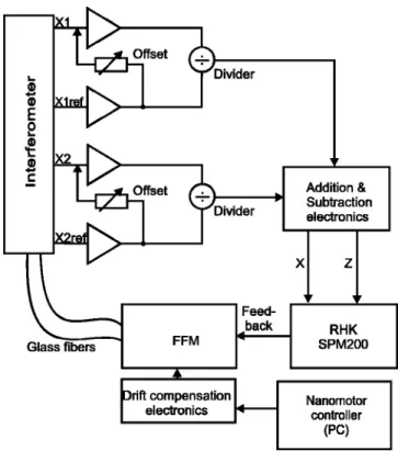
As discussed in Sec. II A, the signal coming from each interferometer consists of a sinusoidal interference compo-nent plus an offset, which is due to the difference in reflec-tion amplitudes. In our detecreflec-tion electronics, we first subtract a fraction of the reference signal and amplify only the inter-ference component. The amplified signal is then divided by the reference signal to reduce the effect of fluctuations in laser diode intensity. The four resulting signals are then added and subtracted according to Eq. 共4兲 to produce the three-dimensional Tribolever displacement information. All signals are then used as input for an RHK SPM200 system with added input capabilities so that the fully three-dimensional motion of the tip can be monitored in real time. A common problem in force microscope setups using fiber optic interferometry is drift between the fiber end face and the cantilever due to thermal expansion of the microscope.27 Although we have used materials with low FIG. 5.共a兲Perspective drawing of the microscope assembly.共b兲Side view
with共1兲fiber positioning head,共2兲XY motor,共3兲Z coarse approach motor,
共4兲kinematic mount between the motor/sample stage and the fiber position-ing head.
FIG. 6. Block diagram of the microscope’s electronics共shown again only for the X pair兲. From the X1 and X2 signals coming from the interferometer an adjustable fraction of the reference signal is subtracted before the first amplification. The result is divided by the reference signal. This procedure allows the maximum amplification of the signal while introducing the low-est noise level. In the addition and subtraction electronics, the outputs from the X1 and X2 dividers are combined according to Eqs.共2兲–共4兲in order to obtain voltages that correspond to the true displacement of the Tribolever共X and Z兲. These voltages are then fed into a commercial scan electronics system, which acquires the measured data and controls the sample motion
共scanning and feedback兲.
thermal expansion coefficients for the fiberhead components, the fiber-pyramid distance drifts slowly due to temperature variations in our nonclimatized laboratory. Using home-built electronics we apply very slow voltage ramps to the Nano-motors®, to keep the fiber-pyramid distance constant for sev-eral hours.
E. Calibration
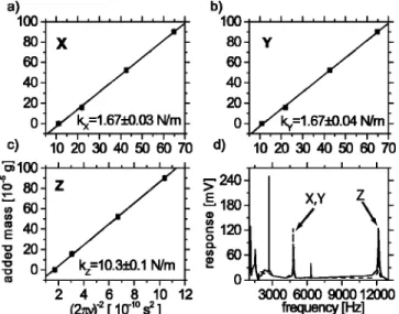
One of the extreme advantages of the Tribolever® is that it allows easy, yet very precise calibration. We routinely cali-brate each Tribolever® prior to its first use. By exciting the Tribolever® acoustically with a loudspeaker, that is placed close to the fiberhead, frequencies of the resonances in the X, Y and Z directions can be measured. Soda lime glass beads28 with masses ranging from 1.57 to 9.01g have been placed on the central cross of the pyramid. By measuring the reso-nance frequencies as a function of the added mass, extremely accurate values of the Tribolever’s® lateral and vertical spring constants have been determined.29 Figure 7 is an ex-ample of one such calibration run. This calibration procedure has no effect on the Tribolever® because the sphere is held in place by gravity. Calibration of the lateral 共torsional兲 spring constant on traditional AFM cantilevers is more time consuming, more complex and significantly less accurate.30
Measured lateral spring constants in this example 共Fig. 7兲 are kX=共1.67± 0.03兲N / m and kY=共1.67± 0.04兲N / m. These two spring constants are virtually identical and they are close to the value of 1.4 N / m calculated from the dimen-sions of the legs of the Tribolever® using finite element analysis. The measured vertical spring constant for the Tri-bolever® is kZTribolever=共10.3± 0.1兲N / m as compared to the calculated value of 25.8 N / m. The large deviation is due to the additional flexibility of a thin diaphragm 共2 mm
⫻2 mm⫻10.6m兲 that supports the Tribolever® on the silicon chip. This diaphragm is the result of a wet etch step
that forms a wide, recessed window to allow room for the detection fiber’s access to the pyramid共Fig. 1兲.
In the design of the Tribolever® device the geometry of window was changed to overcome this problem.
We also used the resonance spectra of the Tribolever® to estimate the noise levels of the optical detection and the elec-tronics. With a spectrum analyzer, we measured the ther-mally excited X and Y resonances of a Tribolever® with lateral spring constants of 5.75 N / m. The amplitude of the resonant motion can be calculated by the equipartition theo-rem 21kxxrms
2 =1
2kBT, where xrmsis the root mean square
ther-mal motion amplitude, kBis the Boltzmann constant and T is the temperature. If the electronic instrument noise is much smaller than the thermal motion of the sensor, the root mean square voltage noise Vrmsat the resonance frequency is given
by the relation␣Vrms= xrms=
冑
kBT / kx.31␣is a known calibra-tion factor that relates the output voltage to the displacement of the Tribolever®. We compared the measured Vrmswith thecalculated value of Vrmsat the thermal limit. We found that
the detected noise in the frequency range of the lateral reso-nances 共9.38 kHz兲 is a factor of 1.9 共X1兲–4.8 共Y2兲 higher than the thermal noise. In a FFM measurement, the noise levels are certainly different. Typical signal frequencies are lower共below 2 − 3 kHz兲and the tip is in contact with a sur-face. However, the measured noise levels provide a good indication that the detection is operating close to the thermal limit, which is confirmed by test measurements on a graphite sample共see next section兲.
The differences in the noise levels between X and Y might be due to specific details of the interferometer branches共especially the quality of connectors and of the end face of each fiber兲. We assume that the signal to noise ratio can be further improved by coating the fiber end faces with a metal layer to increase the reflectance of the fiber/air inter-face共see Sec. II B兲.
III. EXPERIMENTAL RESULTS
For a first testing of the instrument and the complex data acquisition we used a commercial AFM calibration sample with a regular ripple structure of known dimensions.32 The employed sample is a glass substrate that has parallel alu-minium hills with a period of 278± 1 nm and a height ex-ceeding 30 nm. The tip was electrochemically etched from a tungsten wire and glued into the Tribolever®. Figures 8共a兲–8共c兲show topography and friction images that were re-corded simultaneously at a constant normal load of 0.85 nN. The topography image shows the parallel hill-and-valley structure of the calibration sample. The height of the hills is 33 nm. The friction force images show high frictional forces on top of the aluminium stripes both in X and Y direction plus an additional lateral force, where the tip ran against the stripes. A plot of a scan line in the forward and in the back-ward direction of image 8共b兲 shows a typical friction loop. When the ridges are aligned perpendicular to the X direction, the maximum friction force measured in the X direction is a factor 200 higher than the maximum friction force that is measured in the Y direction, which shows that the coupling between X and Y directions is at most 0.5%.
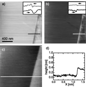
As a second test sample we used a highly oriented py-rolytic graphite 共HOPG兲 surface. Figure 9 depicts lateral force maps measured in the forward X direction and Y direc-tion 共a,b兲 and the topography map 共c兲 of two graphite ter-races separated by a 0.3-nm-high step. Because of the much higher spring constant in the normal direction the topo-graphic image shows less detail than the lateral force map. As has been reported in several previous articles共e.g. Ref. 33兲the lateral force at the step edge is enhanced when the tip is moving step up and also step down.
Figure 10 shows friction forces measured in the X direc-tion共open circles兲and in the Y direction共open squares兲 on an atomically flat graphite terrace as a function of the sliding angle. To obtain the friction force in the sliding direction
共closed circles兲 the vector addition of the friction forces in the X and the Y direction needs to be computed
FF= FXFcos+ FYFsin, 共5兲
where denotes the angle between the X direction of the Tribolever and the sliding direction of the tip. Whereas the measured friction force in the X and the Y direction varied strongly with the sliding direction, the friction force in the sliding direction stayed nearly constant as expected from a Tomlinson model calculation. This demonstrates the capabil-ity of the microscope to measure friction forces in any slid-ing direction.
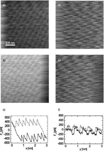
The three-dimensional force sensitivity at the atomic scale is demonstrated in Fig. 11. Panels共a兲,共b兲,共d兲,共e兲show forward and backward friction maps with the HOPG sample in X and Y direction of a 3-nm⫻3-nm-wide area. The
mea-surement was performed in a scan direction, which was not aligned along either the X or the Y direction of the Tri-bolever, and atomic scale variations in the friction force could be observed in two directions. The friction loops show a “sawtooth-like” signal for the X direction关Fig. 11共c兲兴and a “square-wave”-like signal for the Y direction 关Fig. 11共f兲兴. From these signals it can be deduced that the tip follows a “zig-zag” trajectory on the graphite lattice.34 It is important FIG. 8. Simultaneously measured topography and lateral force images of a
TDG01 calibration sample. 共a兲 Topography 共feedback兲 image. The gray scale corresponds to 39.8 nm,共b兲lateral force image in the X direction. The gray scale corresponds to 115 nN,共c兲lateral force image in the Y direction. The gray scale corresponds to 258 nN,共d兲friction loop formed by a forward
共solid兲and backward共dashed兲scan line measured in the X direction. The image size is 1.5m⫻1.5m and the constant normal force is FN
= 0.85 nN.
FIG. 9. Correlation between lateral force and topography images of a step running across a HOPG sample.共a兲Lateral force image in the forward X direction.共b兲Lateral force image in the forward Y direction. The insets in
共a兲and 共b兲 show line scans in the forward共black兲 and in the backward direction共gray兲, as indicated by a line in both images. The lateral force at the step is enhanced, both in the upward and the downward direction. Note also that the force response of the step is different in the X and the Y direction. The lateral force scale of the insets corresponds to 300 nN.共c兲 Simultaneously measured topography image,共d兲line scan of the topography image.
FIG. 10. Friction force on an atomically flat HOPG surface as function of the sliding angle. The open circles denote the friction FX
Fmeasured in the X
direction of the Tribolever, the open squares the friction FY F
in the Y direc-tion. The closed circles show the friction FFin the sliding direction
calcu-lated from these components, according to Eq.共5兲. The dashed lines are a sine and a cosine fit to the friction components in the X and the Y direction. The dotted line shows calculated friction forces, obtained using a Tomlinson model.
to note that the lateral forces measured with our microscope are much lower than in previous studies共e.g. Ref. 35兲. From the noise in the X and Y channels during the friction mea-surements, we estimate that the lateral force resolution共rms兲 in the measurement is 15 pN in the X direction and 41 pN in the Y direction. The topography image共not shown兲does not show any structure, although the feedback system had been set for constant normal force. This implies that the topogra-phy and friction signals are completely decoupled.
ACKNOWLEDGMENTS
The authors gratefully acknowledge H. J. Hug from the University of Basel who helped develop and adapt the sample manipulation motors. This work is part of the re-search program of the “Stichting voor Fundamenteel Onder-zoek der Materie共FOM兲” and was made possible by finan-cial support from the “Nederlandse Organisatie voor Wetenschappelijk Onderzoek共NWO兲.”
1
D. Dowson, History of Tribology, 2nd ed.共Longman, London, 1998兲.
2
I. L. Singer, R. N. Bolster, J. Wegand, S. Fayeulle, and B. C. Stupp, Appl. Phys. Lett. 57, 995共1990兲.
3
U. D. Schwartz, O. Zwörner, P. Köster, and R. Wiesendanger, in Micro/ Nanotribology and Its Applications NATO ASI Series E Vol. 330, edited by B. Bhushan共Kluwer, Dordrecht, 1997兲, p. 233.
4
J. Greenwood, in Fundamentals of Friction: Macroscopic and Micro-scopic Processes, NATO ASI Series E Vol. 220, edited by I. L. Singer and H. M. Pollock共Kluwer, Dordrecht, 1992兲, pp. 37–56.
5
B. Bhushan, J. Israelachvili, and U. Landman, Nature共London兲 374, 607
共1995兲.
6
R. W. Carpick, N. Agraït, D. Ogletree, and M. Salmeron, J. Vac. Sci. Technol. B 14, 1289共1995兲.
7
P.-E. Mazaran and J.-L. Loubet, Tribol. Lett. 3, 125共1997兲.
8
D. F. Ogletree, R. W. Carpick, and M. Salmeron, Rev. Sci. Instrum. 67, 3298共1996兲.
9
U. D. Schwarz, P. Köster, and R. Wiesendanger, Rev. Sci. Instrum. 67, 2560共1996兲.
10
T.-Y. Fu, Y.-R. Tzeng, and T. T. Tsong, Surf. Sci. 366, L691共1996兲.
11
T. Zijlstra, J. A. Heimberg, E. van der Drift, D. Glastra van Loon, M. Dienwiebel, L. E. M. de Groot, and J. W. M. Frenken, Sens. Actuators, A
84, 18共2000兲.
12
ANSYS©, finite element analysis software, Ansys, Inc., Canonsburg, PA.
13
U. Rabe, K. Janser, and W. Arnold, Rev. Sci. Instrum. 67, 3281共1996兲.
14
G. J. Germann, S. R. Cohen, G. Neubauer, G. M. McClelland, and H. Seki, J. Appl. Phys. 73, 163共1993兲.
15
A. Moser, H.-J. Hug, Th. Jung, U. D. Schwarz, and H.-J. Güntherodt, Meas. Sci. Technol. 4, 769共1993兲.
16
D. Rugar, H. J. Mamin, and P. Guethner, Appl. Phys. Lett. 55, 2588
共1989兲.
17
Components of the interferometer are: Laser diode: Sony, gain-guided SLD 201 V-3, = 780 nm,S / N = 80 dB at maximum 2.5 mW output coupled directly to Faraday isolator and fiber pigtail with an angled pol-ished FC connector 共FC/APC兲 at the output end. Current source: ILX Lightwave, battery controlled LD-2000,⬍800 nA rms noise, 5 ppm long term共1 – 20 h兲stability. Thermal electric cooler, TEC TC-5100, and high power heat sink from ILX Lightwave, Bozeman, MT. Glass fibers and couplers: Wave Optics, Inc., Hillsboro, OR single-mode, mode field diam-eter 5.5m, cladding diameter 125m, numerical aperture 0.11, termi-nated with FC/APC connectors
18
Methods developed for making sharp near-field scanning microscopy tips cannot be used in our application because they stretch the core and de-crease its diameter as it is melted. This would introduce spurious backre-flections into our interferometer.
19
Wave Optics, Inc., Mountain View, CA.
20
D. R. Turner, US Patent No. 4,469,554共1983兲.
21
P. Hoffmann, B. Dutoit, and R.-P. Salathé, Ultramicroscopy 61, 165
共1995兲.
22
Nanomotor®, Klocke Nanotechnik GmbH, 52078 Aachen, Germany.
23
This idea was first used by Olaf Wolter in the alignment chip共ALIGN兲 from Nanosensor GmbH producing repositioning resolutions of 5m. However, the ALIGN systems of ridges and grooves do not form a true kinematic mount. In theory, a trihedral hole is required to form a true kinematic mount. Due to the wet etching characteristics of silicon, a quad-rahedral hole is used with very nice results.
24
Staveley NDT Technologies, Inc., EBL 2 piezo tube, outer diameter 0.25 in., length 0.5 in., wall thickness 0.03 in..
25
H.-J. Hug, B. Stiefel, P. J. A. van Schendel, A. Moser, S. Martin, and H.-J. Güntherodt, Rev. Sci. Instrum. 70, 3625共1999兲.
26
M. Dienwiebel, G. S. Verhoeven, N. Pradeep, J. W. M. Frenken, J. A. Heimberg, and H. W. Zandbergen, Phys. Rev. Lett. 92, 126101共2004兲.
27
R. Euler, U. Memmert, and U. Hartmann, Rev. Sci. Instrum. 68, 1776
共1997兲.
28
Dragonite® glass beads, Jaygo Inc., Union, NJ.
29
J. P. Cleveland, S. Manne, D. Bocek, and P. K. Hansma, Rev. Sci. Instrum. 64, 403共1993兲.
30
D. Ogletree, R. W. Carpick, and M. Salmeron, Rev. Sci. Instrum. 67, 3298
共1996兲.
31
R. D. Grober et al., Rev. Sci. Instrum. 71, 2776共2000兲.
32
TDG01 diffraction grating, NT-MDT Co., Moscow, 103460, Russia.
33
T. Müller, M. Lohrmann, T. Kässer, O. Marti, J. Mlynek, and G. Krausch, Phys. Rev. Lett. 79, 5066共1997兲.
34
S. Fujisawa, K. Yokoyama, Y. Sugawara, and S. Morita, Phys. Rev. B 58, 4909共1998兲.
35
C. M. Mate, G. M. McClelland, R. Erlandsson, and S. Chiang, Phys. Rev. Lett. 59, 1942共1987兲.
FIG. 11. Lateral force maps for a W tip on HOPG moving in the X direc-tion. Lateral forces in the X direction共a兲 forward scan. The gray scale corresponds to 1.4 nN,共b兲backward scan. Gray scale: 1.5 nN,共c兲friction loop. Lateral force map in the perpendicular Y direction:共d兲forward scan. Gray scale: 222 pN,共e兲 backward scan. Gray scale: 243 pN,共f兲 friction loop. All images were measured simultaneously with FN= 35.8 nN; image