SUPPLEMENT SERIES
Astron. Astrophys. Suppl. Ser.137, 75–81 (1999)
ESO Imaging Survey
?
IV. Multicolor analysis of point-like objects toward the South Galactic Pole
S. Zaggia1,2, I. Hook1, R. Mendez1,3, L. da Costa1, L.F. Olsen1,4, M. Nonino1,5, A. Wicenec1, C. Benoist1,6,
E. Deul1,7, T. Erben1,8, M.D. Guarnieri1,9, R. Hook10, I. Prandoni1,11, M. Scodeggio1, R. Slijkhuis1,7, and
R. Wichmann1,12
1 European Southern Observatory, Karl-Schwarzschild-Str. 2, D–85748 Garching b. M¨unchen, Germany 2
Osservatorio Astronomico di Capodimonte, via Moiariello 15, I-80131 Napoli, Italy 3 Cerro Tololo Inter-American Observatory, Casilla 603, La Serena, Chile
4
Astronomisk Observatorium, Juliane Maries Vej 30, DK-2100 Copenhagen, Denmark 5 Osservatorio Astronomico di Trieste, Via G.B. Tiepolo 11, I-31144 Trieste, Italy 6
DAEC, Observatoire de Paris-Meudon, 5 Pl. J. Janssen, F-92195 Meudon Cedex, France 7
Leiden Observatory, P.O. Box 9513, 2300 RA Leiden, The Netherlands
8 Max-Planck Institut f¨ur Astrophysik, Postfach 1523, D-85748 Garching b. M¨unchen, Germany 9
Osservatorio Astronomico di Pino Torinese, Strada Osservatorio 20, I-10025 Torino, Italy
10 Space Telescope – European Coordinating Facility, Karl-Schwarzschild-Str. 2, D–85748 Garching b. M¨unchen, Germany 11
Istituto di Radioastronomia del CNR, Via Gobetti 101, I-40129 Bologna, Italy 12 IUCAA, Post Bag 4, Ganeshkhind, Pune 411007, India
Received July 17; accepted December 16, 1998
Abstract. This paper presents preliminary lists of
poten-tially interesting point-like sources extracted from multi-color data obtained for a 1.7 square degree region near the South Galactic Pole. The region has been covered by the ESO Imaging Survey (EIS) in B, V and I and of-fers a unique combination of area and depth. These lists, containing a total of 330 objects nearly all brighter than
I ∼ 21.5, over 1.27 square degrees (after removing some bad regions), are by-products of the process of verifica-tion and quality control of the object catalogs being pro-duced. Among the color selected targets are candidate very low mass stars/brown dwarfs (54), white-dwarfs (32), and quasars (244). In addition, a probable fast moving as-teroid was identified. The objects presented here are nat-ural candidates for follow-up spectroscopic observations and illustrate the usefulness of the EIS data for a broad range of science and for providing possible samples for the first year of the VLT.
Key words: surveys — quasars: general — while
dwarfs — stars: low-mass
Send offprint requests to: M. Nonino
? Tables 2 to 8 are only available in electronic form at the
CDS via anonymous ftp to cdsarc.u-strasbg.fr (130.79.128.5) or via http://cdsweb.u-strasbg.fr/Abstract.html
1. Introduction
The present paper is the fourth of a series presenting the data accumulated by the public ESO Imaging Survey (EIS), being carried out in preparation for the first year of regular operation of the VLT. As described in previ-ous papers (Renzini & da Costa 1997; Nonino et al. 1998, hereafter Paper I) the main goals of the EIS project are to conduct an imaging survey suitable for finding “rare” objects for follow-up observations with the VLT and to lay down the groundwork for more ambitious wide-field digi-tal, multicolor imaging surveys. The adopted strategy was designed to search for distant clusters of galaxies, quasars, high-redshift galaxies and to identify rare stellar types.
comparisons indicates that the available data, reduction procedures and object catalogs extracted in each of the passbands are reliable. Furthermore, comparison of the observed color distribution for point-like sources, derived from a preliminary version of a color catalog, with predic-tions of galactic models also shows reasonable agreement. Although encouraging, the above results do not fully characterize the color catalog, in particular if it is to be used to identify different types of objects based on color selection criteria. Target selection based on the location of objects in color-color space, require a careful investigation of the performance of the pipeline since any problem may lead to objects with spurious colors. Colors are sensitive to a number of effects such as the observing conditions, the photometric and astrometric solutions in the different passbands and the de-blending algorithm. In order to have a better understanding of the impact of these effects in the color catalog, in this paper the (B−V) versus (V−I) diagram for point-sources is used to select objects lying in potentially interesting regions of the color-color space; such regions have been defined following by an appropri-ate modelling of the expected colors of such interesting objects. The objects, examined individually, are used to generate lists of candidates for different type of objects.
The goals of the present paper are: 1) to test the per-formance of the EIS pipeline in the production of object catalogs; 2) to assess the reliability of the color catalogs being extracted from the EIS multicolor data; 3) to pro-vide ESO users with lists of potential VLT targets.
In Sect. 2, the basic characteristics of the color catalog relevant to the present work are described. In Sect. 3, the color-color diagram for point-like sources is inspected and empirical color criteria are used to generate a preliminary list of candidate white-dwarfs, low mass stars and quasars, with a range of red-shifts. Results and the outlook for the future is presented in Sect. 4.
2. The point-source color catalog
The color catalog described here has been constructed from objects detected in the 150 s exposures using multi-color data presented in Paper III. Color catalogs extracted from the co-added images will only be available in the final release.
As discussed in Paper III, the generation of a color cat-alog for generic use is a complex task given the range of possibilities in its definition, which depends to a large ex-tent on the science goals. Since the inex-tention of the present paper is primarily to understand some general characteris-tics of the color catalog and evaluate its usefulness for the primary science goals of the survey, the following prescrip-tion has been adopted. Starting from the unique catalogs covering the whole patch extracted from the best available images in each passband (see Paper III), a color catalog is created by associating the objects detected in the differ-ent passbands (see Paper I). The final product is a unique
entry for each object, listing the photometric parameters and flags for each detection in each passband, and infor-mation about the best seeing frames in all bands. This information allows limits on the color for objects not de-tected in some of the passbands to be calculated. At this point all detections are considered, regardless of the band in which they were detected and the nature of the object (star/galaxy).
It has been found, for instance, that this catalog con-tains objects detected in the blue passbands without coun-terparts in V and I. Visual inspection of some of these cases, which represent roughly 2% of the total number of objects for B <∼22, shows that the unusual colors ob-served come mostly from objects detected at the border of individual frames or along diffraction spikes of bright stars. Others are due to ghost images present in theBand
V images (see Paper III) and to merged images that are de-blended in some passbands and not in others, depend-ing on the seedepend-ing. Even though this is the most general color catalog, it is not the most convenient catalog to use. This is especially the case for extended objects for which are contaminated by the problems mentioned above and for which one would like to have the object centroid and measure magnitudes with the same aperture in all bands. Another problem is that the star/galaxy classification may vary from band to band, thus implying that the object classification may not be unique.
To avoid some of these ambiguities, this paper con-siders only point-sources as defined in the I-band where image quality is more homogeneus than in other bands and it was preferred to theV-band (where image quality is slightly better Figs. 1 and 3 of Paper III), for consistency with the other patches and because the interest is mainly red objects. The selected sample includes only objects de-tected in the I-band brighter than I = 23.0 and with SExtractor stellarity index ≥ 0.75. In addition, all ob-jects with non-zero SExtractor and WeightWatcher flags (Paper I) are removed from the catalog, in order to min-imize contamination by spurious extreme color objects, which originate from some of the cases described above. It is worth pointing out that by eliminating all these ob-jects a priori may discard some interesting cases. The final sample is available athttp://www.eso.org/eis/.
Note that star/galaxy classification is only reliable for magnitudes brighter than I∼21.5 and colors were com-puted using the mag auto estimator introduced in Paper I. The mean error in the colors are less than 0.15 mag for sources brighter than the star-galaxy separation limit, and about 0.4 mag near the limiting magnitude of the sample. Since the primary goal of this paper is to illustrate the possible use of EIS data for different science goals and to evaluate the size of interesting samples for follow-up work, the criteria adopted have been in general conservative. In particular, in the selection of targets discussed below only reliableI-band detections, with the error (I) on the
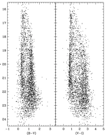
Fig. 1.Color-magnitude diagrams for EIS point-like sources
Furthermore, to avoid regions of very poor seeing and low transparency, some regions were discarded, based on the distributions of seeing and limiting isophothes shown in Paper III, leading to a sample covering a total area of 1.27 square degrees (e.g., Fig. 4). In particular, it was ex-cluded the region withα >12◦.75,δ >−29◦.5 whithBand
I-band seeing>100.3, and the region 12◦.10< α <11◦.90,
δ < −29◦.75 with limiting isophote in I-band <∼25 (very poor transparency).
To illustrate the general properties of the sample the color-magnitude diagramsV versus (B−V) andV versus (V −I) are shown in Fig. 1 for 3233 point-sources with
S/N & 5 in the I passband. The color distribution for sources brighter than V = 21 has already been discussed in Paper III and compared with model predictions. This plot is presented inV-band to make the comparison with other works easier (e.g., Reid & Majewski 1993). Note that at faint magnitudes (V &21.5) incompleteness in the stellar sample sets in (see Paper III). In the figure blue, (B−V)∼0.5, and red, (B−V)∼1.5 concentrations are clearly seen forV &18.5. This reflects the typical bimodal color distribution observed for faint stars at high-galactic latitude, with the blue peak arising from the turnoff of the main sequence for low-metalicity halo stars and the red peak from disk stars. Note that the blue peak is well-defined in the magnitude range 18.5 < V < 21.5.
For fainter magnitudes it fades away partly due to the incompleteness of the catalog and partly because at this magnitude limit one is approaching the outer parts of the halo.
From the figure one sees that for V & 19 there is a large number of objects bluer than the concentration as-sociated with the halo stars, and for V &21.5 there is a population of very red objects with (V −I)>3.5. Both are examples of interesting populations, the identification of which is better explored using the color-color diagram as discussed in the following section.
3. Target selection
Figure 2 left panel shows the color-color diagrams for the 3233 point sources detected simultaneously in the B, V
and I band with (S/N)I & 5; Fig. 2 right panel shows the 345 objects only detected in V and I and not in
B-band with (S/N)I & 5. The plots include all objects brighter than I = 23. For non-detections in B (here-after B-dropouts) an estimate of the B limiting magni-tude has been measured on the best seeing frame. The limiting magnitude is defined to be a 1σdetection within the area corresponding to the seeing-disk as measured in theI-band. From this an estimate of the lower limit on the (B−V) color is calculated. In addition to theB-dropouts, there are objects only detected in the I-band, for which the lower limit in (V −I) is similarly computed. While a large number of these objects is expected if one considers the sample as a whole (because of the relative bright lim-iting magnitudes of the V images), objects brighter than
I ∼21 are the most interesting and are the ones consid-ered in more detail below.
Fig. 2.Color-color diagram for EIS point-sources. Left-panel: those detected in all three passbands. Right-panel: those detected inV andI but notB, for which the lower limit in (B−V) is indicated
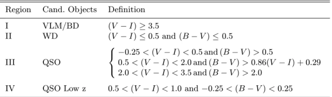
Table 1.Definition of regions of interest in Fig. 3 for candidate objects Region Cand. Objects Definition
I VLM/BD (V −I)≥3.5
II WD (V −I)≤0.5 and (B−V)≤0.5
III QSO
−0.25<(V −I)<0.5 and (B−V)>0.5
0.5<(V −I)<2.0 and (B−V)>0.86(V −I) + 0.29 2.0<(V −I)<3.5 and (B−V)>2.0
IV QSO Low z 0.5<(V −I)<1.0 and−0.25<(B−V)<0.25
filters (Paper I). The method is the same as that used by Warren et al. (1994) and Hall et al. (1996), and is a modified version of the method of Warren et al. (1991). QSO spectra were synthesised assuming that the QSO continuum has the form of a single power law with spectral indexα(S(ν)∝να) and assuming fixed emission line strengths relative to Lyα +N V. Three different values of the spectral index α = (−0.25,−0.75,−1.25) were used, and three different values for the emission line strength, defined by the Lyα + N V rest-frame equivalent width, EW(Lyα+N V) = (42, 84 and 168 ˚A). For each set of assumptions, spectra were generated at intervals of 0.1 in z over the range (3.0 < z < 5.0). Absorption by intervening HI was taken into account by simulating absorption spectra, following the method of Warren et al. (1994) and based on the work of Møller & Jacobsen (1990). For each set of intrinsic properties, ten QSO spectra were generated at each z step, each using a different realization of the absorption spectrum appropriate for that redshift. Thus at each redshift a total of 90 spectra were generated. Because patch B is close to
the South Galactic Pole galactic extinction was neglected in the present calculation. Figure 3 shows the median and the scatter corresponding to the various simulations as a function of redshift.
In addition, in Fig. 3 all the 19 known quasars present in the field are shown in their measured EIS magnitudes. These quasars have redshifts, taken from the literature, in the range 0.4< z <2.96.
Fig. 3.Theoretical color-color plot for different type of objects. The solid line shows the location of main sequence, sub- and red-giant branch stars of an old halo, low metallicity, stellar population model taken from Bertelli et al. (1994). The dotted line shows the location of main sequence, sub- and red-giant branch stars of a young disk, solar metallicity, stellar popula-tion model taken from Bertelli et al. (1994). The short-dashed line shows the location of a WD pure Hydrogen cooling se-quence taken from Bergeron et al (1995). The long-dashed line shows the location of 5 Gyr old BD stars with solar metallicity, taken from Baraffe et al. (1998). The color track for QSOs at different redshifts (3.05 < z < 5.00) are shown by triangles while the dots indicate the typical scatter around the median for the different parameters of the spectral properties and ab-sorbers of high-redshift quasars (see text). Also shown (stars) are the EIS colors of the known quasars present in the EIS catalog which have redshifts in the range 0.4< z <2.96
(V−I) color and its error estimateε(V−I); and in Col. (10) notes or comments on the individual objects, whenever necessary. In the cases where the (B−V) and/or (V−I) colors are lower limits, the measure is preceded by a>sign and the error in the color is the error in the magnitude in the passband in which the object is detected. For objects not detected in two passbands the error in the color is set to zero in the tables.
3.1. Rare stellar-type candidates
One of the interesting regions of the color-color diagram is the region redder than (V−I)≥3.5 (region I). Objects in this region extend well beyond the track defined by main-sequence stars with masses greater than 0.6M. Therefore, this region should be populated primarily by
very low mass stars (0.6 > M/M > 0.1) in the disk and/or brown dwarfs. Another possibility is that they are asymptotic giant and red giant branch stars. However, this is unlikely because there should be few of them in this color and magnitude range since they would have to be high metallicity objects at very large distances from the Sun (∼100 kpc). Even though unlikely, considering the size of the area covered by the EIS multicolor data, this region of the color space could also be populated by very high-redshift QSOs with very large (B−V), which could appear as B non-detections. In this region there are 18 detections (listed in Table 2; 22 B-dropouts with (V −I)≥3.5, all brighter thanI= 20 (listed in Table 3); and 14 objects withI <∼21, which are only detected in the
I-band (listed in Table 4). In the tables with “rare” stel-lar objects (2, 3 and 4), the following naming convention has been adopted: VLM, for very low mass candidates, VLMB, for very low massB-dropouts, and VLMI, for the objects only detected in theI-band.
Since extreme colors could be caused by some un-expected artifact all these cases have been visually inspected, and all seem to be legitimate candidates. Note, however, that in the course of the inspection the two brightest objects in this sample exhibited a strange morphology in the coadded image appearing to be a “double” star, with the two objects having almost exactly the same magnitude, I = 17.46±0.01, and a few arcsecs of separation. This prompted the examina-tion of the two single frames, which showed a single slightly elongated object that occupies different positions in the two single exposure images. The object was observed at α = 00h49m37s.71, δ = −29◦5005800.7, JD = 50696.3174202 and α = 00h49m37s.76,
δ = −29◦5005600.7, JD = 50696.32054438. This fact strongly suggests that this object is probably a relatively fast moving asteroid. However, no known asteroids were found to be at the observed position during the nights the observations were conducted. This example of a serendip-itous source demonstrates the need to implement tools in the EIS pipeline to search for transient phenomena present in the survey such as high proper-motion objects, variables, supernovae.
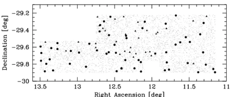
Fig. 4.Projected distribution of star-like objects which shows: all stellar objects detected in the selected area of patch B (dots); low-mass candidates found in region I of the color-color diagram of Fig. 3 (filled circles); and WD candidates in re-gion II (filled triangles)
objects. As can be seen from Fig. 3, this sample can be contaminated by low redshift quasars. In fact Table 5 contains 2 already known quasar which are identified (name and redshift from the Simbad database). The U -band data will be useful to sort out these cases.
Finally, Fig. 4 shows the spatial distribution of these various candidates. Note that the northeast edge of the patch has been removed because of the incompleteness of theB-band catalogs. Similarly, a region along the south-ern edge was removed because of the incompleteness in theI-band catalog. A small trimming of the whole region has also been done yielding a total area of 1.27 square degrees.
3.2. Quasar candidates
From simulations of QSO tracks (Fig. 3) high redshift QSOs (3 < z < 5) can be found in region III of the color-color diagram, while the available sample of known low redshift QSOs populate region IV (see Fig. 3, Osmer et al. 1998). The rough criteria used to define region III (Table 1) were chosen based on the simulated QSO track. The blue part was chosen to be parallel to the stellar lo-cus but shifted to minimize the contamination by stars. Several improvements in the selection can be made to take into account the errors in colors, as a function of the mag-nitude, and to optimize the yield based on the expected density of objects of different types. Since the parent sam-ple is public, interested groups are likely to make signif-icant refinements to the selection criteria adopted here.
In region III there are 70 objects detected in all three passbands. These are listed in Table 6. In addition, there are 126 objects that are detected inV andI but not de-tected inB(hence have lower limits in (B−V)) that could also lie in region IV. These objects are listed in Table 7. Note that, since the depth of the B images varies across the patch, the limits on (B−V) are more meaningful in some areas than others. The depth of the B frames
cor-Fig. 5.Projected distribution of quasar candidates at low (filled circles), intermediate and high redshift (filled triangles). The adopted selection criteria are discussed in the text
responding to each object can be calculated from the V
magnitude and the (B−V) limits given in Table 6. In the tables the following naming convention has been adopted: QSO and QSOB stand for objects in region III detected in all three bands (& 3.0) and B-dropouts candidates, respectively.
Adopting the criteria given in Table 1 for region IV, where QSOs withz <∼3 are likely to be found, one finds 48 stellar objects which are listed in Table 8. This table in-cludes 6 known QSOs, as indicated (name and redshift are from the Simbad database). In the table QLZ stands for low redshift (z <∼3.0) quasars. Note, however, that with the follow-up observations in U-band to be carried out later this year, it will be possible to select low-z QSOs more efficiently.
Figure 5 show the projected sky distribution of the QSO candidates. This figure should be compared with those for the seeing and the limiting magnitudes presented in Paper III to investigate possible correlations between the QSO candidates and the quality of the data, especially the B-dropouts or those detected only in theI-band. At first glance there is no obvious correlation as the QSO can-didates seem to be uniformly distributed over the surveyed area.
4. Summary
defined. It is important to emphasize that in addition to providing these preliminary lists, the present work has been an essential part in understanding the characteristics of the color catalogs being produced and for the verifica-tion of their reliability.
Improvements in the sample selection are certainly possible. The combination of Galactic models, stellar evo-lution, quasar properties and an appropriate modelling of the observational errors in principle can lead to the def-inition of some probability function that can be better used to identify interesting objects; another way can be a direct fit to the broadband spectral emission of the ob-jects. This is beyond the scope of this paper and since the data are publicly available, interested groups may refine the selection criteria and produce their own samples. The present results lead to samples that are of the order of 50 to 100 candidates each. The yield will only be defined by follow-up spectroscopic observations. Much larger samples will be available from the Pilot Survey to be carried out with the new Wide Field Imager at the 2.2 m telescope at La Silla.
Finally, it has been comunicated that observations per-formed at the 2dF of a sample of bright QSO candidates presented in this paper resulted in an identification of 14 QSO with redshift in the range 1÷2.2 out of 26 candidates with a success rate above ∼50% (S. Cristiani, private communication).
Acknowledgements. We thank all the people directly or indirectly involved in the ESO Imaging Survey effort. In particular, all the members of the EIS Working Group for the innumerable suggestions and constructive criticisms, the ESO Archive Group and the ST-ECF for their support. Special thanks to A. Baker and D. Clements for their con-tribution in the quasar search in the early stages of the EIS
project. We would like to thank S. Warren for helpful com-ments and providing the code for the calculation of the color track for quasars for the EIS filters and I. Baraffe for provid-ing the locus of brown dwarfs in the appropriate passbands. We would also like to thank R. Saglia, B. Boyle, M. Colles and S. Cristiani for comunicating their results before of pub-lication. Our special thanks to the efforts of A. Renzini, VLT Programme Scientist, for his scientific input, support and ded-ication in making this project a success. Finally, we would like to thank ESO’s Director General Riccardo Giacconi for mak-ing this effort possible in the short time available. This research has made use of the Simbad database, operated by the Centre de Donn´ees astronomiques de Strasbourg.
References
Baraffe I., Chabrier G., Allard F., Hauschildt P.H., 1998, A&A 337, 403
Bertelli G., Bressan A., Chiosi C., Fagotto F., Nasi E., 1994, A&ASS 106, 275
Bergeron P., Wesemael F., Beauchamp A., 1995, PASP 107, 1047
Boyle B.J., 1989, MNRAS 240, 533
Hall P.B., Osmer P.S., Green R.F., Porter A.C., Warren S.J., 1996, ApJ 462, 614
Møller P., Jakobsen P., 1990, A&A 228, 299
Nonino M., Bertin E., da Costa L., et al., 1999, A&A 137, 51 (Paper I)
Osmer P.S., Kennefick J.D., Hall P.B., Green R.F., 1999, ApJS 119, 1890
Prandoni I., et al., 1999, A&A (submitted) (Paper III) Renzini A., da Costa L., 1997, The Messenger 87, 23 Reid N., Majewski S.R., 1993, ApJ 409, 635
Warren S.J., Hewett P.C., Osmer P.S., 1994, ApJ 421, 412 Warren S.J., Hewett P.C., Irwin M.J., Osmer P.S., 1991, ApJS