Passive scalar intermittency in random flows

(1)

Passive Scalar Intermittency In Random Flows

by Zhi Lin

A dissertation submitted to the faculty of the University of North Carolina at Chapel Hill in partial fulfillment of the requirements for the degree of Doctor of Philosophy in the Department of Mathematics.

Chapel Hill 2007

Approved by:

Richard M. McLaughlin, Advisor Roberto Camassa, Co-Advisor Jingfang Huang, Committee Member

Peter Mucha, Committee Member

(2)

c

2007

Zhi Lin

(3)

Abstract

ZHI LIN: Passive Scalar Intermittency In Random Flows.

(Under the direction of Richard M. McLaughlin and Roberto Camassa.)

This thesis concentrates on reconstructing the complete probability density function (PDF) for a passive scalar governed by a random advection-diffusion equation using a variety of mathematical tools, primarily from partial differential equations, perturba-tion theory, numerical analysis and statistics. First we present a one-dimensional model which is essentially a random translation of pure heat equation. For some determin-istic initial data, the ensuing scalar PDF and its statdetermin-istical moments can be explicitly calculated. We use this model as a testbed for validating a numerical reconstruction procedure for the PDF via orthogonal polynomial expansion. In this model, the Péclet number is shown to be decisive in establishing the transition in the singularity structure of the PDF which affects the effectiveness of the series expansion, from only one alge-braic singularity at unit scalar values (small Péclet), to two algebraic singularities at both unit and zero scalar values (large Péclet). Next, we study the more complicated, two-dimensional model in which the underlying flow is a random linear shear in one dimension. For planar, Gaussian random initial data, we identify the scalar PDF as an integral representing a conditional mixing of Gaussian probability measures averaged over all realizations of a single random variable, namely, the renormalized L2_{-norm of}

(4)

(5)

Acknowledgments

I think that it is much harder, if not impossible, for me to thank all the people that have helped me here in the United States enough, than to complete this thesis. And I cannot fully describe how many things have changed me, in a positive way, ever since I came here five years ago. For me, it is such a honor and privilege to study and work in this wonderful place, with these wonderful people, during all this time that maybe passed too quickly.

I would also like to express my gratitude to the National Science Foundation for their kind financial support through the grant “Collaborations in Mathematical Geosciences” (ATM-0327906) over the last three years.

I sincerely thank ALL the students and PhD students that I met during my stay here, whether we had heated discussions about mathematics, or they were filled with passion when it came to sharing personal interests.

I would like to bring my warm thanks to all the former and present postdoctoral scholars whom I have worked with: Chung, Hayder, Long, Neil, not only for their help in mathematics, but also for their valuable advice on my personal life and career.

I would like to thank our very efficient and helpful secretaries, for being experts all along in alleviating the cultural differences with which international students usually have a hard time. I am especially grateful to Brenda, Elaine and Janet, for their extraordinary, consistent patience with my repetitious being locked out of my office.

(6)

(7)

List of Figures

2.1 C2n and Its Asymptotic Approximation for x= 0 andβ = 1. . . 26

2.2 Asymptotic Behavior of |C2n| When β >1 . . . 26

2.3 4-Term Chebyshev Reconstructions of the PDF at t = 1 . . . 29

2.4 Reconstructions of the PDF via Different Orthogonal Polynomials . . . 30

2.5 Convergence Rates of Series Reconstructions . . . 31

2.6 4-Term Shifted Chebyshev Reconstructions of the PDF at t = 1 . . . . 31

2.7 Convergence Rates for Different r(ξ) and Qn(ξ) . . . 32

2.8 Comparison Between the Exact PDF (2.5) and MC Simulations. . . 33

2.9 Benchmarking the Monte-Carlo Simulator . . . 34

2.10 The Pointwise Error of the Monte-Carlo Simulated P0,10(ξ) . . . 35

2.11 The Short Time Dynamics of Px,t(ξ): from Gaussian to Ribbons. . . 36

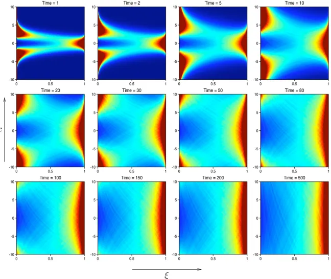
2.12 The Long Time Dynamics of Px,t(ξ): from Ribbons to Stripes. . . 37

2.13 The |x|Value at the “Information Fronts” of VS Time . . . 38

2.14 Effects of the P´eclet number for T0(x) =e−x 2 . . . 39

2.15 The PDF Dynamics of Px,t(ξ) with T0(x) = 2xe−x 2 where Pe = 2 . . . . 42

2.16 The PDF Dynamics of Px,t(ξ) with T0(x) = 2xe−x 2 where Pe = 4 . . . . 42

2.17 “Jump Discontinuity” of Px,t(ξ) with T0(x) = 2xe−x 2 . . . 43

2.18 Monte-Carlo Simulations for Px,t(ξ) withT0(x) = 2xe−x 2 att= 1000 . . 44

2.19 Series Reconstions of P0,t(ξ) with T0(x) = 2xe−x 2 . . . 44

2.20 Short Time PDF Dynamics for T0(x) = e−(x−2) 2 +e−(x+2)2 . . . 46

3.1 The Statistics of η . . . 58

3.2 PDF Evolutions from MC Simulation and Numerical Integration . . . . 59

3.3 PDF Evolutions for Different ˆφ0(k) . . . 60

3.4 PDF Evolutions for Different ˆφ0(k) at the Core . . . 60

3.5 PDF Evolutions for Different ˆφ0(k) Superimposed in Time . . . 61

3.6 Fixed Point PDF Evolutions for Different ˆφ0(k) . . . 62

3.7 Two-Point Correlation Functions for Different ˆφ0(k) . . . 63

3.8 Tail and Core Behavior of the Invariant PDF (3.10) for Different α . . 64

3.9 New Long Time, Invariant Measure in the Diffusionless Limit . . . 67

(12)

5.1 Initial Scalar and Water Thickness Distribution . . . 86

5.2 Initial Velocity Distribution . . . 87

5.3 Scalar Intermittency in Shallow Water Equations. . . 88

(13)

Chapter 1 Introduction

Often referred to as “the last unsolved problem of classical physics”, turbulence is the highly unpredictable, irregular motion that is ubiquitously observed in various fluids in Nature. The modern efforts on attacking this mystery were started by Reynolds with his experiments in 1883, in which he proposed a stability criterion for the transition from laminar to turbulent flows based on the non-dimensional Reynolds number (Reynolds, 1883). Over the last century, the mainstream academic community has come to agree that for turbulent flows, the formidable number of degrees of freedom, and sensitivity to the initial and boundary conditions, warrant a statistical rather than a chaotic yet deterministic characterization. As the culmination of the early stage of turbulence re-search, Kolmogorov advanced the notions of “energy cascade” and self-similarity in his seminal paper (Kolmogorov, 1941), which served as the first statistical theory of tur-bulence. Mathematically elegant as they are, Kolmogorov’s original scaling hypotheses and predictions have been shown to break down within the inertial range by recent anal-yses, experiments and simulations, and numerous efforts have been made to amend and improve those fundamental ideas (Falkovich and Sreenivasan, 2006). Thus, a complete description of turbulence remains a conundrum in science.

This thesis is devoted to an important subject in the study of turbulence: the study

of passive scalars. A passive scalar is a diffusing contaminant immersed in a fluid flow

(14)

mixing properties of the flow fields. Therefore, passive tracer behaviors are critical to our understanding of the key turbulent transport and mixing mechanisms governing the environment in which we live, ranging from as small as human cells, to as large as the atmosphere and the ocean.

In the case of geophysical systems, there has been considerable scientific effort in recent decades attempting to identify the major mixing mechanisms involved in the observed distributions of a variety of tracers over a broad range of temporal and spatial scales. Typically, these distributions exhibit very large and sudden fluctuations and admit non-Gaussian statistics, which is termed“scalar intermittency” . Such observed geophysical and laboratory examples include single point temperature measurements in high Raleigh number convection experiments (Castaing et al., 1989; Ching, 1991) and in high Reynolds number stratified turbulence (Gollub et al., 1991; Thoroddsen and van Atta, 2006), atmospheric wind data (Sreenivasan and Antonia, 1997), and aircraft measurements of stratospheric aerosols (Sparling, 2000). This is inconsistent with the omnipresent Gaussian assumptions in operational meteorology and climatology, due to their mathematical simplicity (Kalman, 1960). And these realistic, scale dependent

probability density functions (PDFs) drastically change the prediction of the state of

the environment as well as of some fundamental changes it might undergo. Therefore, one outstanding problem arises: what are the origins and basic physical mechanisms responsible for generating these non-Gaussian (heavy-tailed) distributions?

(15)

homogenization techniques enable large scale models to provide accurate results that agree with realistic data sets (Grabowski, 2004), without expensive resolution for com-plete, small scale turbulence. However, the highly turbulent feature of many complex systems eliminates such separation in the sense that the active scales of the flow field and those of the tracers overlap. In such cases, traditional treatments may not offer a complete description for the dynamics of the passive tracer fields for which new models and characterizations should therefore be explored.

Subject to appropriate initial and boundary conditions, the evolution of a passive scalar field, T(~x, t), is governed by the advection-diffusion equation:

∂T

∂t +

~

V(~x, t)· ∇T =κ∆T +f(~x, t), ~x∈_R3, t >0 (1.1)

where V~(~x, t) is an incompressible velocity field, κ is the molecular diffusivity of the scalar andf(~x, t) is the external forcing. Such dynamics are linear, but involve random coefficients since the initial condition, the velocity field and the external forcing are all prescribed combinations of deterministic and stochastic components. Consequently, a fundamental question is to predict the inherited statistics (probability measure) of the scalar field which is a complicated interaction between different sources of stochasticity. Nonetheless, this is the simplest scenario to understand the observations of intermit-tency via partial differential equations with random coefficients (Castaing et al., 1989; Chertkov et al., 1995; Chertkov et al., 1997; Chertkov et al., 1998; Kraichnan, 1968; McLaughlin and Majda, 1996; Pierrehumbert, 2000; She and Orszag, 1991; Pumir et al., 1991; Plasting and Young, 2006; Shraiman and Siggia, 1994), which are infinite dimensional systems in finite dimensional spaces. In the case of random passive scalars, such systems have been recognized by the closed evolution equations of the statistical moments in higher dimensional spaces. The linearity of Eq. (1.1) makes such prob-lems tractable, but nonetheless extremely difficult and it is often necessary to appeal to Monte Carlo simulation to gain insight. There are extremely few mathematical analyses on which to base the validity of such simulations.

(16)

for establishing the heavy tail in diffusing passive scalars. This picture is borne out through exact calculations involving the high moment asymptotics for statistical mo-ments of the scalar fields (Bronski and McLaughlin, 2000b; Majda, 1993b), through stochastic analysis (Vanden-Eijnden, 2001), through instanton type field theoretic cal-culations (Chertkov et al., 1998), and through numerical simulation (Holzer and Siggia, 1994; Pierrehumbert, 2000). All of the theoretical calculations have involved highly ide-alized random flow geometries inspired by Batchelor and Kraichnan’s proposition that the turbulent dynamics of small spatial scale passive tracers can be approximated by random but linear straining (Batchelor, 1959; Kraichnan, 1968). In other words, we can

locallywrite the turbulent flow field as V~(~x, t) = A·~x whereA, a random, rank-2

ten-sor representing the principal-rate-of-strain directions and strain parameters subject to incompressibility, can be assumed to be constant over the small scales of interest. Then a class ofsimple shear models(Avellaneda and Majda, 1991; Majda and Kramer, 1999) can be developed, whose simplicity allows rigorous analysis with nontrivial physical relevance. Even in those simplified geometries, only asymptotic information about the PDF tail was available. For these fluid flows which are random shear layers, the scalar is fluctuating either in the presence of a large scale, mean gradient (Bourlioux and Ma-jda, 2002), or in the freely decaying case (Bronski and McLaughlin, 1997; Bronski and McLaughlin, 2000b; Bronski and McLaughlin, 2000a; Bronski, 2003; Majda, 1993a; Ma-jda, 1993b; Majda and Kramer, 1999; McLaughlin and MaMa-jda, 1996; Vanden-Eijnden, 2001). We focus upon the freely decaying scalar case in this thesis.

To understand what is involved with calculating the PDF or the solution of a random PDE, path integrals are generally unavoidable. To see this, consider the evolution of a diffusing passive tracer advected by a general stochastic velocity fieldV~ω(~x, t). Given a

fixed realization ofV~ω(~x, t), the scalarT is uniquely determined by theFeynman-Kac’s

formula:

T(~x, t) =EB[T0(X~B,ω(t))] (1.2)

whereEB is the statistical average over all the pathsX~B,ω(s),0≤s ≤t which satisfies

the stochastic differential equation:

d ~XB,ω(s) =−V~ω(X~B,ω(s), t−s)ds+

√

2κ dB(t), X~B,ω(0) =~x (1.3)

with B(t) as the standard Brownian Motion and κ is the molecular diffusivity of the scalar. Therefore, the PDF for the scalar T conditioned on V~ω is a Dirac measure

(17)

in general, since one has to integrate over all realizations of Vω, namely,

P(T) =

Z

Ω

p(T|V~ω)p(V~ω)dµ(V~ω) =

Z

Ω

δT −EB[T0(X~B,ω(t))]

p(V~ω)dµ(V~ω) (1.4)

where Ω is the space of all realizations of the random velocity fieldV~ω anddµ(V~ω) is the

measure associated to the particular path. When the velocity field admits randomness in both space and time, only very few analyses exist. For example, Kraichnan derived closed evolution equations for statistical moments in rapidly fluctuating fluid flows (white noise limit) (Kraichnan, 1968), and Majda rigorously established, using path integral methods, the general evolution equation governing the N-point correlation function for stationary (in space and time) random shear layers (Majda, 1993b). Also, for scalar fields evolving in an imposed mean scalar gradient (a maintained, large-scale spatially linear scalar profile), Bourlioux and Majda have presented the long time PDF analysis for shear layers with a transverse, temporally varying wind field (Bourlioux and Majda, 2002). For some special cases in which the fluid flows are functionally dependent upon a finite number of stochastic processeswj(t) (Bronski and McLaughlin,

2000a; Bronski and McLaughlin, 2000b; Chertkov et al., 1998; Balkovsky et al., 2001; Majda, 1993b; McLaughlin and Majda, 1996), progress can be made. For example, for fluid flows admitting a linear spatial structure (such as the Majda model which is a linear shear multiplied by temporally varying, Gaussian white noise), an explicit solution to the conditional Feynman-Kac solution in (1.1) is available by the method of characteristics. Even with this explicit, random Green’s function, obtaining the complete probability measure for the random, advected scalar is not possible in general, and requires consideration of the second functional integral in (1.4). Currently, for random, spatially linear fluid flow, existing general results have succeeded in calculating, in closed form, the statistical moments and the PDF tail (Bronski and McLaughlin, 2000a; Bronski and McLaughlin, 2000b; Majda, 1993b; McLaughlin and Majda, 1996; Balkovsky et al., 2001; Vanden-Eijnden, 2001), but not the full measure.

(18)

constant in space, rapidly fluctuating (white in time), Gaussian random advection, we establish here a family of models for which the statistical moments are explicit simple algebraic expressions for any moment number, and for which the complete, explicit, spatio-temporal probability density function is available for specialized initial data. In turn, for more complex initial data, we present a reconstruction procedure based upon orthogonal polynomial expansion, which can approximate the exact PDF very well with a relative error of less than 1% when the first 4 moments are used for the summation, along with high moment number moments asymptotically equal to true moments. Then we use these tools to benchmark Monte-Carlo simulations showing the spatio-temporal evolution of more general PDFs. These calculations give a rigorous and complete demonstration of the role which the P´eclet number, a nondimensional number which measures the relative importance of advection versus diffusion, plays in adjusting the spatial structure of the PDF. Surprisingly, even in this simple flow, the interaction of advection with diffusion is very complicated, and the dynamics smooth in a precise way the initially Dirac scalar distributions for the deterministic initial data. The P´eclet number, the non-dimensional parameter characterizing the relative importance of random advection to molecular diffusion, is shown to move these alge-braic singularities from the diffusion dominated regime, with probability focused at the highest scalar values, to the advective dominated regime, with probability collecting at the zero scalar value. For general models where only moment information is avail-able, the reconstruction procedure is also applicavail-able, provided that the scalar can be renormalized onto a bounded interval.

In Chapter 3, we will discuss the new developments of the simple shear model introduced by Majda in 1993 (Majda, 1993b), which assumed that the velocity field has a simple spatial structure which is a linear shear layer multiplied by a Gaussian white noise process. In this model, theNth _{statistical moment of the tracer may be expressed}

as an explicit N-dimensional integral and this information was used to predict the emergence of heavy-tailed PDFs in previous works. Here, we present new, dynamical behavior for the PDF which occurs within this model by re-formulating the scalar PDF as a conditional mixing of Gaussian probability measures via the law of total probability, whose direct numerical evaluation is non-trivial, since both the conditional variance and the measure of the rescaled L2_{-norm of Wiener Process involved take integral forms.}

(19)

is characterized by an initial growth of the probability density in the core beyond those set by the long time, limiting invariant measure. Simultaneously, the concavity of the PDF is anomalously larger than the invariant measure over several standard deviations. Subsequently, the PDF core in turn decays to the invariant measure. Alternatively, for initial data not possessing a multiply-peaked correlation function, the evolution to the invariant measure is monotonic in the core, and the concavity in the core region is lower than the invariant measure. This behavior we first observed in Monte Carlo simulations, is carefully documented through a more accurate numerical evaluation of an integral representation of the PDF we present. In turn, we identify a new invariant measure which captures this breathing behavior through a distinguished, diffusionless limit. Additionally, we establish that the invariant measure always has a Gaussian core for a wide range of initial cut-off functions, and compute the explicit time scales for the PDF tail to approach the invariant measure. Further, a rigorous analytical prediction of the breathing phenomena is presented for a special class of initial data. Lastly, the partial ergodicity of the model is discussed, where we find that the tracer PDF is semi-ergodic in the sense that the ensemble average over the initial random field can be replaced by its empirical, spatial average.

In Chapter 4, we consider several flows and initial conditions that give rise to explicit random Green’s functions and potentially closed formulas for the scalar statistical mo-ments or even a simple (integral) representation of the full scalar PDF as in the models discussed in Chapter 2 and 3. We seek to extend the methodology to more realistic scenarios and explain the scalar intermittency observed in various experiments.

(20)

and illuminate subsequent analytical efforts.

(21)

Chapter 2 An Elementary Example

In this chapter, we simplified the general governing equation (1.1) by consider the evolution of a decaying passive scalar with a random uni-directional, spatially con-stant wind, for ease in exposition, restricted to one spatial dimension. Then governing stochastic PDE is reduced to

∂T

∂t +γ(t) ∂T

∂x = κ

∂2_T

∂x2, −∞< x <∞, t >0

T|t=0 = T0(x)

(2.1)

whereγ(t) is a Gaussian white noise satisfying

hγ(t)iγ = 0, hγ(t)γ(t0)iγ =σ2δ(t−t0) (2.2)

whereh·iγ denotes the ensemble average over the statistics of γ.

Suppose that the initial data T0(x) has a typical length scale L. Then we have

three dimensional parameters, σ2_, _κ _and _L_{, from which we can only form one}

non-dimensional parameter for Eq.(3.1), the P´eclet number Pe = σ2_/κ_{, that characterizes}

the intensity of the random advection relative to molecular diffusion. If we letx0 =x/L,

τ = tσ2_/L2 _and _γ0₍_τ_{) =} _γ₍_t₎_L/σ2_{, the evolution of the tracer is governed by the}

non-dimensionalized equation

∂T ∂τ +γ

0

(τ)∂T

∂x0 =

1 Pe

∂2T ∂x02

T|τ=0 = T00(x

0

) (2.3)

(22)

is irrelevant here since if we have a different length scale ˜L in the data, then letting ˜

x = x0L/L˜ and ˜τ = τL˜2/L2 will recover exactly the same equation (2.3) but in the variables (˜x,τ˜). This feature is essentially introduced by the vanishing autocorrelation time of the white noise.

This particular time varying fluid flow, while trivial in spatial structure, gives rise to an interesting family of scalar probability measures. These measures give a connec-tion between the respective limits of high and low Péclet number. At zero Péclet (no advection), the solution is trivial, and the ensuing probability measure for the values of the scalar field normalized by the spatial maximum is simply a Dirac mass (delta function) with support set by heat solution (see Result 1, and weak convergence cal-culations below in Section 2.1.5). At the alternative limit, we will see that in the limit of vanishing diffusion the probability measure for renormalized tracer values is also a Dirac mass (delta function) at large times, only with different support set. For finite, non-zero Péclet numbers, the probability measure is a smoother distribution, set by a competition between random advection and diffusion, which we can explicitly compute in this special case to see the connection between these two distributional limits.

The main results for this model are the following: 1. For initial dataT0(x) = e−x

2

, at any fixed locationxand timet, the random scalar

T(x, t) can be renormalized by a deterministic function Tmax(t) = 1/

√

4κt+ 1, so that the ensuingprobability density function (PDF) for ξ :=T(x, t)/Tmax(t) has

compact support, namely,

Prob(ξ /∈[0,1]) = 0 (2.4) Moreover,

(a) The exact spatio-temporal PDF of the renormalized random scalar ξ is

Px,t(ξ) =

r

1

βπ e−x

2

a ξ

1

β−1 _cosh

q −4b0_x2

a2 lnξ

√

−lnξ (2.5)

for any ξ ∈(0,1), where

a= 2σ2t, b0 = 4κt+ 1, β =a/b0 → Pe

2 (t→ ∞) (2.6) This measure has a singular structure at ξ = 1 and if β > 1, x 6= 0, it is also singular at ξ = 0. It converges weakly to the Dirac delta measure δ(ξ) when β → ∞ (high P´eclet number limit for pure random advection) and to

(23)

(b) The Nth statistical moment of the random tracer T(x, t) can be computed analytically as:

hTN(x, t)iγ =

e− N x

2

N a+b0

√

N ab0N−1₊_b0N (2.7)

for N = 0,1,2,· · ·

(c) We formally expand the PDF of the renormalized random tracer by orthog-onal polynomials as

Px,t(ξ) =

P∞

n=0CnQn(ξ)

r(ξ) (2.8)

where{Qn(ξ)}∞n=0 is a family of orthogonal polynomials defined on [−1,1] or

[0,1], r(ξ) is a regularization function and the coefficients Cn are obtained

from the statistical moments of the tracer (2.7). For a specific choice of the polynomial family and r(ξ), the pointwise convergence of these reconstruc-tions depends on the values of x and β. Given the convergence, the fact that P(ξ) is compactly supported by [0,1] guarantees the uniqueness of the expansion. Moreover, with the shifted Chebyshev polynomials, the recon-structed PDF has a relative error of less than 1% when the first 4 moments are used for the summation (2.8).

2. For the bimodal initial data T0(x) = ∂(e

−x2₎

∂x = 2xe

−x2

, T(x, t) can also be renor-malized by Tmax(t) =

√

2e−1_/₍₄_κt _{+ 1), such that Prob(}_{ξ /}∈ _[−₁_,_{1]) = 0. So}

again the probability measure is compactly supported. In this case, the exact, closed-form PDF for the renormalized tracer is available only in a long time limit and it is related to the two branches of the Lambert W-functions(Corless et al., 1997). However, the exact statistical moments of the random tracer T(x, t) are still available at all times in analogy to (2.7). Thus we are able to reconstruct the PDF with orthogonal polynomials as described in Result 1.2.

3. Monte-Carlo (MC) simulations, benchmarked on Result 1, present a detailed picture for the spatio-temporal evolution of the PDF when the exact solution to the moment problem is unknown. The simulation results also illustrate how different values of P´eclet number change the spatial structure of the PDF. Further, simulations are preformed for initial dataT0(x) = 2xe−x

2

andT0(x) =e−(x−A)

2 +

e−(x+A)2

(24)

2.1 Derivation of the Exact PDF and Moments

2.1.1 Exact PDF for

T

₀

(

x

) =

e

−x2

For the unimodal, Gaussian initial data T0(x) =e−x

2

, the exact PDF for the evolving random scalar fieldT(x, t) can be computed analytically via direct statistical inversion, since

T(x, t) = √ 1

1 + 4κtexp

− (x−W(t))2

1 + 4κt

(2.9)

which is a random translation of the pure heat solution, where W(t) = R₀tγ(s)ds is a

Wiener Process(Gardiner, 1985). For example, whenx= 0

Prob(√1 + 4κt T(0, t)≤ξ) = Prob(e−(W1+4(tκt))2 ≤ξ)

= 1−Erf

r

−1 + 4κt

2σ2_t lnξ

(2.10)

where Erf(·) is the error function. Thus, the ensuing probability density function is

P0,t(ξ) :=

∂ ∂ξ

h

1−Erf

r

−1 + 4κt

2σ2_t lnξ i

= ξ

1

β−1

√

−βπlnξ. (2.11)

with β = ₁₊₄2σ2_κtt . To recover the general case (2.5) for x 6= 0, similar but more compli-cated algebra as in Eq.(2.10) is needed. Instead, we follow an alternative derivation using Laplace inversion in Section 2.1.4.

2.1.2 Exact Statistical Moments for General Initial Data

For general initial data, the direct statistical inversion technique shown in Eq.(2.10) is not always applicable, even when an analytic solution similar to Eq.(2.9) is available. However, the exact statistical moments of the random scalar are often accessible. The solution to Eq. (3.1) can be written via Fourier transform as

T(x, t) =

Z ∞

−∞

e2πik[x−W(t)]−4π2κk2t Tˆ0(k)dk (2.12)

where ˆT0(k) is the Fourier transform of T0(x). In fact, this is just a “drifted” version

(25)

hTN(x, t)iγ = h N

Y

j=1

T(xj, t)iγ

=

Z

RN

e2πik·x−4π2κ|k|2tDe−2πiPNj=1kjW(t)

E

γ N

Y

j=1

ˆ

T0(kj)dk

(2.13)

with x= (x1, x2, ..., xN) = (x, x, ..., x) and k= (k1, k2, ..., kN).

Since −2πiPN

j=1kj W(t) is a mean-zero, Gaussian random variable, we have

he−2πiPNj=1kjW(t)i

γ =e−2π

2_σ2_t₍PN

j=1kj)2_. _(2.14)

and Eq. (2.13) reduces to

hTNiγ =

Z

RN

e2πik·x−kTANk

N

Y

j=1

ˆ

T0(kj)dk (2.15)

where

AN =π2



    

a+b a · · · a a a+b · · · a

. . . .

a a · · · a+b



    

(2.16)

with

a= 2σ2t and b = 4κt (2.17)

SinceAN issymmetric positive definite, computing the exact moments is equivalent

to diagonalizing a quadratic form. We start with the special case

T0(x) = δ(x) (2.18)

such that QN

j=1Tˆ0(kj) = 1. The familiar result for a N-dimensional Gaussian integral

reads:

hTN(0, t)i =

Z

RN

e−kTANk_d_k ₌ π N

2

√

detAN

(2.19)

The determinant in the denominator does not vanish providedb6= 0 in Eq. (2.17) and it can be easily shown by induction that detAN = π2N(N abN−1 +bN). For x6= 0, we

(26)

matrix composed ofAN’s eigenvectors and Λ is the diagonal matrix of its eigenvalues

Λ =π2

       

b 0 · · · 0 0 0 b · · · 0 0

. . . . 0 0 · · · b 0 0 0 · · · 0 N a+b

        (2.20)

Changing variables by ¯k=Vk, Eq. (2.15) becomes:

hTN(x, t)iγ =

Z RN e 2πix N P m,n=1 ¯

kmvmn−π2b N−1

P

m=1

¯

k2

m−π2(N a+b)¯k2N dk¯

=

Z ∞

−∞

e2πiVNx¯kN−π2(N a+b)¯k2Ndk¯

N N−1

Y

m=1

Z ∞

−∞

e2πiVmx¯km−π2bk¯2m_d_k¯

m

= π

N

2

√

detAN

e−x2( N−1

P m=1

V_m2

b +

V_N2 N a+b)

= π

−N

2

√

N abN−1₊_bN e

−N x2 N a+b

(2.21)

where Vm = PN_n₌₁vmn, m = 1,2,· · · , N. We will prove Eq.(2.21) by showing Vm = 0

for m < N, VN =

√

N in Appendix. In particular, when x = 0, we retrieve formula (2.19).

To generalize Eq.(2.21) for arbitraryT0(x), we just apply the Convolution Theorem

to Eq.(2.13) and read

hTNiγ =

πN2

√

detAN

Z

RN

exp− 1

b[|y|

2₋ a(

PN

j=1yj)2

aN +b ]

_YN

j=1

T0(x−yj)dy (2.22)

In particular, for T0(x) =e−x

2

, Eq.(2.7) is recovered by computing the above integral, which is the same as in the case of T0(x) =δ(x) except that b is replaced byb0 =b+ 1.

Next we introduce the random variable ξ := _TT(x,t)

max(t) and its N

th_{-order statistical}

moment MN :=hξNiγ and we denote its PDF by Px,t(ξ). Since

MN =

Z ∞

−∞

ξNPx,t(ξ)dξ≥

Z ∞

1

ξNPx,t(ξ)dξ≥

Z ∞

1

(27)

and from Eq.(2.7)

MN =

hTN(x, t)iγ

TN max(t)

= e

− N x2

aN+b0

√

1 +βN →0 (2.24)

asN → ∞, we conclude that

Prob(ξ > 1) = 0 (2.25)

which ultimately leads to Eq.(2.4). This seems redundant here by the simple definition of ξ, while an analogous argument is useful to infer a compactly-supported measure when only the moment information ofξ is available.

2.1.3 Long Time Asymptotics of the Moments

In the long-time limit, we can apply Eq. (2.19) to study the asymptotic behavior of the moments for more general initial conditions and at locations away from the origin. Without loss of generality, we use some of the results from Eq. (2.19) through (2.21) and consider

hTNiγ =

Z ∞

−∞

e2πi

√

N x¯kN−π2(N a+b)¯k2N−π2b N−1

P n=1 ¯ k2 n N Y n=1 ˆ

T0(¯kn)d¯k (2.26)

for an unknown, general T0(x). For a large time t, if we rescale k¯ as k¯ = √k_t, when

t→ ∞,

hTNiγ =

1

√

t

Z ∞

−∞

e2πi

√

N x¯kN−π2(N a+b)¯k2N−π2b N−1

P n=1 ¯ k2 n N Y n=1 ˆ

T(¯kn)dk¯

= √1

t

Z ∞

−∞

e2πi

√

N xkN√

t−π

2N a+b

t k

2

N−π

2b t

N−1

P

n=1

k2n

N

Y

n=1

ˆ

T(√kn

t)dk

∼ √1

t

ˆ

T(0)N

Z

e−π

2N a+b

t k

2

N−π2bt N−1

P

n=1

k2

n

dk (2.27)

= Tˆ(0)N

Z

e−π

2₍_{N a}₊_b_)¯_k2

N−π2b N−1

P

n=1

¯

k2

n d¯k

= Tˆ(0)N π

N

2

√

detAN

provided ˆT0(0) 6= 0 and the quantities a_t and b_t have finite limits as t → ∞, which

(28)

limit, the statistical moments of T are independent of x. To see this, observe that the last two factors in the exponent of the exponential are time-independent constants through Eq. (2.17). Consequently the complex part of the exponential is subdominant at long time. Notice that this asymptotic convergence should be uniform only over compact sets, which will be illustrated in Section 2.4 without a rigorous proof. More importantly, from Eq.(2.27), the tracer field can be renormalized such that the moments of the renormalized tracerξ,hξNi_{, are asymptotically} _self-similar_{, namely, independent}

of both x and t for large times.

2.1.4 Exact PDF and the Inverse Laplace Transform of the

Moment Function

The problem of determining a compactly-supported measureP(ξ)dξfrom its moments is known as theHausdorff Moment Problem. Once the exact moment of arbitrary order is determined, the problem has a unique solution(Shohat and Tamarkin, 1943). Define

the moment function of P(ξ) as

µ(s) =

Z 1

0

ξsP(ξ)dξ =

Z ∞

0

e−ste−tP(e−t)dt=L[e−tP(e−t)](s) (2.28)

whose values evaluated ats = 0,1,2,· · · are exactly the statistical moments ofP. Then

P(ξ) = L

−1_[_µ₍_s_)](−_ln_ξ₎

ξ (2.29)

For the particular initial data T0(x) = e−x

2

, we know from Eq.(2.4) that the PDF of the renormalized tracer ξ is compactly supported by [0,1]. Now define

µ∗(s) := e

− sx2 as+b0

√

1 +βs. (2.30)

It follows from Eq.(2.24) that µ∗(N) = hξN_i

γ for N = 0,1,2,· · ·. If µ(t) ≡ µ∗(t), the

(29)

notice that

µ∗(s) =

√

a

x e

−x2

a e

1

s0

√

s0 =

√

a

x e

−x2

a µ¯(s0) (2.31)

with s0 = _xa22_bs0 + _xa2 and we assume a, b

0_{, x}₆_{= 0 without loss of generality. We can show}

that(Abramowitz and Stegun, 1965)

L−1_[_µ∗

(s)](t) =

√

a

x e

−x2 a L−1[¯µ

a2s

x2_b0 +

a x2

](t)

= b

0√_a

a2_x e

−x2

a−

b0

atL−1[¯µ(s)]

b0x2t

a2 (2.32) = r 1 βπ e−βt−

x2

a _cosh

q 4b0_x2_t

a2

√

t .

Assuming µ(t) ≡ µ∗(t), then Eq.(2.29) and Eq.(2.32) yield the explicit formula for

Px,t(ξ) which is identical to Eq.(2.5).

2.1.5 Distinguished P

´

eclet Limits for

T

₀

(

x

) =

e

−x2

If we consider the special casex= 0 for the exact moments Eq.(2.24) for the renormal-ized tracer ξ, two special cases emerge:

1. 0< β 1. In the limitβ →0 evidently hξN_i

γ →1 for any N.

2. β 1. In the limit β → ∞ hξN_i

γ →0 for any N >0 except N = 0.

These two cases can be interpreted as the weak convergence of the PDF

Px,t(ξ) =

r

1

βπ

ξβ1−1

√

−lnξ (2.33)

to Dirac delta measures when β →0/∞. An important fact is that for fixedσ and κ,

β is an increasing function oft and

lim

t→∞β = limt→∞

2σ2_t

1 + 4κt = σ2

2κ =

Pe

2 . (2.34)

It is not hard to generalize this result forx6= 0 in the long time limit, from Eq.(2.27), sincePx,t(ξ) is independent ofxand it is only controlled by the P´eclet number.

Conse-quently, the distinguished limits of Px,t(ξ) at large times as Pe →0/∞ are equivalent

(30)

Z 1

0

Px,t(ξ)φ(ξ)dξ =

1 √ π Z 1 0 r 1 β e−x

2

aξ

1

β−1cosh

2

q −b0_x2

a2 lnξ

φ(ξ)

√

−lnξ dξ

= √1

π Z ∞ 0 r 1 β e−x

2 a− z β cosh 2 q

b0_x2

a2 z

φ(e−z₎

√

z dz

≈ √2

π

Z ∞

0

e−y2φ(e−(

√

β t+_√x b0)

2 )dy

(2.35)

after the change of variabley =q−_βlnξ+ √x

a. Thus formally

Z 1

0

P0,t(ξ)φ(ξ)dξ =

1

√

π

Z ∞

0

e−y_φ₍_e−βy₎

√ y dy →        2 √

πφ(e

−x2 b0)R∞

0 e

−y2

dy, β →0

2

√

πφ(0)

R∞ 0 e

−y2

dy, β → ∞

=       

φ(e−x

2

b0), β →0

φ(0), β → ∞

(2.36)

Therefore Px,t(ξ) converges to δ(ξ−e−

x2

b0 ), which is exactly a Dirac delta measure

at the pure heat solution, as β → 0 and to δ(ξ) as β → ∞, in a distributional sense. Whenβgoes to 0, the random effects becomes negligible and the original equation (3.1) “degenerates” to a simple, deterministic heat equation. Thus the tracer will always be the pure heat solution with probability 1. In contrast, whenβ → ∞, at any fixed spatial location x, the deterministic pure solution at that location is shifted by the random drift so far away, that T(x, t) will almost certainly assume the infinitesimal values in the tails of the flattening Gaussian profile, namely, T(x, t) = 0 with probability 1.

For intermediate values of β, as we will see in the next section, the large moment asymptotics provide valuable information for the reconstruction of the PDF via or-thogonal polynomials, when the exact PDF is unknown. Further, the values of β and

(31)

2.2 PDF Reconstruction from Moments Using

Or-thogonal Polynomial Approximants

As we mentioned before, the exact PDF for a tracer undergoing random advection and diffusion is generally unavailable while the exact moments are often accessible. Eq.(2.10) and (2.24) showed that renormalizing the moments of T(x, t) by the maxi-mum of the heat solution for T0(x) =e−x

2

leads to a measure compactly-supported by the interval [0,1]. Techniques to reconstruct thedistribution function D(ξ) =R_aξP(s)ds

via Legendre polynomials using the moments exist in literature(Shohat and Tamarkin, 1943), when the density function P(ξ) is compactly supported. However, the resulting distribution function will always be of bounded variations, while the PDF’s we derived above have singularities and thus do not have a convergent, canonical Legendre ex-pansion. Therefore in this paper, we seek for a direct polynomial reconstruction for the PDF, with coefficients also determined by the exact statistical moments. As a test problem, we implement this idea to the case T0(x) = e−x

2

, for which the exact PDF (2.5) benchmarks the procedure and in turn we use the reconstructions to infer the behavior of more complicated measures.

2.2.1 Choice of Orthogonal Polynomials

To reconstruct the PDF as a series expansion, first we have to make a choice on the family of orthogonal polynomials defined on a bounded domain. Two canonical choices of such polynomials are Legendre polynomials and Chebyshev polynomials. We elect to use the Chebyshev polynomials of the first kind because, as we now show, the large moment asymptotics of our unknown PDF have the same scalings as those induced by any linear combination of orthonormal Chebyshev polynomials. The key to verify this assertion lies in the particular weight function,(p1−ξ2₎−1_{, for Chebyshev polynomials.}

Observe that if the measure is approximated as the zeroth order Chebyshev polynomial divided by the weight function and multiplied by a normalization constant

P0,t(ξ)≈

2T0(ξ)

πp1−ξ2 =

2

πp1−ξ2,

then the large moment asymptotics are given by the following sequence of calculations:

π

2hξ

N_i γ ≈

Z 1

0

ξN

p

1−ξ2dξ=

Z ∞

0

e−(N+1)u

√

1−e−2u du∼

r

π

2 1

√

(32)

whenN is large. This has the same largeN asymptotic scalings as the moments given in Eq.(2.24) whenβ = 1 and x= 0. Moreover, it is natural to anticipate a singularity in the PDF atξ= 1, introduced byp1−ξ2 _{in the denominator, since the initial PDF}

atx= 0 is a Dirac delta function δ(ξ−1).

We next assume that Px,t(ξ) has the following formal series representation:

Px,t(ξ) =

∞

P

m=0

CmTm(ξ)

p

1−ξ2 (2.38)

where Tm(x), m = 0,1,· · · is the mth order Chebyshev polynomial of the first kind.

As we will next see, this ansatz will lead to great simplification for the construction of the PDF. Again, Eq. (2.38) assumes a singularity at ξ = 1. In fact, in the absence of random advection (β = _ba0 = 0), P0,t is nothing more than a Dirac delta function

δ(ξ−1), which is singular at 1. Asβ increases, the random drift causes non-vanishing probability forξ 6= 1. But whena is “not too big”, it is reasonable to assume that the singularity atξ = 1 persists. For x6= 0, this is still physically plausible because of the diffusive property of the equation. Indeed, with the exact PDF known in this case, the singularity is obvious from Eq.(2.5).

2.2.2 Obtaining the Expansion Coefficients via Extensions of

the PDF

The Chebyshev polynomials are defined on [−1,1] whereas Px,t is on [0,1]. We may

easily extend Px,t, evenly or oddly, to [−1,1], to make use of standard Chebyshev

identities. Denote the extended PDF asPe_x,t. The coefficientsC_nmay then be computed

directly in terms of the moments

Mn =hξNiγ, (2.39)

through the orthogonality of the Chebyshev polynomials, to wit:

Z 1

−1

Tn(ξ)Pex,t(ξ)dξ=

Z 1

−1

∞

P

m=0

CmTm(ξ)Tn(ξ)

p

(33)

where wn, the norm of Tn(ξ) squared with weighting function √1

1−ξ2, is π when n = 0 and π₂ otherwise; at the same time

Z 1

−1

Tn(ξ)Pe_x,t(ξ)dξ = Z 1

−1

n

X

m=0

bnmξnPe_x,t(ξ)dξ

=

n

X

m=0

bnm

Z 1

−1

ξnPe_x,t(ξ)dξ (2.41)

=

n

X

m=0

bnmMfm

where

• B = {bnm}∞n,m=0 is the transfer matrix from the monomial basis {ξn}∞n=0 to the

Chebyshev basis{Tn(ξ)}∞n=0;

• Mf_m is themthmoments ofPe_x,t, namely, for even extensionMf_n= 2M_nifnis even

and Mf_n= 0 otherwise, and vice versa for odd extension.

Therefore, equating the right-hand-sides of Eq. (2.40) and (2.41), for even extension we have only the even-ordered terms survived in the series expansion (2.38), namely,

C2n−1 = 0, n= 1,2,· · ·. Plugging in explicit formulas forbnm(Abramowitz and Stegun,

1965) and Mf_m, we have C₀ = 2_π and

C2n=

2n

P

m=0

b2n,mMf_m

w2n

= (−1)

n_n

π

n

X

m=0

(−1)m ₂2m+2 ₍_n₊_m₋_1)!

(n−m)! (2m)!

e− 2mx

2 2ma+b0

√

1 + 2βm (2.42)

for n = 1,2,· · ·. Alternatively, we can invert the above formula (see Appendix for details) to get

M2n=

4n−1_Γ2₍_n₎

πΓ(2n)

n

X

m=0

C2m w¯2m, n= 1,2,· · · (2.43)

with ¯wm = 1 if m = 0 and ¯wm = 2 otherwise. This is a finite sum and it suggests

that for any fixed N >0, the 2N-term truncation of the series (2.38) with coefficients

Cm, m = 0,1,· · · ,2N−1 defined above will generate the firstN even moments identical

to those of the true PDF. Furthermore, utilizing (2.24) and the asymptotic property of Gamma functions(Abramowitz and Stegun, 1965), if we define C2N =

p

π/(2β)e−x

2

a −

PN−1

(34)

M₂a_n asymptotically equal to the true moments M2n as n→ ∞, since

M₂a_n = 4

n−1_Γ2₍_n₎

πΓ(2n)

N

X

m=0

C2m w¯2m =

22n−1_Γ2₍_n₎

Γ(2n)√2πβ e

−x2

a ∼ e

−x2 a

√

2βn ∼M2n, n→ ∞.

(2.44) It may seem unusual that we are able to reconstruct the measure using only half of the moments, namely, even or odd. However, this is justified through the M¨untz-Szasz

Theorem(Rudin, 1987), which guarantees us that the expansion of Px,t(ξ) using only

the Chebyshev polynomials with even powers in Eq. (2.38) is unique and it assumes pointwise convergence on [0,1], ifp1−ξ2_P

x,t(ξ)∈ C[0,1]. Essentially, it is because the

expansion can be re-written as a linear combination of {xλi}∞

i=0, where λi = 2i which

satisfies

∞

X

i=0

1

λi

=∞. (2.45)

Thus, these polynomials are dense in C[0,1] and can be extended to C[−1,1] without any complication. This is also true for the odd extension case, except that we have to assume Px,t(0) = 0 such that

p

1−ξ2 _P

x,t(ξ) is continuous at ξ = 0 to apply the

result. However, this assumption may be false for some values of x and β. Recall the exact PDF (2.5) and the fact Px,t(0) := limξ→0+P_x,t(ξ), Table 2.1 summarizes the values of Px,t(0) for different x’s and β’s and whenever Px,t(0) = ∞, the expansion is

not convergent at ξ= 0, since in such cases p1−ξ2_P

x,t(ξ)∈ C/ [0,1]. This leads to the

next discussion on the rolep1−ξ2 _{is playing.}

Px,t(0) x= 0 x6= 0

β <1 0 0

β = 1 0 ∞

β >1 ∞ ∞

Table 2.1: Px,t(0) for Different x’s and β’s

2.2.3 Regularization Function

It is known that any continuous function on [−1,1] can be expanded as a pointwise convergent series with Chebyshev polynomials(Mason and Weitz, 1995). And from Eq.(2.38) and (2.40), it is clear that we are essentially expanding the function f(ξ) =

p

1−ξ2_P

x,t(ξ). However, Table 2.1 suggests that the series does not always converge

(35)

the PDF (2.5) because f(ξ) can be discontinuous at ξ = 0 when β > 1 or x 6= 0. As we will see in the next section, this will lead to the failure of the numerical series reconstruction, as the sum of polynomials diverges at the singularities.

Now we see that, if we can find a proper regularization function r(ξ) such that

f(ξ) = r(ξ)Pe_x,t(ξ) belongs to, or can be extended continuously to C[−1,1], its series

expansion will assume pointwise convergence in [−1,1], whose coefficients should still be computed from the statistical moments, namely,

fnwn=

Z 1

−1

f Qn w dξ =

Z 1

−1

r P Qe _n w dξ= Z 1

−1

ξk P Qe _ndξ =

n

X

m=0

bnmMf_m₊_k (2.46)

in which k is a non-negative integer and f, Qn, w, r and Pe are all functions of ξ.

For example, in the previous discussion, r(ξ) was taken to be 1/w(ξ) = p1−ξ2_.

Consequently, k = 0 in Eq.(2.46) and we recover the formula for fn = Cn shown in

Eq.(2.41). It can be verified that this leads to f(0) = ∞; while for r(ξ) = ξp1−ξ2_,

f(0) = 0 for any x and β, yet it still allows us to compute the coefficients in the series using statistical moments by making r(ξ)w(ξ) =ξ and thus k= 1 in Eq.(2.46).

Moreover, the extensions for the PDF can be avoided by using alternative families of orthogonal polynomials for different r(ξ), then the interval [−1,1] can be replaced with [0,1]. One of these families is the shifted Chebyshev polynomials of the first kind

T_n∗(ξ) = T2n(

p

ξ), n = 0,1,2,· · · (2.47)

for any ξ∈[0,1], and the corresponding weight function is

w∗(ξ) = 1/pξ(1−ξ). (2.48)

The motivation of choosing this family is to capture the singularity at ξ = 0, which is smoothed out by extension if standard Chebyshev polynomials are used. A similar calculation as in Eq.(2.37) shows that they also yield the same large n asymptotic scaling for the moments. Further, if we re-define r(ξ) =pξ3₍₁−_ξ_{), Eq.(2.46) is then}

modified as

fnwn =

Z 1

0

r(ξ)P(ξ)T_n∗(ξ)w∗(ξ)dξ =

Z 1

0

ξ P(ξ)Qn(ξ)dξ= n

X

m=0

bnmMm+1. (2.49)

(36)

singular at 0 can be extended continuously toC[0,1] and the series expansion converges pointwise for anyxand β, from the integrability of P. Consequently the coefficients in the ansatz (2.8) withQn(ξ) =Tn∗(ξ) is obtained by similar calculations as in Eq.(2.40)

through (2.42) which read

Cnwn=

Xn

m=0bnmMm+1 (2.50)

where again, M is the statistical moment, {bnm}∞n,m=0 is the transfer matrix and wn

is the normalization constant. Notice that M0 = 1 is not present in the

computa-tion. In the next section, some examples show how this orthogonal basis improves the reconstruction.

Further, this idea can potentially be generalized to any PDF withouta priori knowl-edge of its singular structure other than the locations of the singularities, since one can always choose the regularization function to be the product between the weight func-tion of the orthogonal basis, w(ξ), and QN

i=1(ξ−ξ

∗

i), in which ξ

∗

i, i= 1,· · · , N are the

points whereP(si) diverges, to meet the requirements of 1) the convergence of the

se-ries expansion and 2) the computability of the coefficients from the moments. However, one does need to identifyξ_i∗ before the expansion, either from physical or mathematical considerations, which we have mentioned in Section 2.2.1 and we will revisit this in Section 2.4.4. Notice that even if P(ξ∗) < ∞ for some ξ∗, it is clear that the series expansion still converges and we can still extract the correct PDF. Thus, we can remove all the possible singularities for series expansion to guarantee the convergence.

2.2.4 Large-

n

Asymptotics of the Coefficients

C

_n

Of course, the choice of polynomial family is not restricted to Chebyshev polynomials. For example, we can also re-define r(ξ) = ξ(1− ξ) and use Legendre polynomials for reconstruction. Nonetheless, a Chebyshev basis does allow us to have a rigorous estimate of the remainder of the series, by applying the method of steepest descent to study the asymptotic behavior of the coefficients Cn for n large. For Qn(ξ) = Tn(ξ),

we can explicitly compute

C2n = 2Re[

Z π₂ 0

ei2nθsinθ e−x

2

a (cosθ)

1

β−1 cosh

q −4b0_x2

a2 ln(cosθ)

p

(37)

and C2n+1 = 0 for n = 0,1,2,· · ·, utilizing the fundamental property of Chebyshev

polynomials,Tn(ξ) = cos(nθ) whereθ = cos−1(ξ). And the largen asymptotics of C2n

is revealed through evaluating the integral of the complex function

I(z) = ei2nzsinz e−x

2

a (cosz)

1

β−1 cosh

q −4b0_x2

a2 ln(cosz)

p

−βπln(cosz) (2.52)

on the contourC1SC2SC3

in the complexz−plane where

C1 = {z =iy,0≤y≤T},

C2 = {z =x+iT,0≤x≤ π

2}, (2.53)

C3 = {z = π

2 +iy, T ≥y ≥0}

and sendingT to infinity. This contour is the steepest-decent curve that connectsz = 0 and z = π₂. The detailed analysis for I(z) will be shown in Appendix, which suggests that for large n, |C2n| is asymptotically proportional to

cosh

2x√b0

a

√

lnn

n−β1_(ln_n₎−α _(2.54)

where α = 1₂,1 or 3₂ depending on different values of x and β, which is shown in the Appendix. As a result, P∞

n=0|Cn| converges for β < 1 for x 6= 0 and for β ≤ 1

when x = 0. And this serves as the criterion for the pointwise, uniform convergence of the series expansion for f(ξ) = p1−ξ2_P

x,t(ξ) =

P∞

n=0C2nT2n in [0,1], due to the

boundedness of Chebyshev polynomials in this interval. For x= 0 and β = 1, Figure 2.1 shows that whenn >500, C2n is almost identical to its asymptotic approximation.

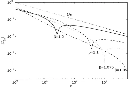
It is also worth looking at the asymptotic behavior ofC2n in the cases whereβ >1.

Figure 2.2 shows such behavior for a series of β values approaching 1 from above, compared to the curve n−1_{. It is known that for the series} P∞

n=1n

−s_, _{s >} _{1 will lead}

to convergence. Thus, if |C2n| decays faster than n−1 up to a scaling factor, we will

see below that the series expansion assumes pointwise convergence for ξ ∈ [0,1). For the case where β = 1 as shown in Figure 2.1, it can be computed numerically that

|C2n| ≈D n−1.14 forn large whereD is a constant.

The figure indicates that forβ = 1.2, 1.1,and 1.075,|C2n|decays faster thanDβn−1

for n < Nβ where Dβ and Nβ are constants determined by β. But eventually, |C2n|

(38)

meaning that P∞

0 |C2n| diverges. For β = 1.05, we only compute |C2n| for n ≤ 5000

due to numerical considerations, but the asymptotic analysis above implies that it will ultimately exhibit the same divergent behavior of P∞

0 |C2n|.

100 101 102 103 104

10−6 10−5 10−4 10−3 10−2 10−1 100

n

C_2n

Asymptotic

Figure 2.1: C2n and Its Asymptotic Approximation for x= 0 andβ = 1.

100 101 102 103

10−8

10−6

10−4

10−2

100

n

|C 2n

| β=1.2

β=1.1

β=1.075

β=1.05 1/n

(39)

Consequently, the results (2.54) serves as a sufficient condition for the pointwise convergence of the series reconstruction. For example, when Qn(ξ) =Tn(ξ),

Pe(ξ)−

N−1 P

n=0

CnTn(ξ)

p

1−ξ2 = Z 1 −1 ∞ P n=0

Tn(y)Tn(ξ)

p

1−ξ2 Pe(y)dy

−Z 1

−1

N−1 P

n=0

Tn(y)Tn(ξ)

p

1−ξ2 Pe(y)dy = Z 1 −1 ∞ P

n=N

Tn(y)Tn(ξ)

p

1−ξ2 Pe(y)dy = lim P→∞

N+P

P

n=N

CnwnTn(ξ)

p

1−ξ2 ≤ M ∞ X

n=N

|Cn|

(2.55)

for any ξ∈[0,1) noticing the fact that ∞

P

n=0

Tn(y)Tn(ξ)

√

1−ξ2 =δ(y).

Since we have established the condition for the convergence of P∞

n=0|Cn| in the

formula (2.54), the same condition will imply

N−1 P

n=0

Cn Qn(ξ)

r(ξ) →P(ξ) (2.56)

asN → ∞, for any ξ∈[0,1).

Furthermore, from the relationship (2.34) between the P´eclet number Pe = σ2 κ and

(40)

2.3 Numerical Results of Series Reconstruction

2.3.1 Reconstruction via Extension to

[

−

1 ,

1]

for

T

₀

(

x

) =

e

−x2

First we carried out the reconstruction for the PDF (2.5) using series approximants

Px,t(ξ)≈ N−1

P

n=0

C2nT2n(ξ)

p

1−ξ2 (2.57)

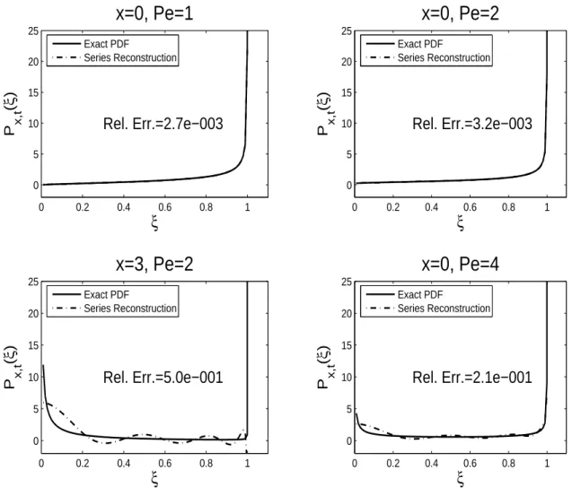
by evenly extending it to [−1,1]. The numerical results are illustrated in Figure 2.3, which compares the exact PDF (solid line) with its series reconstruction (dashed line) obtained by setting N = 4 in (2.57) (first 4 even moments are used). Four reconstruc-tions are done at t = 1 for different x and Pe values. We note that the similar case with an odd extension yields a nearly identical comparison.

The reconstructions in the upper two panels, in which x = 0 and Pe ≤ 2, agree with the exact PDF with error near the singularity ξ = 1, respectively; while the two in the lower panels, in which x 6= 0,Pe = 2 or x = 0,Pe > 2, fail to recover the true distributions almost everywhere. Recall that the series reconstruction is expected to fail wheneverPx,t(0) =∞, since the truncated series (2.57) is always smooth atξ = 0.

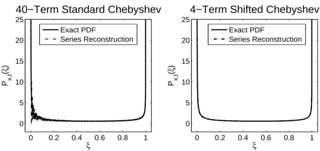
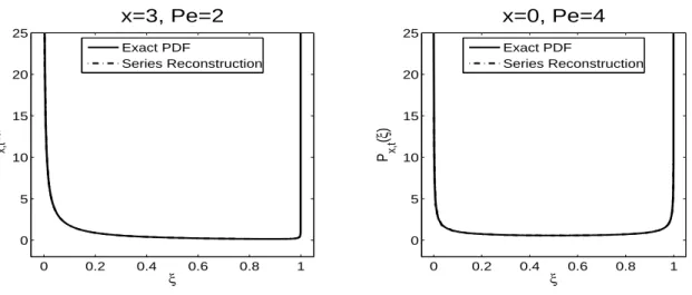
Does an increasingN help reducing the error? The answer is no. In the left panel of Figure 2.4, we increaseN to 40 and compare the series reconstruction using the standard Chebyshev polynomials to the exact PDF for x = 2, t = 1 and Pe = 4. We can see the rapid oscillations nearξ= 0, which is a characteristic of high order polynomials in a finite interval, let alone the fact that to obtain the coefficients about 40 significant digits are required for accurate summation of Eq.(2.42). But an alternative polynomial family can improve the reconstruction. In the right panel, we reconstruct the PDF via shifted Chebyshev polynomials and re-define r(ξ) = pξ3₍₁−_ξ_{). Now only 4 terms}

are needed to approximatePx,t(ξ) with negligible error. We will discuss how and why

alternative choices of r(ξ) and the polynomial family improve the reconstruction later in this section.

(41)

0 0.2 0.4 0.6 0.8 1 0 5 10 15 20 25 ξ P x,t ( ξ )

x=0, Pe=1

Rel. Err.=2.7e−003 Exact PDF Series Reconstruction

0 0.2 0.4 0.6 0.8 1

0 5 10 15 20 25 ξ P x,t ( ξ )

x=0, Pe=2

0 0.2 0.4 0.6 0.8 1

0 5 10 15 20 25 ξ P x,t ( ξ )

x=3, Pe=2

0 0.2 0.4 0.6 0.8 1

0 5 10 15 20 25 ξ P x,t ( ξ )

x=0, Pe=4

Figure 2.3: 4-Term Chebyshev Reconstructions of the PDF at t= 1

is defined by

εN =

kPx,t(ξ)−

PN−1

n=0 C2nT2n(ξ) p

1−ξ2 k2 kPx,t(ξ)k2

. (2.58)

2.3.2 Improving Series Reconstruction

Let us see how alternative choices of r(ξ) and the polynomial family improve the re-construction. Letting r(ξ) = pξ3₍₁−_ξ_{) and} _Q

n(ξ) = Tn∗(ξ) as discussed in Section

(42)

0 0.2 0.4 0.6 0.8 1 0

5 10 15 20 25

ξ

P x,t

(

ξ

)

40−Term Standard Chebyshev

0 0.2 0.4 0.6 0.8 1

0 5 10 15 20 25

ξ

P x,t

(

ξ

)

4−Term Shifted Chebyshev

Exact PDF

Series Reconstruction

Exact PDF

Figure 2.4: Reconstructions of the PDF att = 1 via Different Orthogonal Polynomials

the series reconstruction relies on the capability of (r(ξ))−1 to recover the singularities in Px,t(ξ), since the numerator in (2.57) is always continuous in [0,1]. For example,

when x6= 0 and β ≥1, we know from (2.5) and Table 2.1 that Px,t(0) =Px,t(1) =∞.

Therefore [r(ξ)]−1 _{= [}_ξp

(1−ξ2_)]−1_{, which has two singularities at}_ξ _{= 0 and 1, should}

be adopted instead of [r(ξ)]−1 _{= [}p

(1−ξ2_)]−1_{. Of course,} _r₍_ξ_{) should be defined in}

such a way that r(ξ)w(ξ) =ξk _where _k _{is an non-negative integer and thus the}

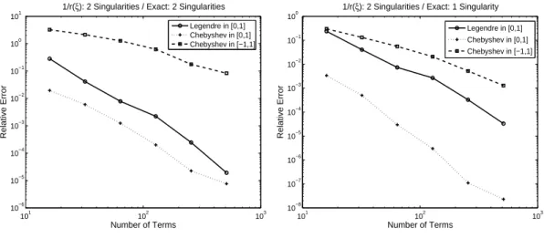
coeffi-cients can be computed using statistical moments as shown in (2.46). Figure 2.7 is a comparison between the convergence rates of reconstructing the same PDF using the following three different combinations ofr(ξ) andQn, each of which corresponds to one

curve in either panel

1. Shifted Legendre polynomials defined on [0,1] and r(ξ) = ξ(1−ξ); 2. Shifted Chebyshev polynomials defined on [0,1] and r(ξ) = pξ3₍₁−_ξ_);

3. Standard Chebyshev polynomials defined on [−1,1] and r(ξ) = ξp1−ξ2_.

In the left panel of Figure 2.7, x = 3, Pe = 2 and t = 1, so Px,t(0) = Px,t(1) =∞;

whereas on the right,x= 0, Pe = 2 andt= 1, soPx,t(0) = 0, Px,t(1) =∞. Notice that

the number of singularities in [r(ξ)]−1_{is greater than (right) or equal to (left) that of the}

(43)

100 300 500 700 900 1000 10−6

10−5 10−4 10−3 10−2 10−1 100 101

Number of Terms

Relative Error

x=0,t=1,β=0.5

x=0,t=1,β=1

x=3,t=1,β=1

x=0,t=1,β=4

Figure 2.5: Relative Errors of Series Reconstructions VS Number of Terms Kept in (2.57)

0 0.2 0.4 0.6 0.8 1

0 5 10 15 20 25

ξ P x,t

(

ξ

)

x=3, Pe=2

0 0.2 0.4 0.6 0.8 1

0 5 10 15 20 25

ξ P x,t

(

ξ

)

x=0, Pe=4

Exact PDF

Series Reconstruction Exact PDF

Figure 2.6: 4-Term Shifted Chebyshev Reconstructions of the PDF at t= 1

for some ξ∗ ∈[0,1] when this occurs.

(44)

101 102 103 10−6

10−5 10−4 10−3 10−2 10−1 100 101

Number of Terms

Relative Error

1/r(ξ): 2 Singularities / Exact: 2 Singularities

Legendre in [0,1] Chebyshev in [0,1] Chebyshev in [−1,1]

101 102 103

10−8 10−7 10−6 10−5 10−4 10−3 10−2 10−1 100

Number of Terms

Relative Error

1/r(ξ): 2 Singularities / Exact: 1 Singularity

Legendre in [0,1] Chebyshev in [0,1] Chebyshev in [−1,1]

Figure 2.7: Convergence Rates for Different r(ξ) andQn(ξ)

2.4 Monte-Carlo Simulations and PDF Dynamics

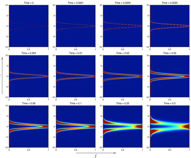
The purpose of this section is to study the effectiveness of Monte-Carlo methods ap-plied in the problem (3.1), when the exact PDF for the tracer is known at all times. The Monte-Carlo simulation for Eq.(3.1) is straightforward by spectral methods, along with a simple random number generator. Moreover, at a fixed timet, the Monte-Carlo simulation for the tracer can be made easier by samplingW(t) from a mean-zero Gaus-sian random variable with variance σ2tfrom the scaling property of Wiener Processes. Nonetheless, to study the full temporal evolution of Px,t(ξ), one has to simulate the

complete Wiener pathW(t), which is discretized as a sum of independent Gaussian ran-dom variables using standard techniques(Gardiner, 1985), namely, W(t) ' PN

i=0dwi

wheredwi ∼ N(0, σ2∆ti).

For general stochastic flows and initial data, the analytic solution to the random advection-diffusion problem is not available as well as the exact scalar PDF. Monte-Carlo simulation is a powerful numerical tool to approximate the PDF and investigate its dynamics in such cases. Moreover, accurate Monte-Carlo simulations can be used to benchmark the performance of the PDF reconstructions via orthogonal polynomials discussed in the previous sections.

2.4.1 Uni-Modal Positive, Gaussian Initial Data

T

₀

(

x

) =

e

−x2

We will first examine the case with the initial dataT0(x) =e−x

2

(45)

and recover its spatio-temporal dynamics with a certain number of realizations.

Monte-Carlo Simulations

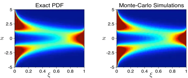
Figure 2.8 depicts the spatial structure ofPx,t(ξ) obtained by two different approaches:

exact formula (2.5) and Monte-Carlo simulations. Here Pe = 2 and t = 1. To obtain each histogram to simulatePx,t=1(ξ), 105 samples are drawn by the Monte-Carlo

simu-lator and 100 bins are distributed uniformly between [0,1]. Each panel is a snapshot of

Px,t(ξ), exact on the left and Monte-Carlo simulated on the right, at time t = 1. The

horizontal axis is the renormalized scalar ξ-axis, ranging from 0 to 1, and the vertical axis is the spatial x-axis between [−5,5]. The grayscale ramp is set uniformly between [0,2] such that regions wherePx,t(ξ)≈0 are dark blue, whereas dark red regions implies

Px,t(ξ)&2. For example, if we take a horizontal slice of the left panel alongx= 3, and

interpret the brightness with corresponding numbers, we would recover the solid curve shown in the lower-left panel of Figure 2.3.

ξ

x

ξ

x

Figure 2.8: Comparison Between the Exact PDF (2.5) and MC Simulations. Horizon-tal Axis — Renormalized Tracer ξ. Vertical Axis — Spatial Variable x. *: Grayscale ramp uniformly set in [0,2], same in all other grayscale figures

(46)

panel is defined similarly to Eq.(2.58) by replacing the series reconstruction with the simulated histogram.

100 101 102 103 104

10−2 10−1 100

n

<

ξ

n>

107 Realizations

Simulated Moments Exact Moments

104 105 106 107

10−2 10−1

Number of Realizations

Relative Error

Figure 2.9: Benchmarking the Monte-Carlo Simulator. Left: Exact Moments VS Simulated Moments. Right: Relative Error in Px,t(ξ) VS Number of Realizations.

In the left panel, we can see that the simulated moments coincide with the exact moments for n _. 1000. The right panel depicts the L2 relative error which shows improved convergence with the number of realizations increasing from 104 to 107. With increasing M, the number of realizations, the relative error first decays like √1

M, while

it remains almost the same forM ≥106_{. We also find that the pointwise relative error}

is negligible (∼ 0.1%) when M ≥ 105 _{everywhere in [0}_,_{1] except near the singularity}

ξ= 1. This error saturation is however inevitable with any simulation approach because of the systematic bias introduced by discretization errors, the finite statistics, histogram binning, etc.

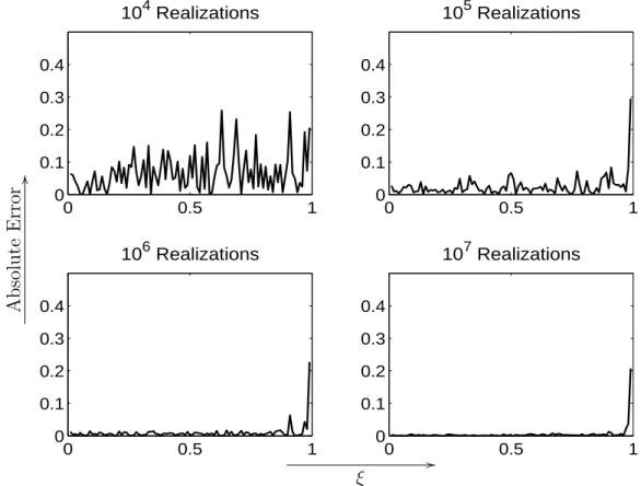
We next explore the decay of the pointwise, absolute error of the Monte-Carlo simu-lation with increasing number of realizations. Figure 2.10 shows the difference between

P0,10(ξ) and its Monte-Carlo approximations. And we can see that with increasing

number of realizations, the pointwise error vanishes except near ξ = 1, which is the singularity inP0,10(ξ). This is however inevitable with any Monte-Carlo approach since

Passive scalar intermittency in random flows