Bank Market Power and Central Bank Digital
Currency: Theory and Quantitative Assessment
∗
Jonathan Chiu
†Bank of Canada
Mohammad Davoodalhosseini
‡Bank of Canada
Janet Jiang
§Bank of Canada
Yu Zhu
¶Bank of Canada
June 30, 2020
Abstract
This paper develops a micro-founded general equilibrium model of payments to study the impact of a central bank digital currency (CBDC) on intermediation of private banks. If banks have market power in the deposit market, a CBDC can enhance com-petition, raising the deposit rate, expanding intermediation, and increasing output. A calibration to the U.S. economy suggests that a CBDC can raise bank lending by 1.53% and output by 0.11%. We evaluate various design features of the CBDC, including its interest, acceptability, eligibility as reserves and the supply rule. We also assess the role of a CBDC as the use of cash declines.
JEL Codes: E50, E58.
Keywords: Central bank digital currency; Banking; Market power; Monetary policy; Disintermediation
∗This paper was circulated under the title “Central Bank Digital Currency and Banking.” We are grateful to Todd Keister for his insightful comments throughout the project. We thank Rod Garratt, Charlie Kahn, Peter Norman, Eric Smith, Randall Wright and our Bank of Canada colleagues for their comments and suggestions. We also thank participants of the following conferences for their comments: Conference on the Economics of CBDC by Bank of Canada and Riksbank, Conference of the European Association for Research in Industrial Economics, IMF Annual Macro-Financial Research Conference, the Society for the Advancement of Economic Theory, Annual Meeting of the Society for Economic Dynamics, Midwest Macroeconomic Meeting and SNB-CIF Conference on Cryptoassets and Financial Innovation. The views expressed in this paper are those of the authors and not necessarily the views of the Bank of Canada.
1
Introduction
Central banks in several countries, including China, Canada and Sweden, are considering
issuing central bank digital currencies (CBDCs), a digital form of central bank money that
can be used for retail payments. One frequently raised concern about a CBDC is that, since it
is likely to compete with bank deposits as a payment instrument, it may increase commercial
banks’ funding costs and reduce bank deposits and loans, leading to bank disintermediation.1
For example, the International Monetary Fund (IMF) staff discussion note by Mancini-Griffoli et al. (2018) argues that “as some depositors leave banks in favor of CBDC, banks
could increase deposit interest rates to make them more attractive. The higher deposit rates
would reduce banks’ interest margins. As a result, banks would attempt to increase lending
rates, though at the cost of loan demand.” The 2018 report by the Committee on Payments
and Market Infrastructures of the Bank for International Settlement raises the same concern.
This study aims to formally assess this concern,both theoretically and quantitatively. We first develop a general equilibrium model of payments and bank intermediation. In the model,
households allocate funds between two assets or payment instruments, cash and checkable
deposits, that differ in terms of the types of exchange they can facilitate. For example, cash cannot be used in online transactions while deposits can be used via debit/credit cards or
electronic transfers. Entrepreneurs have investment opportunities but no resources.
House-holds can produce the investment good and need deposits as a means of payment. Banks act
as intermediaries, creating deposits and issuing loans to entrepreneurs subject to a reserve
requirement. One critical feature of our model is the imperfect competition in the deposit
market, which is consistent with the empirical findings in Dreschler et al. (2017) and Wang
et al. (2018).
To highlight the main mechanism of this paper, we first introduce a baseline CBDC into
the model. This CBDC is a perfect substitute for bank deposits as a means of payment, bears interest and cannot be held by banks. We examine how the interest rate on the CBDC
affects deposits, loans, and the total output. We then allow banks to hold the CBDC as
reserves. Finally, we study the role of a non-interest-bearing CBDC when the use of cash in
the economy continues to decline. We consider this scenario because it is of particular policy
interest. It has been experienced by several countries and is cited as an important reason
for issuing a CBDC. The COVID-19 pandemic may further accelerate this trend.2 We also
discuss other design choices in terms of acceptability and the rule of supply (for example,
fixed quantity or rate).
Our model predicts that if banks have market power in the deposit market, the impact of
a CBDC is non-monotone in its interest rate. It expands bank intermediation if its rate is intermediate and causes disintermediation if its rate is too high. This finding is robust to how
we model the deposit market and the loan market. In the main text, we focus on Cournot quanity competition in the deposit market and perfect competition in the loan market. In
the Appendix, we allow for an imperfectly competitive loan market, and also study a model
with price competition in the deposit market following Burdett and Judd (1983) and Head
et. al (2012).3
The main mechanism through which a CBDC “crowds in” bank intermediation works as
follows. In an imperfectly competitive deposit market, banks restrain deposit supply to keep
interest rates on deposits lower than (or equivalently, the price of deposits higher than) the
level under perfect competition. A CBDC offers an outside option to depositors and sets an
interest rate floor for bank deposits.4 This interest floor reduces commerical banks’ incentive to restrain deposit supply because it limits the reduction in the deposit rate. As a result
commerical banks supply more deposits, lower the loan rate and expand lending when the
reserve requirement is binding.
Interestingly, the CBDC may or may not be used in the equilibrium depending on its interest
rate. However, it can have a positive effect on deposits, loans and output even if it has
zero market share. The existence of a CBDC as an outside option forces banks to match the CBDC rate, and create more deposits and loans.5 This is different from the standard
2For example, see the Payment Canada report “COVID-19 pandemic dramatically shifts Canadians’ spending habits.”
3We thank Eric Smith for suggesting this version of the model.
4This suggests that the CBDC rate could have stronger pass-through to deposit rate than traditional monetary policy tools, which do not seem to affect deposit rates much. For example, the policy rate in the U.S. increased by 2% from 2016 to 2018, but commercial banks barely moved their deposit rates, measured as the national rate on non-jumbo deposits (less than $100,000) for money market, savings, or interest checking accounts (source: FDIC, Money Market [MMNRNJ], Savings [SAVNRNJ] and Interest Checking [ICNRNJ] data series retrieved from FRED, April 15, 2020). On a related note, Berentsen and Schar (2018) argue that a CBDC would make monetary policies more transparent as the interest rate on a (publicly accessible) CBDC would set a floor for the deposit rate.
competition effect where total quantity increases as a result of more suppliers. The suppliers
of deposits and loans remain unchanged and the CBDC can induce them to supply more. A
policy implication is that one should assess the effectiveness of a CBDC based on its effect
on deposits or the deposit rate instead of its usage.
Calibrating our model to the U.S. economy, we find that the baseline CBDC expands bank
intermediation if the interest rate on the CBDC is between 0.30% and 1.28%. At the
maxi-mum, a CBDC can increase loans and deposits by about 1.53% and the total output by about
0.11%. The positive effect reverses if the CBDC rate exceeds 1.28%. To stay break-even,
banks are forced to raise the lending rate to compensate for the interest paid on deposits, which reduces loans and deposits.6 If the CBDC serves as reserves, it promotes bank
inter-mediation for a wider range of interest rates and its effect is also slightly stronger. Finally,
even if a CBDC bears zero interest, it can restrict banks’ market power and improve
inter-mediation as the economy becomes increasingly cashless, i.e., use of cash declines. Without
a CBDC, banks could reduce intermediation and pay negative deposit rates.
Our study is closely related to two concurrent papers. Keister and Sanches (2019) focus on
the welfare implication of an interest-bearing CBDC when the banking sector (modelled as a
bank-firm combination) is perfectly competitive. Banks are subject to financial frictions
be-cause of the limited pledgeability of their projects. Keister and Sanches (2019) highlight the trade-off that the CBDC always crowds out bank intermediation, but can promote efficiency
in exchange. The benefit of efficient exchange dominates the cost from disintermediation if
financial frictions are not very severe.
Andolfatto (2018) studies the effect of a CBDC on bank intermediation in an economy with
heterogeneous households and a monopolistic bank. He uses the overlapping generations
framework where young households save for old age in cash, deposits or a CBDC. The latter
two require costly access to the banking system, so poor households save only in cash. He
shows that a CBDC could compel the bank to increase the deposit rate, which increases financial inclusion and bank deposits. On the lending side, he assumes that the central bank
lends unlimitedly to the commercial bank at a fixed rate, which fully determines the level of
loans and disconnects the bank’s loans from its deposits.
used in equilibrium.
Compared to these two papers, our framework is more suitable for quantifying the effect of
a CBDC and accommodates various design choices as the payment landscape evolves. First,
our model captures a full spectrum of competitiveness. If the number of banks is one, the
banking sector is monopolistic as in Andolfatto (2018). If this number tends to infinity,
the banking sector is perfectly competitive as in Keister and Sanches (2019). We use data
to discipline the level of competitiveness, which is crucial for quantifying the impact of a
CBDC. Second, we explicitly model cash, deposits and a CBDC as different but imperfectly
substitutable payment instruments to facilitate different types of transactions. This allows
us to discuss the design of the CBDC in terms of its acceptability and its effect when the
payment landscape evolves, e.g., the use of cash declines. Finally, modelling the reserve requirement allows us to discuss another issue regarding the design of a CBDC: whether it
can be held as bank reserves.
This paper focuses on the effects of a CBDC on competition and abstracts from issues such
as banks’ risk taking behavior and financial stability. For work on these aspects, see Monnet
et. al (2019), Chiu et. al (2019) and Fern´andez-Villaverde et al. (2020a,b).
There are a number of papers that study other implications of a CBDC. Barrdear and
Kumhof (2016) develop a DSGE model and estimate that issuing a CBDC could increase
GDP by up to 3% mostly through reducing real interest rates. Brunnermeier and Niepelt (2019) derive conditions under which the issuance of inside money and outside money are
equivalent, even if inside money and outside money have liquidity or return differences. Their
results imply that introducing a CBDC does not necessarily change macroeconomic
out-comes. Davoodalhosseini (2018) studies a model where a CBDC allows balance-contingent
transfers, but is more costly to use than cash. He finds that the co-existence of cash and
the CBDC may not be optimal, because cash can serve as an outside option for agents,
re-stricting the central bank’s power in implementing balance-contingent transfers. Williamson
(2019) argues that a CBDC can raise issues regarding independence of the central bank and
scarcity of assets eligible to back the CBDC. Dong and Xiao (2019) show that certain types of CBDC can be useful in implementing a negative policy rate.7
Our paper is related to the literature on transmission channels of monetary policy through
the banking system. In their seminal work, Bernanke and Blinder (1992) propose a bank
reserve channel. A higher interest rate increases the opportunity cost of holding reserves,
leading banks to reduce their lending. This channel also operates in our model. Dreschler,
Savov, and Schnabl (2017) propose a transmission channel based on banks’ market power
in deposit markets. A higher nominal interest rate makes cash more expensive relative to
deposits, and banks with market power raise the spread between the nominal interest rate
and the deposit rate. The mechanism through which a higher interest on a CBDC raises
the deposit rate and quantity in our model is similar to the mechanism through which an
expansionary policy works in their paper: both policies reduce the banks’ market power in the
deposit market. Different from their paper, we model lending and the payment arrangements
explicitly. These features allow us to study the macroeconomic effects on production and consumption, and to conduct various counterfactual analyses regarding the effects of CBDCs
with different design choices.8
Finally, our paper contributes to the New Monetarist literature with financial intermediation
by modeling imperfect competition in inside money creation. Berentsen, Camera, and Waller
(2008) first incorporate banking into the Lagos and Wright (2005) model. Their banking
sector is perfectly competitive and does not create inside money. Gu et al. (2018) show that
banking sector is inherently unstable. Consistent with their findings, our banking sector is
potentially unstable because it may lead to multiple equilibria; see AppendixB. Dong et al. (2016) study a model of oligopolistic banks that face mismatch in the timing of payments,
and show that both bank profits and welfare are non-monotone in the number of banks.
This paper is organized as follows. Section2introduces the baseline model, where there is no CBDC. Section3derives the equilibrium of the baseline model. Section4studies the impact of a CBDC that cannot be held by banks to illustrate the main mechanism of this paper.
Section 5 analyzes the case where banks can hold CBDC as reserves. Section 6 calibrates the model and assesses the quantitative implications. Section 7 discusses the robustness of our results in different extensions of the model. It also discusses two alternative designs of a
CBDC. Section 8concludes. The omitted proofs and calculations are collected in Appendix
A. Extensions and further discussions come in other appendices.
2
Environment
Time is discrete and continues forever from 0 to infinity. There are four types of agents: a
continuum of households with measure 2, a continuum of entrepreneurs with measure 1, a
finite number of N bankers, and the government. The discount factor from current to the
next period is 0 < β < 1. In each period t, agents interact sequentially in two stages: a
frictionless centralized market (CM), and a frictional decentralized market (DM). There are
two perishable goods: good x in the CM and good y in the DM.
Households are divided into two permanent types, buyers and sellers, each with measure 1.
In the CM, both types work and consumex. Their laborhis transformed intoxone-for-one.
In the DM, buyers and sellers meet bilaterally and trade good y. Buyers want to consume
y, which can be produced on the spot by the sellers. The utility from consumption is u(y)
with u0 >0, u0(0) =∞, and u00 <0. The disutility from production is normalized to y. Let
y∗ be the socially efficient DM consumption, which solvesu0(y∗) = 1. To summarize, buyers
and sellers have period utilities given respectively by
UB(x, y, h) = U(x)−h+u(y),
US(x, y, h) = U(x)−h−y.
Young entrepreneurs are born in the CM and become old and die in the next CM.
En-terpreneurs cannot work in the CM and care about only consumption when old. Young
enterpreneurs are endowed with an investment opportunity that transforms x current CM
goods to f(x) CM goods in the next period, where f0(0) = ∞, f0(∞) = 0, f0 > 0, and
f00<0.
Given the preferences and endowment, there are gains from trade between buyers and
sell-ers, and between entrepreneurs and households. Buyers would like to consume DM goods
produced by sellers, and entrepreneurs would like to borrow from houeholds to invest in their investment opportunities. However, entrepreneurs lack commitment and households cannot
enforce debt repayment, so credit arrangement among them is not viable.
Like entrepreneurs, young bankers are born in the CM and will become old and die in the
next CM.9 They cannot work in the CM and consume only when old. Unlike households
and entrepreneurs, bankers can commit to repay and enforce payment (refer to Gu et al.,
2018, for the discussion of the endogenous emergence of banks). Each of the bankers runs a
bank. As a result, banks can act as intermediaries between households and entrepreneurs to
finance the investment projects. A bank has the option to issue illiquid or liquid deposits.
Illiquid (time) deposits cannot be used to make payments, while liquid (checkable) deposits
can.
The government issues fiat money, which is a physical token and can be used as a means
of payment. Throughout the paper, we use “fiat money” and “cash” interchangeably. The
supply of fiat money Mt grows at a constant gross rate µ > β. The change in the supply
is implemented through lump-sum transfers to (if µ > 1) or taxes on (if µ <1) households. The government also stipulates a reserve requirement that a bank’s cash holding must cover
at least χfraction of its checkable deposits.
As in Zhu and Hendry (2019), there are three types of meetings in the DM, depending on
which of the two means of payment, cash and deposits, can be used for transactions. From
a buyer’s perspective, with α1 >0 probability, a buyer enters into a type 1 meeting, where
only fiat money can be used. With α2 >0 probability, a buyer enters into a type 2 meeting,
where only bank deposits can be used. Withα3 ≥0 probability, a buyer enters into a type 3
meeting, where both can be used. The three types of meetings can be interpreted as follows.
Type 1 meetings are transactions in local stores that do not have access to debit cards; type 2 meetings are online transactions where the buyers and sellers are spatially separated and
can only use debit cards or bank transfers; and type 3 meetings occur at local stores with
point-of-sale (POS) machines, and hence both payment methods are accepted.
Agents in our model engage in the following activities. In every CM, young bankers issue
deposits for two purposes. First, banks issue deposits to households in exchange for fiat
money which can be kept as bank reserves. Second, banks offer loans to entrepreneurs in
the form of deposits, which entrepreneurs use to buy x from households for investment.
In the DM, buyers use a combination of cash and checkable deposits to purchase goods y from sellers. In the following CM, deposits and loans are settled. Entrepreneurs sell some
of the investment output for cash or deposits to settle bank loans and retain the remaining
output for their own consumption. Having collected the loan repayments, bankers redeem the
deposits held by the households and retain the remaining profit for their own consumption.
Figure1 presents the timeline for all agents.
For the analysis in the main text, we assume that banks engage in Cournot competition in the
deposit market, but the lending market is perfectly competitive. We choose to focus on this
(a) Buyers
(b) Sellers
(c) Entrepreneurs
(d) Bankers
than in the loan market (Dreschler et al., 2017; Wang et al., 2018). In Appendix C, we extend the model to the case where the lending market also features imperfect competition.
3
Equilibrium without a CBDC
In this paper, we focus on the steady-state monetary equilibrium, where cash has positive
value. It takes four steps to solve for the equilibrium. First, we characterize the household’s
problem to derive the demand for cash and bank deposits. Second, we lay out the problem
faced by the bank, incorporating the household demand for deposits, to derive the aggregate supply for loans. Third, we derive the aggregate demand for loans. Finally, we equate the
supply and demand for loans to derive the market clearing loan rate, and combine it with
the solutions to all agents’ problems to characterize the equilibrium deposit rate, real cash
balances (held by households and banks as reserves), and the quantities of deposits and
loans.
3.1
Households
We first examine the buyer’s maximization problem, and then the seller’s problem. Let W
andV be the value functions of households in the CM and DM, respectively. In the following,
we suppress the time subscript and use prime to denote variables in the next period.
In the CM, a buyer chooses consumption x, laborh, and the real cash, checkable and time deposit balances in the next period, z0, d0 and b0.10 The buyer’s value function is
WB(z, d, b) = max
x,h,z0,d0,b0
U(x)−h+βVB(z0, d0, b0)
st. x = h+z+d+b+T − φ
φ0z 0 −
ψd0−ψbb0,
where φ is the price of cash in terms of CM good, and ψ and ψb are the prices of future
real checkable and time deposit balances, respectively. The real return on cash balances is φ0/φ−1, the real interest rate on checkable deposits is 1/ψ−1, and the real interest rate
on time deposits is 1/ψb −1. Substitute out h using the budget equation and rewrite the
buyer’s CM problem as
WB(z, d, b) = z+d+b+T + max
x [U(x)−x]
+ max
z0,d0,b0
−φ
φ0z 0−
ψd0−ψbb0+βVB(z0, d0, b0)
.
Note thatWB(z, d, b) is linear inz, d, and b. The first-order conditions (FOCs) are
x : U0(x) = 1,
z0 : φ φ0 ≥βV
B
1 (z 0
, d0, b0), with equality ifz0 >0,
d0 : ψ ≥βV2B(z0, d0, b0), with equality if d0 >0,
b0 : ψb ≥βV3B(z 0
, d0, b0), with equality if b0 >0,
where the subscripts indicate the derivative with respect to corresponding arguments. Two
standard results are that all buyers choose the same portfolio (z0, d0, b0), and WB(z, d, b) is linear in (z, d, b) with WB
1 (z, d, b) = W2B(z, d, b) =W3B(z, d, b) = 1.
The buyer’s DM value function is
VB(z, d, b) = α1[u◦Y (z)−P (z)] +α2[u◦Y (d)−P (d)] (1)
+α3[u◦Y (z+d)−P(z+d)] +WB(z, d, b) ,
where Y (·) and P (·) are the terms of trade (TOT) and represent the amount of good y
being traded and the amount of payment, respectively. The TOT depends on the buyer’s
usable liquidity, which varies according to the type of meetings. We will discuss the TOT in
detail later.
Now we characterize the seller’s problem. The seller enters the DM with zero liquidity
balances, or z0 =d0 = 0, because he/she does not need liqiuid in the DM. Using this result,
we can formulate the seller’s CM problem as
WS(z, d, b) = max
x,h
U(x)−h+βVS(0,0, b0)
st. x+ψbb0 = h+z+d+b+T.
value function is
VS(0,0, b) = α1[P (˜z)−Y (˜z)] +α2 h
P
˜ d
−Y
˜ d
i
+α3 h
P z˜+ ˜d−Y z˜+ ˜di+WS(0,0, b),
where ˜d and ˜z are the cash and deposit holdings of his/her trading partner.
The TOT are determined by buyers making take-it-or-leave-it offers. Let L be the buyer’s
total available liquidity, which is equal to z in type 1 meetings, d in type 2 meetings, and
d+z in type 3 meetings. The buyer offers an output-payment pair (y, p) to solve
max
y,p [u(y)−p] s.t. p≥y and p≤ L,
where the first constraint is the seller’s participation constraint and the second the liquidity
constraint. The TOT as a function of the buyer’s total available liquidity L are
Y (L) =P (L) = min(y∗,L). (2)
In words, if the buyer has enough payment balances to purchase the optimal amount, then
the optimal amount is traded; otherwise, the buyer spends all available payment balances.
Combining the FOCs of buyers with respect to z0 and d0 in the CM and equations (1) and (2), we obtain the buyer’s demand for payment balances,
φ
βφ0 = α1λ(z 0
) +α3λ(z0+d0) + 1,
ψ
β = α2λ(d
0
) +α3λ(z0+d0) + 1,
where λ(L) = max [u0(L)−1,0] is the liquidity premium. Note that the demand for cash
and deposits is positive if u0(0) = ∞, α1 > 0 and α2 >0. At the steady state, z and d are
constant over time. Then φ/φ0 =µ and the demand for liquid balances (z, d) is given by
ι = α1λ(z) +α3λ(z+d), (3) ψ
β −1 = α2λ(d) +α3λ(z+d), (4)
where ι = µ/β − 1 is the nominal interest rate using the Fisher’s equation. These two
the fact that the buyer can use the marginal unit of cash in type 1 and type 3 meetings to
derive λ(z) and λ(z+d) additional units of utility, respectively, from consumption. The
second equation is for checkable deposits and has a similar interpretation.
Here, (3) defines the aggregate demand for cash balancesz as a function ofd. Given this, (4) defines the aggregate inverse demand function for checkable deposits, ψ = Ψ(d). It has the
following properties: Ψ(0) = ∞, Ψ(d) = β for d ≥ y∗, Ψ0(d)< 0 for d < y∗, and Ψ0(d) = 0
for d≥y∗.11
Finally, the demand for time deposits is separate from the demand for liquid assets and is
given by
ψb = β.
In words, since time deposits have no liquidity value, their return must compensate for
discounting across time.
3.2
Banks
Banks issue two types of deposits, checkable deposits (d) and time deposits (b), to
house-holds, and invest in two assets, cash (z) and loans (`).12 The N bankers engage in Cournot competition in the deposit market and perfect competition in the loan market. Bankers face
a reserve requirement.13 At the end of each CM, the real value of a banker’s cash holding
must be at least χfraction of the total checkable deposits, whereχ is a policy parameter set
by the government.
Formally, banker j solves the following maximization problem, taking the price of time
deposits (ψb = β), the market loan rate (ρ) and other banks’ checkable deposit quantities
11From (3) and (4), Ψ0(d) =α
2βλ0(d) +
α1α3βλ0(z+d)λ0(z)
α1λ0(z)+α3λ0(z+d)≤0, with strict inequality ifd < y
∗.
12In most cases, the time deposit is not issued in the equilibrium. However, it eliminates some uninteresting technical issues. Our main results remain unchanged if we remove it.
(D−j =Pi6=jdi) as given:
14
max
zj,`j,dj,bj
(1 +ρ)`j +
zj
µ −dj−bj
(5)
s.t. `j +zj = Ψ (D−j+dj)dj+βbj,
zj ≥χΨ (D−j+dj)dj.
The banker maximizes consumption in the second period of life. He/She receives the
re-payment of loans (principal plus interest) from the entrepreneurs, (1 +ρ)`j, the
inflation-adjusted value of money holdings, and redeems the deposits dj and bj. Here zj is real cash
balances in the banker’s first CM. These cash balances are worth φ0zj/φ =zj/µ in the
sec-ond CM because of inflation. And dj and bj are the after-interest values of deposits in the
banker’s second CM. The before-interest values of deposits are Ψ(D−j+dj)dj andβbj, which
capture the amount of resource bankerj has in his first CM. The maximization problem has
two constraints. The first constraint is the balance sheet identity of the bank at the end of
the banker’s first CM. The right-hand side is the liability, which includes the before-interest
real value of checkable and time deposits. The left-hand side is the asset, which includes
cash and loans. The second constraint reflects the reserve requirement. We also implicitly
impose that dj, bj,zj, `j are non-negative throughout the paper.
In the following, we analyze the Cournot competition in the deposit market given the loan
rate ρ. We focus on the symmetric equilibrium where every bank makes the same choice.
Note that if 1 +ρ >1/β, then the bank can make unlimited profits by issuing time deposits and investing in loans. As a result, 1 +ρ ≤ 1/β in equilibrium. There are four cases
depending on the magnitude of 1 +ρ relative to the gross return on cash, 1/µ, and the gross
return on time deposits, 1/β.
Case 1: cash has a higher return than loans. If 1 +ρ < 1/µ, then the bank does not
invest in loans (`= 0) because its return is dominated by cash. The bank’s asset consists of
only cash, and the reserve requirement does not bind. The bank’s problem can be rewritten
as
max
zj,dj,bj
zj
µ −dj −bj
s.t. zj = Ψ(D−j +dj)dj +βbj.
14Note that banks cannot affect the price of time deposits, which is fixed atψ
b=β from the household’s
Use the balance sheet identity to eliminate zj and obtain
max
dj,bj
Ψ(D−j +dj)dj+βbj
µ −dj−bj
The first-order condition for dj is
dj : Ψ0(D−j +dj)dj + Ψ(D−j +dj) = µ.
The derivative with respect to bj is β/µ−1 < 0, implying bj = 0; i.e., the bank does not
issue time deposits because the return on cash is less than the deposit rate required by the
household, 1/β. In a symmetric equilibrium, each bank issues dµ units of checkable deposits
and invests only in cash (zj = Ψ(N dµ)dµ), where dµ solves
Ψ0(N dµ)dµ+ Ψ(N dµ) = µ.
Case 2: cash and loans have the same return. If 1 +ρ = 1/µ, then the bank is
indifferent between investing in loans and cash reserves as long as the reserve requirement is satisfied. The supply of (checkable and time) deposits remains the same as in case 1. The
supply of loans for each bank lies in the interval [0,(1−χ)Ψ(N dµ)dµ].
Case 3: loans have a higher return than cash. If 1 +ρ > 1/µ, then the reserve
requirement binds, and we can rewrite the bank’s problem using the constraints to eliminate
`j and zj in the objective function in (5) as
max
dj,bj
(1 +ρ)[(1−χ)Ψ(d−j +dj)dj +βbj] +
χΨ(d−j +dj)d
µ −dj−bj
.
The first-order condition for dj is
dj : Ψ0(d−j+dj)dj+ Ψ(d−j +dj) =
1
(1 +ρ)(1−χ) +χ/µ.
In a symmetric equilibrium, the supply of checkable deposits for each bank, d, solves
Ψ0(N d)d+ Ψ(N d) = 1
(1 +ρ)(1−χ) +χ/µ, (6)
where the denominator is the gross rate of return on the bank’s assets, which is a weighted
bj is (1 +ρ)β−1. We can further divide case 3 into two sub-cases depending on the relative
magnitudes of 1 +ρ and β.
Case 3a. If 1/µ < 1 +ρ < 1/β, then banks will not issue time deposits because the
required return on time deposits exceeds the return on loans. The bank splits its checkable
deposits between cash reserves in the amount of z =χΨ(N d)d and loans in the amount of
`= (1−χ)Ψ(N d)d.
Case 3b. If 1 +ρ = 1/β, then banks may issue time deposits. The amount of checkable
deposits is given by dβ, which solves equation (6) at ρ= 1/β−1:
Ψ0(N dβ)dβ + Ψ(N dβ) =
1
(1−χ)/β+χ/µ.
The amount of cash reserves is zβ = χΨ(N dβ)dβ. A bank’s loan supply is `β = [(1 −
χ)Ψ(N dβ)dβ,∞). To finance the loans, the bank issues dβ checkable deposits and b =
[`β −(1−χ)Ψ(N dβ)dβ]/β time deposits.
Notice that the loan supply may be indeterminant for certain values ofρ. Therefore, we say
that the Cournot game has a unique symmetric equilibrium if the checkable deposit supply is unique. To establish existence and uniqueness of the equilibrium in the Cournot game,
the following assumption is imposed throughout the paper.
Assumption 1 a) Given any D−j ∈[0, y∗) and κ > β, either there exists a unique dj >0
such that Ψ0(D−j+d)d+ Ψ (D−j +d) ≷ κ if d ≶dj, or Ψ0(D−j +d)d+ Ψ (D−j+d) < κ
for all d≥ 0. b) Ψ0(N d)d+ Ψ (N d) decreases with d on [0, y∗/N) and is larger than µ for sufficiently small d.
Part (a) of this assumption states that Ψ0(D−j+d)d+ Ψ (D−j+d)−κ as a function of d
crosses the horizontal axis from the above and at most once. It guarantees that the best response of banker j to any amount of checkable deposits (less than y∗) created by other
banks is unique. Part (b) plays three roles. First, it ensures the uniqueness of the symmetric
Nash equilibrium in the Cournot game. Second, it implies that the equilibrium checkable
deposits is increasing in ρ. Lastly, it guarantees that banks issue checkable deposits for any
ρ.15
Proposition 1 The Cournot game has a unique symmetric pure strategy equilibrium if
ρ ≤ 1/β −1. In the equilibrium, each bank supplies d(ρ) checkable deposits, where d(ρ) 15Suppose u(y) = y1−σ
1−σ. Assumption 1 holds if ι is sufficiently small and σ < 1. The last part of
Figure 2: Loan Market Equilibrium
is increasing in ρ and solves:
Ψ0(N d)d+ Ψ(N d) = min
µ, 1
(1 +ρ)(1−χ) +χ/µ
. (7)
Proof. See Appendix A.1.
The equilibrium loan supply of an individual bank is
`(ρ) =
0 if 1 +ρ <1/µ,
[0,(1−χ)d(ρ)Ψ(N d(ρ))] if 1 +ρ= 1/µ,
(1−χ)d(ρ)Ψ(N d(ρ)) if 1/µ <1 +ρ <1/β, [(1−χ)dβΨ(N dβ),∞] if 1 +ρ= 1/β.
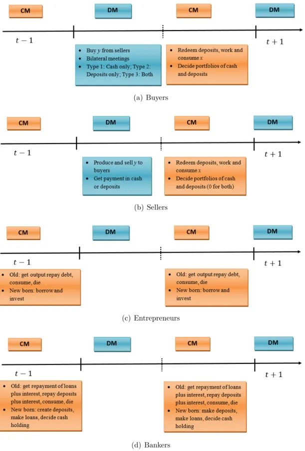
Then we obtain the aggregate loan supply of the banks Ls(ρ) =N `(ρ). It is represented by
the solid black line in Figure2in the (1+ρ)-Lspace. If 1+ρ <1/µ, then banks invest only in cash and the aggregate loan supply is zero. If 1+ρ= 1/µ, then banks are indifferent between lending and holding cash as long as they meet the reserve requirement. The aggregate loan
supply curve is vertical and can take any value between 0 and (1− χ)N dµΨ(N dµ). On
(1/µ,1/β), the aggregate loan supply curve can in principle be non-monotone, which can be
a source for multiple equilibria. However, it is increasing if DΨ(D) is increasing in D, i.e.,
the before-interest value of checkable deposits is increasing in their after-interest value. If
checkable deposits, and if 1 +ρ= 1/β, the supply beyond the amount financed by checkable
deposits is financed by time deposits.
3.3
Entrepreneurs and the Equilibrium
The entrepreneurs take loan rate ρ as given and choose loan demand to solve
max
` {f(`)−(1 +ρ)`}.
The inverse loan demand for an entrepreneur is f0(`) = 1 +ρ, which defines the aggregate
loan demand function,
Ld(ρ) = f0−1(1 +ρ) .
Obviously Ld(·) is a decreasing function. It is always positive and approaches zero (∞) as
ρ approaches to ∞(−1).
The loan demand is represented by the solid blue curve in Figure2. Each of its intersections with the loan supply curve corresponds to a pair of the equilibrium loan rate and loan
quantity. After acquiring the equilibrium loan rateρ∗(we use∗to denote equilibrium values),
we can plug it into the Cournot solution in Proposition1to get equilibrium price and quantity of checkable depositsψ∗ = Ψ(d(ρ∗)) andD∗ =N d(ρ∗). The equilibrium is unique if the loan
supply curve is non-decreasing, which is guaranteed if DΨ(D) is increasing. Notice that if entrepreneurs’ productivity (or the loan demand curve) is low, then the equilibrium loan
rate is equal to the return on cash, i.e, ρ∗ = 1/µ−1. The reserve requirement is loose and
banks hold excess reserves.
Proposition 2 There exists at least one steady-state monetary equilibrium. If, in addition,
DΨ (D) is increasing in D, then the steady-state monetary equilibrium is unique.
Proof. See Appendix A.1.
Notice that if the loan demand is sufficiently low, the intersectiona in Figure 2would lie in the vertical part of the loan supply curve at 1/µ. In this case, the equilibrium loan rate is
1/µ−1 and the reserve requirement is not binding. If the loan demand is not too low, the
equilibrium loan rate is larger than 1/µ−1 and the reserve requirement is binding. In the
next two sections, we focus on the case where the loan demand is not too low. Using the
same method, one can show that a CBDC can increase deposits without affecting lending if
4
A Baseline CBDC
To illustrate the main mechanism of the paper, we first consider a baseline design of a CBDC:
it bears interest, is a perfect substitute for checkable deposits as a means of payment (in type
2 and type 3 meetings), and is not accessible to banks. The supply of the CBDC grows at
a gross rateµe and pays a nominal interestie. The central bank sets µe and ie exogenously.
In the next section, we modify the baseline design by allowing banks to hold the CBDC to
satisfy the reserve requirement.16 In Section7.2, we consider other designs.
With the baseline CBDC, the firm’s problem remains the same as before. The household’s
and bank’s problems are different. We first discuss these two problems and then move to
the effects on deposits and loans.
4.1
Households
The seller’s problem remains unchanged because sellers do not bring any liquidity into the
DM. But now a buyer also decides how much CBDC to hold. His/her problem becomes
WB(z, ze, d, b) = z+ze+d+b+T + max
x [U(x)−x]
+ max
z0,z0 e,d0,b0
−φ
φ0z 0− φe
φ0
e
1 1 +ie
ze0 −ψd0 −ψbb0+βV (z0, z0e, d
0
, b0)
,
where ze is the real balance of the CBDC, and φe is the price of the CBDC in terms of the
CM good. Note that φe can be different from φ in the equilibrium because the CBDC may
pay interest or have a different growth rate.
Following steps similar to the case without a CBDC, one can obtain the steady-state house-hold demand for all three payment instruments given the price of deposit ψ and policy rates
(ie, µe, µ):
ι = α1λ(z) +α3λ(z+ze+d), (8)
ψ
β −1 ≥ α2λ(d+ze) +α3λ(z+ze+d), equality iff d >0, (9) µe
β(1 +ie)
−1 ≥ α2λ(d+ze) +α3λ(z+ze+d), equality iff ze >0. (10)
From the last two equations, if ψ > µe
1+ie, then the demand for checkable deposits is 0. If
ψ < µe
1+ie, then the demand for the CBDC is 0. Because the CBDC and checkable deposits
are perfect substitutes, the household holds only the instrument with a higher rate of return.
Ifψ = µe
1+ie, a buyer is indifferent between the CBDC and checkable deposits. He or she cares
only about the total electronic payment balances, which include both checkable deposits and
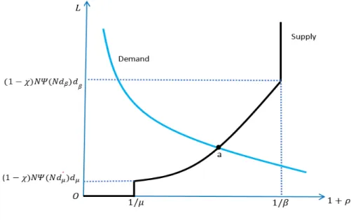
the CBDC. Equations (8) to (10) define the inverse demand function for checkable deposits. Denote it as ˆΨ to distinguish from the demand for checkable deposits without a CBDC, Ψ.
ˆ Ψ(D) =
[ µe
1+ie,∞) D= 0, µe
1+ie D∈
0,Ψ−1( µe
1+ie)
i
,
Ψ(D) D >Ψ−1( µe
1+ie).
Figure3illustrates how the CBDC changes the inverse demand for checakble deposits. The solid black line is the inverse demand with the CBDC, while the dashed line is that without
the CBDC. They overlap if the price of checkable deposits is below µe/(1 +ie). Once this
price exceedsµe/(1 +ie), the demand for checkable deposits drops to 0 after introducing the
CBDC.
4.2
Banks
To obtain the bank’s problem, simply replace Ψ(D) in (5) by ˆΨ(D). Then we can trace out the aggregate loan supply by solving the Cournot competition for all ρ such that 1 +ρ ∈
[0,1/β]. The loan supply function depends on the real gross rate of the CBDC, (1 +ie)/µe.
Letr(ρ) = 1/Ψ(N d(ρ))−1 be the real deposit rate that arises from the Cournot competition
without the CBDC. To ease the presentation, assume for now that 1/µ <(1+ie)/µe<1+rβ,
where rβ =r(1/β−1). We focus on this case because it covers all equilibrium regimes that
may occur and is sufficient to illustrate our main mechanism. Appendix A.2 provides a complete analysis of all cases.
Figure 3: Inverse Demand for Checkable Deposits
Notes. Ψ(D) is the inverse demand for checkable deposits without CBDC, and ˆΨ(D) is the inverse demand for checkable deposits with CBDC.
return of the CBDC is lower than the real rate of checkable deposits without the CBDC if
ρ >ρ.¯17 Then the equilibrium of the Cournot game stays unchanged after introducing the
CBDC because it is strictly dominated by checkable deposits.
Letρ be the loan rate at which banks break even if the deposit rate equals the CBDC rate:
(1−χ)(1 +ρ) +χ1 µ =
1 +ie
µe
.
The left hand side is a bank’s revenue from one unit of deposit. It is the sum of the revenue
from loans and that from cash reserves, weighed by the reserve requirement ratio. The right
hand side is the cost, which is the real gross interest on checkable deposits. If ρ < ρ, banks
cannot compete with the CBDC and they shut down. Then the supply of checkable deposits
and loans becomes 0.
If ρ < ρ ≤ ρ, a bank matches the CBDC rate and supplies¯ de =De/N checkable deposits,
where
De = Ψ−1
µe
1 +ie
. (11)
A formal proof can be found in Appendix A.2. Intuitively, if a bank reduces its supply of checkable deposits below de, the rate of checkable deposits remains equal to that of the
CBDC, because the latter sets a floor for the former. The deviating bank has a strictly lower
profit as the marginal profit of checkable deposits is positive, i.e.,
(1−χ)(1 +ρ) +χ1 µ >
1 +ie
µe
.
Therefore, no banks want to reduce checkable deposits. On the other hand, no banks want to increase checkable deposits because that raises interest rate and lowers profit. Notice that
by definition, d( ¯ρ) = de and the deposit supply is continuous at ρ= ¯ρ.
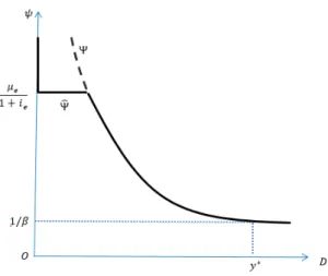
(a) Regime 1: Lowie (b) Regime 2: Medium lowie
(c) Regime 3: Medium high ie (d) Regime 4: Highie
Figure 4: Effects of a CBDC
Notes. (1) The blue curve is the loan demand, the black curve is the loan supply without a
CBDC, and the red curve is the loan supply with a CBDC. Note that the red curve joins the black
If ρ = ρ, banks are indifferent between any amount of checkable deposits in [0, de], as they
all lead to 0 profit. Also notice that if ρ ≥ ρ, banks lend up to point at which the reserve
requirement is binding.
The above analysis allows us to obtain the aggregate loan supply curve with the baseline
CBDC, shown by the solid red lines in Figure 4. The black curve is the loan supply curve without a CBDC. Again, we assume that DΨ(D) is increasing. If ρ < ρ, the aggregate
loan supply is 0. If ρ = ρ, the aggregate supply of checkable deposits can take any value
between 0 andDe. As a result, the aggregage supply of loans can be anything between 0 and
(1−χ)DeΨ(De). This corresponds to the vertical part of the solid red line. If ρ∈(ρ,ρ), the¯
aggregate supply of loans stays at (1−χ)DeΨ(De). This corresponds to the horizontal part of
the solid red line. If ρ >ρ, then the deposit rate offered by banks in the absence of a CBDC¯
is higher than the CBDC rate, and the CBDC does not affect the economy. Therefore, the
aggregate loan supply curves with and without a CBDC coincide. As ie increases, both ρ
and ¯ρ shift to the right. At the same time, the horizontal part of the red curve shifts up as
De becomes higher.
4.3
Equilibrium
The aggregrage loan demand stays unchanged and is plotted by the solid blue curves in
Figure 4. Its intersections with the solid red curve and the solid black curve correspond to equilibria with and without a CBDC.
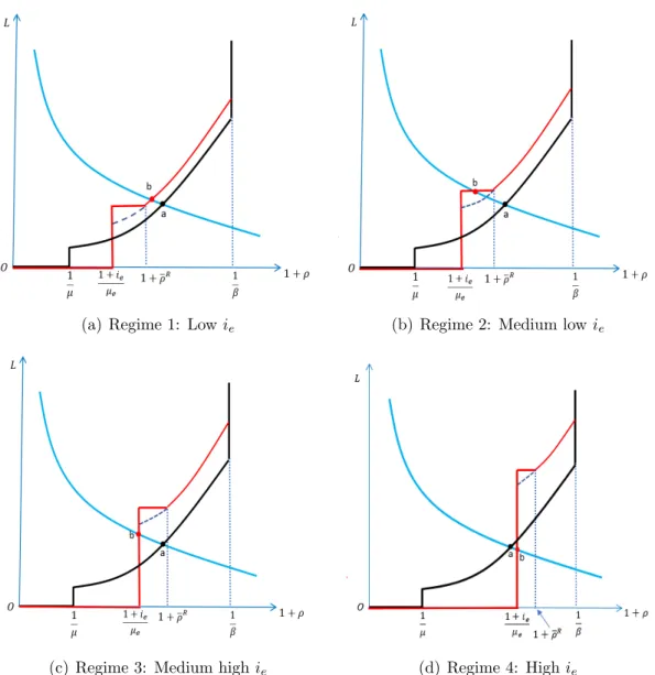
As the CBDC rate increases, the economy goes through four regimes. Regime 1 is shown in
Figure4(a). It occurs if ¯ρ < ρ∗. This is equivalent toie < ie1, whereie1solves (1+ie)/µe−1 =
r∗ and r∗ =r(ρ∗) is the equilibrium real rate of checkable deposits without a CBDC. In this
regime, the CBDC does not affect the equilibrium.
Once ie exceeds ie1, the equilibrium switches to regime 2, which is shown in Figure 4(b). Compared with the case without a CBDC, the CBDC raises the deposit rate and the demand
for electronic payment balances. If the CBDC were not introduced, banks would have
re-stricted their supply of checkable deposits and offer lower deposit rates. Because the CBDC
sets a floor for the rate of checkable deposits, this incentive is no longer active once the floor becomes effective. Moreover, the marginal profit from checkable deposits is positive if
their rate equals the CBDC rate. Therefore, banks supply De checkable deposits to meet all
the demand for the electronic payment balances at the CBDC rate, and the CBDC is not
used. A bank invests 1−χfraction of its checkable deposits on loans, so the aggregate loan
lower loan rate. A higher CBDC rate increases the rate of checkable deposits and De. It
also increases the loan quantity and decreases the loan rate. Banks then have a lower profit
margin from checkable deposits because of the higher deposit rate and the lower loan rate.
If ie = ie2, where ie2 solves (1−χ)f0(Le) +χ/µ = (1 +ie)/µe, the profit margin reaches 0
and all banks make zero profit. Notice that ie=ie2 is equivalent toρ=f0(Le)−1.
Asieincreases beyondie2, the economy enters into regime 3, illustrated in Figure4(c). Then, a higher ie increases the rates of checkable deposits and loans. In this regime, the marginal
profit from checkable deposits is 0 and banks behave as if they are perfectly competitive.
To stay break-even, banks have to increase the loan rate to compensate for a higher deposit rate. This lowers the loan demand and the equilibrium loan quantity. Banks then create
fewer checkable deposits to finance loans. However, households increase their electronic
payment balances by holding more CBDC. If the CBDC rate is lower thanie3, which solves
(1−χ)ρ∗+χ/µ= (1 +ie)/µe (or equivalently, ρ=ρ∗), introducing the CBDC still leads to
more loans and deposits.
Finally, as ie increases beyond ie3, regime 4 occurs. It is the same as regime 3 except that
the CBDC rate is too high and the quantities of checkable deposits and loans drop below the
level without the CBDC. In other words, the CBDC causes disintermediation if and only if
ie > ie3. The following proposition summarizes these discussions.
Proposition 3 Suppose that banks cannot hold the CBDC. If DΨ (D) is increasing, then there exists a unique steady-state monetary equilibrium. As (1 +ie)/µe increases from 1/µ
to 1 +rβ, the effect of the CBDC is as follows:
1. if ie ≤ie1, or ρ¯≤ρ∗, then the CBDC does not affect the economy;
2. if ie ∈(ie1, ie2), or equivalently, ρ > ρ¯ ∗ and ρ < f0(Le)−1, then the CBDC increases
lending relative to the case without a CBDC, and a higher ie increases lending;
3. if ie ∈(ie2, ie3), or equivalently, ρ > ρ¯ ∗ and ρ > f0(Le)−1, then the CBDC increases
lending relative to the case without a CBDC, and a higher ie reduces lending;
4. if ie > ie3, or equivalently, ρ∗ < ρ¯, then the CBDC decreases lending relative to the
case without a CBDC, and a higher ie reduces lending.
Our analysis delivers three important messages. First, introducing a CBDC does not
nec-essarily cause disintermediation and reduce bank loans and deposits. Indeed, the CBDC
expands bank intermediation by introducing more competition to the banking sector if its
Second, one should not judge the effectiveness of the CBDC on its usage, but rather on how
much it affects the deposit and the lending rates or quantities. Throughout regime 2, the
CBDC is not used, but increases both deposits and loans. In fact, it maximizes lending if
ie =ie3, which is in regime 2. Here, the CBDC works as a potential entrant. It disciplines the off-equilibrium outcome: if banks reduce their real deposit rates below the real CBDC
rate, then buyers would switch to the CBDC.
Third, there can be a trade-off between payment efficiency and the investment quantity. In
regimes 3 and 4, both the CBDC and checkable deposits are used as means of payment. If
the CBDC rate is higher, households hold more electronic payment balances. This allows them to consume more in the DM. But at the same time, the loan rate increases and loan
quantity falls. For more discussions, see Keister and Sanches (2019).
We end this section with a comparison between an interest floor policy and the CBDC. They
share some similarities but the CBDC in general delivers better outcomes. If the CBDC rate
ie is lower than ie2, the CBDC is not used. Then the effect of a CBDC is identical to a
policy that mandates banks to pay a real rate no less than (1 +ie)/µe−1. If, however, ie is
larger thanie2, households use the CBDC for transactions, because the banks do not create
enough checkable deposits to satisfy the transaction needs. With an interest floor policy,
the CBDC is not available to households any more. As a result, households have lower electronic payment balances and consume less in the type 2 and 3 meetings. This reduces
welfare. In fact, the equilibrium under a CBDC withie larger thanie2 cannot be achieved by
any interest floor policy, because the latter does not provide additional electronic payment
balance to meet the demand.
5
CBDC as Reserves
Now we modify the baseline design to allow banks to hold the CBDC as interest-bearing reserves, i.e., the CBDC can be used to satisfy the reserve requirement. The CBDC now
plays two roles. First, it is a means of payment that competes with checkable deposits.
Second, it can lower the cost for the banks to hold reserves if it has a higher return than
cash.
bank’s problem changes to
max
ze j,zj,`j,dj
(1 +ρ)`j+
zj
µ +
(1 +ie)zje
µe
−dj
s.t. `j+zj +zej = ˆΨ (d−j +dj)dj,
zje+zj ≥χΨ (dˆ −j+dj)dj,
whereze
j is bankj’s CBDC balance. As before, we solve the Cournot game among banks for
each value of ρ and trace out the aggregate loan supply.
To solve for the equilibrium in this Cournot game, we adopt a two-step approach that
parallels the one used for the baseline CBDC. In the first step, we solve the equilibrium of
an auxiliary model where only banks can hold the CBDC. This shuts down the role of the CBDC as a competing means of payment. It is similar to the model without a CBDC. The
only difference is that banks may earn the CBDC rate on their reserves. The second step
parallels the analysis in Section 4.2. We compare the real rate of checkable deposits in the auxiliary model with the real CBDC rate. If the former is higher, the equilibrium of the
original Cournot game is the same as the equilibrium of the auxiliary model. Otherwise, we
adjust the deposit and loan supply in a similar way as in Section 4.2. The details can be found in Appendix A.3.
The red curves in Figure 5 illustrate the resulting aggregate loan supply curve. Again, we assume thatDΨ(D) is increasing. Same as in Figure4, the aggregate loan supply curve with the CBDC coincides with the horizontal axis ifρis low. Ifρis intermediate, the curve is flat.
The deposit rate matches the CBDC return, and the quantity of loans is fully determined
by the CBDC rate and equals (1−χ)DeΨ(De). If ρ is above a cut-off ¯ρR, the return of
the CBDC is lower than that of checkable deposits, and the aggregate loan supply curve is
upward sloping.
Compared with the baseline design, besides being an alternative payment method (payment competition effect), the CBDC can also reduce the bank’s cost to hold reserves (cost-saving effect). The two effects together shift the loan supply curve without a CBDC, shown by the solid black curve, to the one with the CBDC. To decompose these two effects, we also plot
the aggregate loan demand curve in the auxiliary model, where we shut down the payment
competition effect. It is the dashed blue curve on ((1 +ie)/µe,1 + ¯ρR) but overlaps with the
red curve otherwise. The shift from the solid black curve to the dashed curve captures the
competition effect.18
Similar to the baseline design, the equilibrium can be classified into four regimes. These
regimes are separated by three cut-offs in the CBDC rate iR
e1 < iRe2 < iRe3. Both the regimes and cut-offs parallel those under the baseline CBDC design.
Figure 5(a) shows regime 1, which occurs if ie < iRe1. The loan demand curve (the solid blue curve) intersects the loan supply curve with the CBDC in its increasing region. Buyers
strictly prefer bank deposits to the CBDC and the payment competition effect is not
oper-ative. However, the cost-saving effect is still present. If the CBDC offers a higher return
than cash, it reduces the cost to hold reserves. As a result, the bank supplies more check-able deposits and loans (point b), and the equilibrium loan rate is lower compared with the
equilibrium without the CBDC (point a). In this regime, a higher ie decreases the cost of
holding reserves; hence it increases the deposit rate and the quantities of deposits and loans.
It also reduces the loan rate.
As ie increases beyond iRe1, the equilibrium switches to regime 2, illustrated by Figure 5(b). Same as in the baseline design, all banks together issue De checkable deposits to absorb all
the demand for the electronic payment and the CBDC is not used. As the CBDC rate rises,
the equilibrium rate and quantity for checkable deposits rise, and the amount of loan supply increases and the loan rate decreases. This reduces the bank’s profit margin. Onceie reaches
iR
e2, the bank profit becomes 0.
If ie exceeds iRe2, the economy enters into regime 3, shown in Figure 5(c). Same as with the baseline design, banks earn zero profit in this regime. A higher ie raises the deposit and
loan rates, and lowers the loan quantity.19 Households use both checkable deposits and the
CBDC for transactions. As ie further increases to iRe3, the loan quantity decreases to the
level when there is no CBDC.
As ie increases beyond iRe3, the economy enters into regime 4 shown in Figure 5(d). This is the only regime in which the CBDC causes disintermediation relative to the case without a
18In the increasing part of new (red) loan supply curve (ρ∈[ ¯ρR,1/β−1)), the payment competition effect
is muted, and the higher loan supply relative to the old (black) supply curve is due to the cost-saving effect. In contrast, with the baseline CBDC design, the cost-saving effect is absent and the loan supply curves with and without the CBDC coincide with each forρ∈( ¯ρ,1/β−1)).
(a) Regime 1: Lowie (b) Regime 2: Medium lowie
(c) Regime 3: Medium highie (d) Regime 4: High ie
Figure 5: CBDC as Reserves
Notes. (1) The blue curve is the loan demand, the black curve is the loan supply without a CBDC, the dashed black line is the loan supply when a CBDC is used as reserves but cannot be used for payments, and the red curve is the final new loan supply with a CBDC that can be used for both reserves and payments. The dashed line coincides with the red curve except for
ρ∈ (1 +ie)/µe,ρ¯R
CBDC. As the CBDC rate continues to rise, the response of the economy is the same as in
regime 3. In both regime 3 and regime 4, a higher CBDC rate improves payment efficiency
at the cost of investment.
To summarize, a CBDC that serves as reserves can also promote bank intermediation.
Com-pared with the baseline CBDC, it has the additional cost-saving effect. This effect can be
active and increases lending even if the CBDC has a lower rate of return than checkable
deposits. Therefore, this design can increase bank intermediation more compared to the
baseline design. Moreover, it promotes bank intermediation for a wider range of ie than the
baseline CBDC. Also notice that iRe1 ≥ ie1. Because of the cost-saving effect, banks offer a higher rate on checkable deposits than under the baseline design. Then, a higher rate is
necessary for the CBDC to be a competitive payment method. Similarly, a higher CBDC
rate is needed to drive the bank profit to 0, i.e., iR
e2 ≥ie2.
6
Quantitative Analysis
Theoretically, the CBDC can increase bank lending if its interest rate lies in a certain range.
They remain empirical questions how large this range is and how big the effect of the CBDC can be. These questions are important for policy decisions. We calibrate our model to the
U.S. economy between 2014 and 2019, and then conduct a counterfactual analysis to answer
these questions. We also study the effects of a non-interest bearing CBDC if the economy
trends towards cashless.
6.1
Calibration
We introduce two modifications to the model. First, we assume that banks incur a
man-agement cost c per unit of deposits.20 In our model, this is equivalent to a variable asset
management cost. Second, we allow sellers in the DM to have market power. Specifically,
in the DM, the terms of trade are determined by Kalai bargaining with bargaining power
θ to the buyer. These two modifications do not affect the qualitative analysis but capture
two features in the data: sellers have substantial markups and banks have operational costs. Both features can be quantitatively important.
Consider an annual model and the functional forms U(x) = Blogx, u(y) = [(y+)1−σ −
1−σ]/(1−σ), and f(k) = Akη. The parameter is set to 0.001. It is introduced to
guarantee u(0) = 0 so that the Kalai bargaining is well-defined for all σ. It has little effect
20This adds the term−c(ψd+ψ
on our counterfactual analysis. To simplify presentation, define Ω = α1 +α2 +α3 as the
trading probability of a buyer.21 Define ˆα
i =αi/Ω, i = 1,2,3, as the probabilities of being
in a typeimeeting conditional on being matched with a seller. We can then replaceαi with
Ω and ˆαi. There are 14 parameters to calibrate: (A, B, N,Ω,αˆ1,αˆ2,αˆ3, σ, c, θ, β, η, χ, µ).
Eight parameters, β, η, µ, χ,αˆi(i = 1,2,3), and c, are set directly. The rest are calibrated
internally. We assume that (Ω, B, σ, η) are stable over time. This allows us to use time series
data from early years for calibration. For ˆα1,αˆ2,αˆ3, c, A, N and µ, we use only data between
2014 and 2019 because they may vary over the time.
We use four data sets in this exercise: (1) Survey of Consumer Payment Choice (SCPC) and Diary of Consumer Payment Choice (DCPC) from the Federal Reserve Bank of Atlanta; (2)
call reports data from FFIEC; (3) new M1 series from Lucas and Nicolini (2015); and (4)
several macro series from FRED. In what follows, we briefly discuss the calibration of several
key parameters. For details, see Appendix E.
We obtain the ˆαs from SCPC and DCPC from the Federal Reserve Bank of Atlanta. The
SCPC contains information on the fraction of online transactions and the DCPC contains
information on the perceived fraction of point-of-sale transactions that do not accept cash or
debit/credit cards. We use the data from the 2016 wave and the numbers are similar in 2015
and 2017. The SCPC documents that an average household makes 67.8 transactions per month. They include 6.6 automatic bill payments, 5.9 online bill payments and 4.7 online
or electronic non-bill payments. We count these as online transactions and they represent
25.37% of all transactions. We assume that all the online transactions accept only deposits.
At the point of sale, the DCPC reports that 15% transactions do not accept debit/credit card
and 2% transactions do not accept cash. Then, cash-only transactions are those at points of
sale that do not accept cards. This implies ˆα1 = 15%(1−25.37%) = 11.19%. Deposit-only
transactions include online transactions and point-of-sale transactions that do not accept
cash. Hence, ˆα2 = 25.37% + 2%(1−25.37%) = 26.86%. And ˆα3 = 1−αˆ1−αˆ2 = 61.94%.
Next, calibrate (Ω, σ, B) using the standard approach of matching the money demand curve.
We use the new M1 series from Lucas and Nicolini (2015). This data include checkable
deposits and some interest-bearing liquid accounts. To calculate the money demand in
the model, we also need the deposit rates. The call reports data, which was also used in
Drechsler et. al (2017) and Drechsler et. al (2018), contain balances and interest expenses
on transaction accounts of US banks. We take the ratio of these two variables to obtain an
average interest rate on transaction deposits. For this calibration, we use data from 1987
to 2008. Before 1987, interest expenses on transaction accounts are not available. After the
financial crises, demand for M1 rises sharply likely due to non-transactional demand, such as
store-of-value or foreign demand. Because our model focuses on the transactional demand,
it is more reasonable to exclude the post-crisis data.22 Notice that in this exercise, we set the
ˆ
αs to their values in 2016. It is possible that their values change during 1987-2008 and may
be different from the values in 2016. However, our approach remains valid if the changes
in the ˆαs affect mainly the composition of M1, but not the its aggregate, which includes
both cash and checkable deposits. This assumption is consistent with data, i.e., the money
demand curve is stable during 1987-2008.
Set η to match the elasticity of commercial loans with respect to the prime rate using the
time series from FRED. Givenη, choose (A, c, N) to hit several targets in the banking sector
between 2014 and 2019, which are computed from the call reports data. We choose c to
match the average non-interest expenditures excluding expenditures on premises or rent per
dollar of assets. Set A to match the average interest rate on transaction accounts. Pick N
to match the spread between the loan rate and the rate on transaction accounts.
Table1summarizes all the parameter values.23 Figure6(a)shows the model-predicted money demand curve against the data between 1987 and 2008. The model fits the data well. Figure
6(b) shows the loan supply and loan demand as functions of 1 + ρ under the calibrated parameters. The loan supply curve is monotone and the equilibrium is unique.
6.2
Effects of a CBDC on Banking
Now we introduce a CBDC that is a perfect substitute for checkable deposits. We consider
both the baseline design, and the modified design where the CBDC serves as reserves. The
supply of the CBDC grows at the same rate as cash. We focus on how the CBDC affects the
economy with different interest rates. We are particularly interested in lending and output.
Figure 7 shows the results. The first row displays percentage changes of deposits, loans and total output relative to the equilibrium without the CBDC. The second row shows
22We have also done a calibration with data between 1987 and 2019. The increased money demand leads to a larger DM. As a result, the CBDC has a bigger impact. For example, the baseline CBDC can increase loans up to 2.09% and output up to 0.34%. It promotes bank intermediation for a slightly wider range of rates compared to the results reported later in this section.
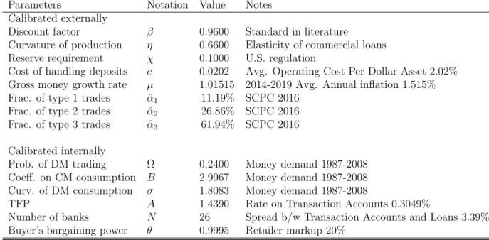
Parameters Notation Value Notes Calibrated externally
Discount factor β 0.9600 Standard in literature
Curvature of production η 0.6600 Elasticity of commercial loans Reserve requirement χ 0.1000 U.S. regulation
Cost of handling deposits c 0.0202 Avg. Operating Cost Per Dollar Asset 2.02% Gross money growth rate µ 1.01515 2014-2019 Avg. Annual inflation 1.515% Frac. of type 1 trades αˆ1 11.19% SCPC 2016
Frac. of type 2 trades αˆ2 26.86% SCPC 2016 Frac. of type 3 trades αˆ3 61.94% SCPC 2016
Calibrated internally
Prob. of DM trading Ω 0.2400 Money demand 1987-2008 Coeff. on CM consumption B 2.9967 Money demand 1987-2008 Curv. of DM consumption σ 1.8083 Money demand 1987-2008
TFP A 1.4390 Rate on Transaction Accounts 0.3049%
Number of banks N 26 Spread b/w Transaction Accounts and Loans 3.39% Buyer’s bargaining power θ 0.9995 Retailer markup 20%
Table 1: Calibration Results
(a) Model Fit (b) Equilibrium
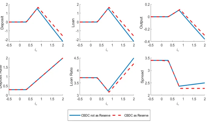
Figure 7: Effects of CBDC Rate
deposit and loan rates and their difference, i.e., the spread. All rates are nominal and in
percentages. The solid blue curve is under the baseline design, and the dashed red curve is
under the modified design.
Let us start with the quantities of checkable deposits and loans. First, focus on the economy
with the baseline CBDC. If ie is lower than 0.30%, which is the deposit rate without the
CBDC, the rate of the CBDC is below that of checkable deposits. The economy stays in
regime 1. The CBDC is not used and has no effect on the economy. As ie increases, we see
the first kink in the deposit quantity curve, which leads to the first kink in the loan quantity curve. Then the economy enters regime 2. The competition effect is active and leads to more
deposits and loans. An increase in ie significantly increases checkable deposits and loans.
If ie is sufficiently high, then deposits and loans start to decrease and the economy enters
regime 3. If ie is above 1.28%, checkable deposits and loans drop below their levels without
a CBDC and the economy enters regime 4. Relative to the economy without a CBDC, the
baseline CBDC increases lending if its rate is between 0.30% and 1.28%. At the maximum,
it increases lending by 1.53%.
If the CBDC also serves as reserves, its effect on deposits and loans is stronger than the
deposits and loans if 0< ie <0.30%. In this region, the dashed red curve is slightly above
the solid blue curve. If ie becomes larger, the competition effect becomes active. Because
banks satisfy all the demand of electronic payment balances at the CBDC rate, the checkable
deposit and loan quantities are the same under both CBDC designs. The solid blue and the
dashed red curves overlap. Because of the cost-saving effect, the dashed red curve starts to
decline at a biggerie and is always above the solid blue curve for sufficiently large ie. Under
this design, the CBDC increases bank intermediation ifie is between 0% and 1.43%. At the
maximum, it increases lending by 1.67%.
Notice that the competition effect is more important than the cost-saving effect because of two reasons. First, the competition effect applies to all checkable deposits, while the
cost-saving effect applies only to the reserves, which is at most 10% of all checkable deposits.
Second, banks may not fully pass the cost-saving effect to the economy because of their
market power.
Now we turn to the interest rates and the spread. The deposit rate is shown in the first
panel in the second row. With the baseline CBDC, the deposit rate is constant ifie is below
0.30% and coincides with the 45o-line once theie exceeds the deposit rate in the absence of a
CBDC. This reflects that the CBDC rate serves as a floor of the deposit rate. If the CBDC
serves as reserves, it has the additional cost-saving effect. Therefore, a higher ie increases
the the deposit rate if 0< ie <0.30%. But this effect is very small.
The loan rate reverses the pattern of loans, as shown in the second panel. If ie is set
appropriately, then the loan rate reduces to around 3.17% from about 3.7%. If ie is too
high, then the loan rate can be higher than in the equilibrium without a CBDC, which hurts
lending.
The spread, defined as the nominal lending rate minus the nominal deposit rate, is shown
in the third panel in the second row. The CBDC reduces the spread by competing with
checkable deposits. Ifieis sufficiently high, banks act as if the market is perfectly competitive.
Then, the lending rate equals the marginal cost of lending, which includes the interest paid
on deposits, the cost of handling deposits, and the cost of holding reserves.24 With the
baseline CBDC, the spread increases with the CBDC rate. This is caused by the higher cost
of holding reserves because the difference between the deposit rate and the return on cash
reserves increases. This difference disappears if the CBDC serves as reserves, and the spread