Extrasolar planet detection through spatially resolved observations

(1)

The handle http://hdl.handle.net/1887/33272 holds various files of this Leiden University

dissertation.

Author: Meshkat, Tiffany

(2)

Through Spatially Resolved Observations

Proefschrift

ter verkrijging van

de graad van Doctor aan de Universiteit Leiden,

op gezag van de Rector Magnificus Prof. mr. C. J. J. M. Stolker, volgens besluit van het College voor Promoties

te verdedigen op donderdag 11 juni 2015 klokke 15:00 uur

door Tiffany Meshkat

(3)

Promotor: Prof. dr. I. Snellen Co-promotor: Dr. M. Kenworthy

Overige leden: Dr. B. Biller (University of Edinburgh) Dr. D. Stam (TU Delft)

Dr. M. Hogerheijde Prof. dr. C. U. Keller Prof. dr. H. V. J. Linnartz Prof. dr. H. J. A. R¨ottgering

ISBN: 978-94-6259-708-2

Cover: Artist impression of a directly imaged planet in a debris disk.

Designed by Tiffany Meshkat and Joshua Routh.

(4)

(5)

of our answers.”

(6)

Chapter

1

Introduction

The interest in extrasolar planets (exoplanets) has been a feature of human inquiry for thousands of years, as evidenced by Epicurus’ letter to Herodotus in the 4th century B.C. where he postulated that many other worlds – similar and different to our own – must exist. This curiosity is very relatable: we want to better understand ourselves, our planet, and our place in the universe. Until fairly recently, the only known planets were in our own solar system. Much of star and planet formation theories were derived from this limited knowledge. The existence of exoplanets was only confirmed when indirect planet detection techniques became suitably sensitive to find planets (Wolszczan & Frail 1992;Mayor & Queloz 1995).

The earliest exoplanet detection technique, radial velocity, takes advantage of the subtle Doppler shift in a star’s spectrum due to a massive body orbiting nearby. This gravitational “wobble” technique revealed hundreds of close-in planets with systems very different to our own. The existence of “Hot Jupiters”, planets as massive as Jupiter but within Mercury’s orbit, led to a whole new field of planet migration studies. Later on, the transit technique led to the discovery of hundreds more planets which, by chance alignment with Earth, block out a small amount of the light from a star, causing a dip in its light curve over time. Since then, technological developments both from the ground and space, have resulted in the discovery of >1500 confirmed planets1_{, in a diverse range of architectures and}

masses. The size and distribution of exoplanets around nearby stars in our galaxy provides insight into the different types of planet formation. This ultimately can help to reveal if our Solar System is typical or an exception.

(11)

N

E

L_′ Clio

E 1"

N

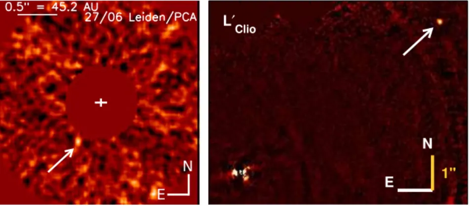
Figure 1.1 Left: Directly imaged 5 Jupiter mass planet HD 95086 b fromRameau et al.(2013c), indicated with a white arrow. Right: Planet HD 106906 b (white arrow)L0-band detection fromBailey et al.(2014).

1.1 Directly Imaging Exoplanets

Direct imaging is a recently successful technique to detect and characterize exo-planets. It involves directly detecting the photons from a planet itself. This techniques provides a unique opportunity to study young planets in the context of their formation and evolution. It examines the underlying semi-major axis exo-planet distribution (5 to 100 AU) and enables the characterization of the exo-planet itself with spectroscopic examination of its emergent flux (Konopacky et al. 2013). This method of planet detection is challenging for several reasons, some of which are readily apparent (planets are small, faint, and close to their host star) and others which are less clear from the outset (such as wavefront control, quasi-static speckles, etc. see Section1.4). The limits of current technology only allow the direct detection of young, self-luminous planets. These young planets are still warm from their contraction, making them easier to directly detect in the infrared (Burrows et al. 2004) with typical planet-to-star contrasts of10−5−10−6, compared to the values of10−9₋₁₀−10_{for more mature planets. Since these planets are young,} they are ideal candidates to study the late stages of planet formation.

(12)

0.01 0.1 1 10 100 10

1

0.1

0.01

10-3

Separation [Astronomical Units (AU)]

Planet Mass [J

upiter Mass]

exoplanets.org

Radial Velocity

Transits

Microlensing

Direct Imaging

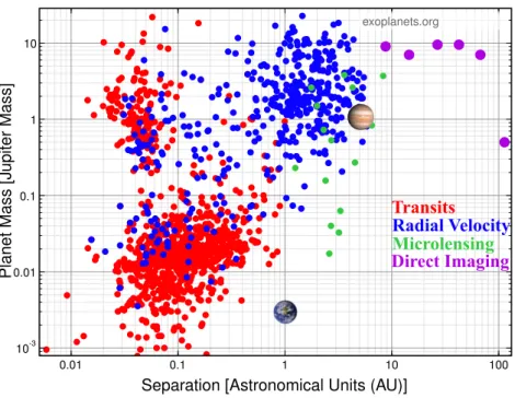
Figure 1.2 All detected and confirmed planets shown as a function of planet-star separation in AU and Jupiter masses (from exoplanets.org). The different colored points denote the method the planet was originally detected in. The vast majority of planets have been detected through the transit (red) and radial velocity (blue) method. Directly imaged planets (purple) are at a wider separation and higher mass than those detected through other techniques. Earth and Jupiter are also included as reference points.

(13)

1.2 Planet Formation

Stars are formed from large cold clouds of molecular gas. Gravitational instability perturbs the cloud and starts its collapse. As a star forms out of a molecular cloud (Bergin & Tafalla 2007), conservation of angular momentum flattens its surrounding dust and gas into a circumstellar disk. It is in this early, gas rich stage that planets are thought to form. Eventually the gas is depleted, either blown out into the interstellar medium through stellar winds or through accretion onto the star or a planet (Alexander et al. 2014). The final stage in the disk life around a star is the debris disk phase, where planetesimals are collisionally ground up to form dust that is seen in reflected light (reviews byWyatt 2008;Matthews et al. 2014). The planets in debris disks are thus recently formed, but the formation mechanism of giant planets is still a matter of contention. Even Jupiter’s interior (and thus formation mechanism) is not well understood (Guillot 2005;Fortney & Nettelmann 2010). Two of the most popular giant planet formation mechanisms are core accretion (Safronov & Zvjagina 1969; Hayashi 1981;Pollack et al. 1996) and gravitational instability (Boss 1998;Mayer et al. 2002).

Core accretion begins with small micron and centimeter sized particles in a disk colliding and sticking together to form larger particles. These particles eventually coagulate to form planetesimals, which accrete to form a rocky planetary core (∼5−10M⊕). As this planetary core orbits the star, its gravity accretes gas onto

the surface of the core in a runaway process. This sweeping-up process also may explain how planets migrate through a disk. Planetary migration is a process which must have occurred given the observations of “Hot Jupiters” , which are too massive to have formed and swept-up enough gas at their current, small orbital separations (Lin et al. 1996;Rasio et al. 1996). However, this formation method is not without its challenges. Meter sized particles are expected to collide at velocities that are too high to result in sticking (Brauer et al. 2008). These bodies also decouple from the gas, causing them to drift rapidly into the star (Weidenschilling 1977). These two processes make it difficult for particles to grow larger than a meter in size. Icy dust grains have been proposed as a method to overcome this barrier, as ice grains collide and stick more easily (Okuzumi et al. 2012; Krijt et al. 2015). Also, accretion of gas onto the core must occur before the disk dissipates. Core accretion is thought to occur on a timescale of 0.5 to 10 Myr, while the observed disk lifetimes are 1 to 10 Myr.

Gravitational instability is a “top-down” method of giant planet formation. A higher mass planet is thought to form out of an instability in the gas and dust rich disk, which fragments into clumps and starts a gravitational collapse (Boss 1998;Mayer et al. 2002). In this scenario, the dust grains sink to form the core of the planet via self-gravity. Unlike core accretion, gravitational instability can form planets relatively quickly, with a timescale of a few disk orbits (100-1000 years at 10 to 100 AU). However, the cause of the fragmentation is uncertain. Fragmentation can only occur if the disk cools quickly enough, based on the Toomre instability parameter, or it can be caused by an external gravitational trigger, such as a binary star (Mayer et al. 2005).

(14)

Cool Kuiper Belt

Jupiter

Saturn

Uranus

Neptune

Warm Asteroid Belt

Figure 1.3 Left: The debris disk around the star Fomalhaut (Kalas et al. 2005), seen with the Hubble Space Telescope in scattered light. The debris has been sculpted into a ring, likely by an unseen planet. Right: Visualization of the two-belt dust debris structure in the Solar System.

planets in different parts of the disk: gravitational instability beyond a disk radii

r>100 AU and core accretion insider<100AU. Transit studies with the Kepler space telescope have revealed that small planets (≤2.5R⊕) are extremely common

at small angular separations (Batalha et al. 2013;Fressin et al. 2013;Lissauer et al. 2014). Given their current separation and relatively low mass, most of these planets are thought to have formed via core accretion. Direct imaging surveys suggest that planets are very infrequent at large separations (see Section 1.5). These large separation, high mass planets have been proposed to form by gravitational instability (Marois et al. 2010). However, recent studies cast doubt on the HR 8799 planets having formed via gravitational instability, as their masses and separations do not fulfill the model Toomre and cooling time criteria (Rameau et al. 2013a). Additionally, the lack of giant planets at large orbital radii suggests that giant planets formed via gravitational instability are uncommon (Bowler et al. 2015).

Theoretical planet cooling curves are employed to predict the temperature of giant planets over time. The “hot-start” models (Burrows et al. 1997) are most closely related to the gravitational instability planet formation mechanism: an object radiates its initial gravitational potential energy slowly. The “cold-start” and “warm-start” models (Marley et al. 2007; Spiegel & Burrows 2012) involve the rapid loss of initial entropy caused by accretion, and thus is more related to core accretion. The masses of directly imaged planets are estimated from these evolutionary models.

1.3 Planet-Disk Interactions

(15)

Figure 1.4 24µm excess emission versus age for A-type stars, from (Rieke et al. 2005). The excess emission is the ratio of the flux density in the SED over the stellar photosphere alone. A ratio of 1 has no excess emission. Targets with an excess ratio >1.25 are considered the threshold for detection of an excess. An excess ratio >2 is considered a large excess. The decaying frequency of debris disks with age demonstrates the likelihood that an A-type star with a debris disk is young.

asteroids and comets, which can form grains down to a few microns (Acke et al. 2012). These small bodies are the remnants of planetesimals, which are thought to be the building blocks of planet cores. Thus, debris disks may be indicators of recent planet formation.

Debris disks can be directly detected (Figure 1.3, left) or inferred from ex-cess infrared emission in a stellar energy distribution (SED). Resolved debris disks are extremely useful for direct imaging studies, as the inclination of the system can be assessed and, in some cases, substructure (such as gaps or holes) can be seen (Kalas et al. 2005). If a companion is detected in such systems, the inclina-tion allows determinainclina-tion of the orbital separainclina-tion from the star, rather than the projected separation. For unresolved debris disks, the approximate mass, temper-ature, inner and outer radii can be inferred by fitting the SED with an appropriate model. Figure1.4demonstrates that the frequency of debris disks decays over time (Rieke et al. 2005). These debris disks are inferred from excess 24µm emission in their SEDs. Whether the disk is resolved or not, debris disks provide a wealth of information about the structure of the dust around a star and imply youth for the system.

(16)

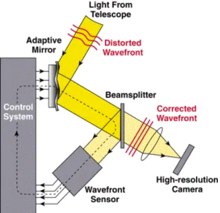
Figure 1.5 Demonstration of how an AO system corrects an incoming wavefront using a wavefront sensor which then adjusts the deformable mirror in real-time to produce a final corrected image (lyot.org).

four planets present across the gap (Figure1.3, right). In the case of Fomalhaut, the cool outer belt is resolved, while the warm inner belt is inferred from the SED.

1.4 Observing Strategies and Image Processing

1.4.1 Optical Aberrations

As the light from a point source passes through an optical system, the shape of the image is called the point spread function (PSF). In the case of a circular aperture in a telescope, the PSF shape is described as an Airy disk. The central core of the PSF contains most of the stellar flux, with several, successively fainter Airy rings around the star. The theoretical, diffraction-limited resolution of a telescope is defined on this basis:

(17)

Achieving the diffraction limit of a telescope, however, is a challenging task. Instrumental aberrations are present in nearly every optical system. Even the Hubble Space Telescope has spherical aberrations in the primary mirror. In addi-tion to static instrumental aberraaddi-tions, ground-based telescopes have the challenge of observing through the turbulent, refractive atmosphere of the Earth.

1.4.2 Adaptive optics

The Earth’s atmosphere introduces temporal and spatial variations in the light path from a point source, causing an image to appear smeared out. Adaptive Op-tics (AO) was invented in order to counter this blurring. An AO system measures the deviations in the incoming stellar wavefront using a wavefront sensor. The wavefront sensor determines the correction necessary to create a flat wavefront, and sends the correction information to a deformable mirror (DM). Ideally the DM cancels the aberration in the wavefront by physically reshaping the mirror, using actuators, to be the inverse aberration shape with half the amplitude. In a theoretical system where the DM is able to correct the atmospheric aberrations in real-time, the resulting wavefront would be flat. In practice, there is a brief time delay between the wavefront sensor and the DM correction. This process is repeated hundreds of times a second in order to compensate for the varying turbulence, which produces a point source (seeFigure 1.5).

In order for this process to measure the wavefront accurately, a bright light source is needed. If the target object is too faint to be a natural guide star, a laser guide star is used to generate a fake point source. For the purposes of directly imaging exoplanets, the target stars are most often bright enough to act as their own natural guide star. AO correction is necessary to directly image exoplanets, since we require the stellar flux to be centralized in a point source as much as possible, in order to detect faint point sources at very small angular separations.

1.4.3 Coronagraphs

Coronagraphs are optics inserted in the light path of a telescope which minimize the diffracted light from a source, to allow access to small angular separations around a star. One of the first coronagraphs, the classical Lyot (Lyot 1939), achieved this with two optical elements, visualized in the top light path diagram inFigure 1.6. The light from the star (blue line) is blocked by a mask in the focal plane of the telescope. Since the planet (red line) is physically separated from the star, the angle of its incoming light is not blocked by the mask. Then a Lyot stop is inserted in the pupil plane in order to block the outer edge of the telescope pupil in the pupil plane image. Finally the image is formed on the detector. This coronagraph design is extremely sensitive to the telescope alignment, as the star must be placed precisely behind the focal plane mask (called tip-tilt alignment) and is thus sensitive to telescope vibrations. This physical mask also has the potential to block a planet signal, which may be very close to its parent star. Developments in coronagraphs have led to significant improvements on the classical Lyot (4QPM;

(18)

Figure 1.6 Light path diagrams demonstrating the Lyot coronagraph and the APP coronagraph designs, from Kenworthy et al. (2010). Both coronagraphs aim to allow the detection of faint sources close to a bright star. The classical Lyot uses a focal plane mask and a Lyot stop in the pupil plane. The APP only has one optic, which is in the pupil plane. The resulting image on the detector is seen on the right.

designs require an optic in the focal plane.

The Apodizing Phase Plate (APP) coronagraph (Kenworthy et al. 2010) uses only a single optic, placed in the pupil plane of the telescope, seen in the bottom light path diagram inFigure 1.6. The APP optic uses the light diffracted from the Airy core of the star to cancel out the coherent light in the diffraction rings. In effect, this minimizes the diffraction pattern on one side of the star, while reinfor-cing it on the other side. The result is seen on the right ofFigure 1.6, the central Airy core of the star still reaches the detector, but the adjusted diffraction ring pattern allows the planet signal to shine through. This figure also demonstrates that everything in the field of view will have the characteristic APP diffraction suppression structure, including planets. As the central Airy core flux itself is used to cancel out the diffraction pattern on one side of the star, there is a cost of 40% to throughput. The APP was designed to have a “dark hole” where the sky background limit can be reached in the final APP images from000.₁₈_to ₀00_.₇₅

in which to search for faint companions. The most significant difference with pre-vious coronagraph design is the lack of a focal plane mask. Thus, the APP is insensitive to tip-tilt errors and can even be used to observe binary star systems.

(19)

✁

✂

✄

☎✆

☎☎

✝✞✞

✟✠✡☛☞✌

✆✍✎ ✆✍✏ ✆✍ ✆✍✂ ☎✍✆ ☎✍✎

✑✒✓✔✕✖ ✗✒✘✙✖✚✙✛

✜

✢

✣

✤

✥

✦

✧

★

✩

✪

✫

✦

✢

✪

✬

✥

✦

✤

✭

✮ ✯✰✱✲ ✯✳✴

✵ ✶ ✷ ✸ ✹✺ ✹✵ ✹✶

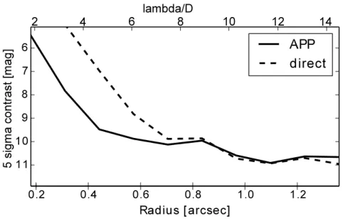
Figure 1.7 Comparison of sensitivity achieved with the APP coronagraph versus direct imaging for the same target observed with the NACO instrument on the VLT (from Meshkat et al. submitted).

NACO instrument on the VLT and processed with these same pipeline.

1.4.4 Angular Differential imaging

Sophisticated image processing algorithms are necessary to remove the “quasi-static super speckles” in our data, in order to let the light from a planet shine through. Though direct imaging data are obtained with AO correction, speckles remain in the images. These speckles, caused by instrumental features and residual atmospheric turbulence, can appear brighter than a planetary-mass companion (Hinkley et al. 2009). Several image processing algorithms have been developed to model and subtract these aberrations. One such algorithm is Angular Differential Imaging (ADI:Marois et al. 2006). In ADI mode, the sky de-rotator on an ALT-AZ mounted telescope is turned off, allowing the sky to rotate around a star. A planet will appear to orbit over time, while the aberrations stay relatively fixed. Assuming the planet is not in the same position in any consecutive images, a median over all images in time will capture the static speckle aberrations, but not the planet. While this median image succeeds in modelling the general stellar PSF structure, the speckles vary in brightness on time scales of the observing sequence.

1.4.5 SDI

(20)

Differential Imaging (SDI) is a method which takes advantage of this prediction, by simultaneously imaging in and out of the methane absorption feature at 1.62

µm. By subtracting the different narrow-band images, the stellar flux and speckles will be subtracted and the light from planet with methane absorption will be preserved (Biller et al. 2007). However, many recent studies do not find strong methane absorption from the known directly imaged planets (e.g. HR 8799 bcd and 2M1207 b;Skemer et al. 2014), suggesting that planets are not the same as field brown dwarfs of equivalent effective temperatures.

1.4.6 Locally optimized combination of images

Locally Optimized Combination of Images (LOCI) (Lafreni`ere et al. 2007) is a planet detection algorithm which models the stellar PSF in a subregion of the im-ages to remove speckles. Data are obtained in ADI mode, to allow any companion source (and the sky) to rotate between successive images in time. For the ADI algorithm a simple median is taken over all the images in order to subtract the stellar PSF. This assumes that there is enough sky rotation such that a companion will never overlap with itself in successive images. In practice, a companion will always have some small amount of overlap between images. Thus, subtracting the median of the images will result in some self-subtraction of a companion. The LOCI algorithm mitigates this problem by introducing the parameterNδ, which is

the minimum amount of overlap allowed in units of the PSF full-width half max-imum (FWHM). This determines how many images are rejected from the stellar PSF fit, in order to prevent self-subtraction. For example, anNδof 1 ensures there is no overlap of a companion, however it may result in the rejection of many frames depending on the sky rotation and angular separation of a companion. At smaller angular separations, the same amount of sky rotation results in a smaller actual movement:

linear motion=2πr θ

360◦ (1.2)

At very small angular separations (r), a companion may have very little linear motion, resulting in many rejected images. Lafreni`ere et al.(2007) consider a range of Nδ values from 0.25 (much self-subtraction allowed) up to 2.0 (none allowed). They find the value ofNδ=0.5 is optimal trade-off at including enough images to

generate an accurate stellar PSF model while preventing too much self-subtraction. The LOCI algorithm differs further from ADI by not taking a simple median over the images. The images are divided into annuli, which are subdivided into wedges. A linear least squares combination of images subtracts the speckles within one wedge region at a time. The size of each wedge is based on two parameters set by the user. This wedge is called the signal region ST, where a potential planet

signal is considered. As the sky rotation causes the planet to rotate around its parent star, it will pass in and out of the ST region over the whole observing

sequence. A larger optimization region wedgeOT, usually surroundingST, is used

as a reference for speckles at that location. A least squares fit is performed on

(21)

is rotating around the parent star, a planet would only appear temporarily in the wedge in a few frames and therefore will not be a significant contribution to the least squares fit. To minimize the self subtraction of a potential planet, the frames nearest in time to a given single science frame are not included in the least squares fit. The fit of the OT region is subtracted from the ST region, and the process

is repeated for all other wedges. Once all the wedges are processed, the frames are rotated by the parallactic angle so all the frames have the North axis up and East to the left. This least squares fitting algorithm is successful at minimizing speckles, however at small angular separations the self-subtraction is still an issue.

1.4.7 Principal Component Analysis

Principal Component Analysis (PCA) is another algorithm whose recent applica-tion to high contrast exoplanet imaging has been shown to be very effective (Amara & Quanz(2012), Soummer et al. (2012)). For exoplanet imaging, PCA involves converting a stack of science images into principal, orthogonal, linearly uncorrel-ated components. Some linear combination of these basis vectors, called principal components (PCs), can be used to represent every science image in the original stack.

PCA also takes advantage of data obtained in ADI mode, though sky rotation is not strictly necessary2. Unlike LOCI, the whole image is processed at once, rather than subdivided into wedges, making PCA less expensive. All the images in a stack are flattened into a single dimensional array. The mean of the stack of flattened images is subtracted from each flattened image. This step ensures the computed PC vectors always go through the origin. The flattened images are passed to a singular value decomposition (SVD) algorithm in order to determine the most dominate features in the images. SVD returns the following three matrices:

S =UWVT (1.3)

where S is the stack of one-dimensional images, U is a column-orthogonal mat-rix, W is a diagonal matrix with the positive, singular values corresponding to each PC, and V contains the PC singular vectors. ThenthPC singular value is the variance of the image stack in the direction of thenth _{PC vector. The PCs are in}

order of decreasing contribution. The first PC has the highest singular value and defines the direction of the line through the origin that best fits the derived stack of images, in a least squares sense. A subset of these PCs are used in the linear least squares fit. The mean of the stack of flattened images, which was subtracted earlier, is appended to this subset of PCs. A linear least squares fit of this subset of PCs is performed on the first flattened image. The resulting coefficients are crossed with the PCs to construct the stellar PSF for the first image. The stellar PSF model is subtracted from the first image. This process is repeated for all subsequent images. The optimal number of PCs used in the linear fit is a trade-off between subtracting speckles and increasing the background noise.

(22)

1.5 Overview of Direct Imaging Surveys

Many surveys have been performed, taking advantage of technological and image processing advantages (section 1.4), in order to directly image planets. There are several, large completed imaging surveys, each of which imaged∼40 to 250 stars: the Gemini Deep Planet Survey (GDPS, Lafreni`ere et al. 2007, the L0 and M -band survey of sun-like stars (Heinze et al. 2010), the International Deep Planet Survey (IDPS, Vigan et al. 2012), the NICI instrument science campaign (Biller et al. 2013; Wahhaj et al. 2013; Nielsen et al. 2013), the NACO L0-band survey (Rameau et al. 2013a), the Strategic Exploration of Exoplanets and Disks with Subaru (SEEDS, Janson et al. 2013; Brandt et al. 2014), the NACO instrument large program (Desidera et al. 2015;Chauvin et al. 2015) the Planets around Low-mass Stars (PALMS) survey (Bowler et al. 2015). Despite the huge amount of stars surveyed, only three planetary systems were discovered through these surveys: HR 8799 bcde (Marois et al. 2008,2010) from the GDPS survey, HD 95086 b (Rameau et al. 2013b) from the NACO L0_{-band survey, and GJ 504 b (}_{Kuzuhara et al.}

2013) from the SEEDS survey. Despite the few planet detections, many of these surveys have performed robust statistical analyses in order to place constraints on the planet occurrence rate as a function of stellar properties. The key findings and statistics from each survey are reported below.

GDPS was one of the first large direct imaging surveys searching for planets. 85 FGKM-type stars were observed at the Gemini North with the NIRI instrument in the narrowband filter CH4-short (1.54-1.65µm) with ADI and AO (see Section

1.4). The data on average were sensitive to planets down to 2MJupwith a projected separation of 40 to 200 AU. Many companion candidates were detected in the initial analysis, but nearly all of the second-epoch observations confirmed that these were background sources (48 out of 54 targets). This high false-positive rate is a common occurrence for data in the 1.6 µm range, as stars are brighter in these shorter wavelengths. The remaining targets were discovered to be binary companions. The HR 8799 four planets were reported separately from the survey paper (Marois et al. 2008, 2010). They found the upper limit of the fraction of stars with at least one planetary mass object is 0.28 for 10-25 AU, 0.13 for 25-50 AU, and 0.093 for 50-250 AU.

The L0_{- and} _M_{-band survey obtained data no 54 nearby, sun-like stars with}

the Clio instrument on the MMT. The targets were preferentially selected based on proximitymed to be background stars. targets. Thirteen potential companions were detected, eleven of which were confirmed to be background stars. A low-mass star and brown dwarf companion were discovered, but no planetary low-mass objects were detected. They performed Monte Carlo simulations to test the planet distribution power law coefficients (Heinze et al. 2010a), assuming radial velocity statistics. They conclude that less than 8.1% of stars have three, wide orbit, massive planets, like the HR 8799 system. Thus, giant planets in large orbital separations are rare around sun-like stars.

(23)

searches for planets (Johnson et al. 2007) and planet formation theories (Alibert et al. 2011) suggest that more massive stars form massive planets more frequently. No planetary mass companions were detected in this survey. Their statistical ana-lysis of the null result concludes that the fraction of A-stars with one massive planet (3-14 MJup) is 5.9-18.8% from 5-320 AU at 68% confidence. They suggest that the peak of the massive planet population around A-stars may fall between the separations probed with radial velocity and direct imaging.

The NICI science campaign used the Gemini/NICI instrument in H-band to determine the frequency of giant planets around three surveys of stars: 57 debris disk stars, 80 young moving group stars, and 70 young B and A stars. Many companion candidates were detected in these surveys, but follow-up confirmed that all were either background sources, brown dwarfs or stellar mass companions. Bayesian analysis of the null result in the young moving group survey of 80 stars resulted in the strongest constraint on the planet fraction at that time: ≤6% of stars have 1-20 MJup planetary mass objects at semi-major axes of 10-150 AU at the 95% confidence level, using COND models (Baraffe et al. 2003). The debris disk survey concluded that the β Pic and HR 8799 planetary systems are rare. The B and A star survey agreed with this analysis: <10% of B and A stars have a planetary mass companion similar to the outer-most HR 8799 planet b (7MJup at 68 AU) at 95% confidence.

The NACO L0_{-band survey (}_{Rameau et al. 2013a}_{) targeted 59 young, nearby}

stars with inferred debris disks with the VLT/NACO instrument inL0-band (3.8µm). The HD 95086 b planet was reported separately from the survey paper (Rameau et al. 2013b). Based on their survey results, their statistical analysis of the fraction of giant planets at large separations finds that 1-13MJupplanets have an occurrence of 10.8% to 24.8% from 1-1000 AU, at 68% confidence level.

The SEEDS survey is not yet complete. The results published thus far combine observations of ∼250 stars with the Subaru/HiCIAO, Gemini/NIRI, and Gem-ini/NICI instruments. All data were obtained inH-band (1.65µm). The detection of the planet GJ 504 b was published separately (Kuzuhara et al. 2013). Through statistical analysis of their sample, they find that the commonly used radial ve-locity planet distribution function cannot extend beyond the (model-dependent) maximum semimajor axis of 30-100 AU.

The NACO large program observed 86 FGK-type stars with the VLT/NACO instrument in H-band, aiming to provide constraints on the frequency of planets and brown dwarfs in preparation for the new VLT/SPHERE instrument. No new planets were detected as part of this survey. They determine an upper limit on the occurrence of giant planets to be<15% for a>5 MJupplanet between 100-500 AU, and<10% for a>10MJupplanet between 50-500 AU at 95% confidence.

The PALMS survey targeted 122 young M dwarf stars withHandK-band coro-nagraphic observations with the Keck/NIRC2 and Subaru/HiCIAO instruments. Four new brown dwarf companions were discovered, but no planetary mass objects were detected. The null results were used to provide the first statistical constraints on the occurrence of giant planets around M dwarfs, with an upper limit of 10.3% and 16.0% for 1-13MJupplanets between 10 and 100 AU for the hot-start (Burrows

(24)

Survey Bands Nstar Spectral Types Statistical results GDPS (Lafreni`ere

et al. 2007)

CH4s 85 FGKM fraction of stars with at least one planetary-mass object is 0.28 for 10-25 AU, 0.13 for 25-50 AU, and 0.093 for 50-250 AU

L0 _and _M_-band

sur-vey of sun-like stars (Heinze et al. 2010)

L0_and_M ₅₄ _FGK _<_{8.1% of stars have three, wide}

or-bit, massive planets

IDPS (Vigan et al. 2012)

CH4s andK s 42 A fraction of A-stars with one massive planet (3-14MJup) is 5.9-18.8% from 5-320 AU, 68% confid-ence

NICI (Biller et al. 2013; Wahhaj et al. 2013; Nielsen et al. 2013)

H ∼80 BAFGKM ≤6% of stars have 1-20 MJup planetary-mass objects at semi-major axes of 10-150 AU, 95% confidence

NACO L0_-band

sur-vey (Rameau et al. 2013a)

L0 ₅₉ _BAFGKM _1-13 _M

Jup planets have an occur-rence of 10.8% to 24.8% from 1-1000 AU, 68% confidence

SEEDS (Janson et al. 2013; Brandt et al. 2014)

H ∼250 BAFGKM RV planet distribution function cannot extend beyond the max-imum semimajor axis of 30-100 AU, 95% confidence

NACO large pro-gram (Desidera et al. 2015;Chauvin et al. 2015)

HandK s 86 FGK <15% for a>5MJupplanet between 100-500 AU, and<10% for a>10 MJup planet between 50-500 AU, 95% confidence

PALMS (Bowler et al. 2015)

HandK 122 M <10.3% and 16.0% for 1-13 MJup planets between 10 and 100 AU for hot-start and cold-start mod-els, 95% confidence

Table 1.1 Summary of all major direct imaging surveys, including the planet fre-quency models ruled out due to statistical analysis.

confidence level.

Table 1.1 compares the targets, observations, and summarizes the results of these surveys. Except for the NACO L0-band survey, these surveys all obtained data in the near infrared (Hand K s-band). Theoretical evolutionary models pre-dicted that planets would have strong methane absorption and little cloud opacity, similar to field brown dwarfs (COND;Baraffe et al. 2003). Thus, detecting a planet in methane absorption was one of the driving motivations for observing inHand

(25)

1.6 This Thesis

The work presented in this thesis aims to build upon the results from previous dir-ect imaging surveys, learning both from the target seldir-ection and planet frequency models, while also taking advantage of technological advances. This thesis presents an optimized image processing algorithm, the results of two surveys searching for planets, a significant non-detection of a known planet, and a new detection of an M-dwarf.

Chapter 2

Directly detecting the signal from a very faint planet next to a bright star re-quires a planet-to-star contrast of 10−5−10−6 for young planets in the infrared. Developments in observing modes and post-processing have made us more sens-itive to detecting these faint sources. One such image processing development is principal component analysis (PCA: Amara & Quanz 2012; Soummer et al. 2012). This algorithm involves modeling and removing the stellar PSF, allowing a planet signal to shine through. This is achieved by removing linear combinations of principal components, generated from the data itself. We developed and applied our own python PCA pipeline to Fomalhaut narrow band 4.05 µm images from NACO/VLT obtained with the APP coronagraph. We performed a series of tests and determined that optimizing the number of principal components maximizes the signal-to-noise from a planet very close to its parent star. We demonstrate that our PCA pipeline is up to one magnitude more sensitive than the previous analysis method. This work appeared inMeshkat et al.(2014).

Chapter 3

The young nature of directly imaged planets makes them ideal candidates to study the late stages of planet formation. However, relatively few planets have been dir-ectly imaged. The reason for the few detections is a combination of factors, includ-ing instrument modes, target selection, and poor understandinclud-ing of the frequency of giant planets.

The “Holey Debris Disk” project was created to determine if debris disks with gaps are signposts for planet formation. These gaps are predicted to be dynamic-ally caused by planets (Chiang et al. 2009) accreting debris material as they form. We obtained data with NACO/VLT, LMIRCAM, CLIO, and NICI. In this chapter we present the analysis of six targets observed with NACO/VLT using the APP coronagraph and processed with our optimized PCA pipeline. We targeted bright debris disks with well covered infrared data, allowing us to model their SEDs. By comparing the inferred radius of the gaps with the sensitivity curves, we determ-ined the upper limit on companions that could be carving out these disks. Though only 15 targets were observed with all the facilities combined, two planets were discovered: HD 95086 b (Rameau et al. 2013b) and HD 106906 b (Bailey et al. 2014). This work appeared inMeshkat et al.(2015)

Chapter 4

(26)

the star HD 95086. Though confirmed to not be a background source, this point source was only detected inL0-band, leaving us unable to rule out foreground L or T dwarfs. In this chapter we analyze our complimentaryH-band data from the NICI instrument on Gemini, which resulted in a significant non-detection. This non-detection in the deep dataset allowed us to place a strict color lower limit of

H−L0_>₃_.₁_±_{0.5 mag, ruling out foreground L/T dwarfs and demonstrating just}

how red, dusty, and cloudy these young planets may be. This work appeared in

Meshkat et al.(2013)

Chapter 5

We discovered a companion orbiting the F7V star HD 984 at∼9 AU in L0_-band,

as part of our A and F star survey. The companion was recovered inL0_-band

non-coronagraphic imaging data taken a few days later. The mass of direct imaged companions is usually inferred from the luminosity and theoretical evolutionary tracks (Baraffe et al. 2003; Allard et al. 2013; Chabrier et al. 2000), which are extremely sensitive to the age of the system. HD 984 is an F-star in the middle of its main sequence, making it particularly challenging to determine its age. It has been argued to be a kinematic member of the 30 Myr-old Columba group (Malo et al. 2013), however it is possible that HD 984 is a kinematic interloper. We independently estimated a main sequence isochronal age of 2.0+2.1

−1.8Gyr which does not rely on this kinematic association. Based on theL0-band photometry alone, the two age extrema and the COND evolutionary models (Baraffe et al. 2003), we estimate the companion mass to be between 33 and 120 MJup (0.03-0.11M).

To break this degeneracy, we obtained SINFONIH+Kintegral field spectroscopy data to re-detect and characterize the companion. We compared its spectrum with field dwarfs and concluded that the companion is best fit by an M6.0±0.5 dwarf. This discovery suggests that caution should be used when estimating the masses of companions. This work is submitted.

Chapter 6

We observed thirteen A- and F-stars searching for sub-stellar companions with the APP on NACO/VLT. In addition to new companion detections, we aim to set direct imaging constraints on the frequency of sub-stellar companions as a function of stellar mass. The occurrence of giant planets is often extrapolated from radial velocity results to direct imaging surveys, however these two detection methods may probe very different planet populations (Vigan et al. 2012). We detected three low-mass companions, including one new M-dwarf (see Chapter 5). We ran Monte Carlo simulations to place constraints on the planet occurrence models for solar and A-type stars. Based on our non-detection of substellar companions in this survey, we reject the A-type star planet frequency for rcuto f f > 80AU, with 95%

confidence. We also compare APP coronagraphic data with non-coronagraphic data, in order to assess when the APP outperformed direct imaging. This work is submitted.

Chapter 7

(27)

image processing techniques, and targets.

References

Acke, B., Min, M., Dominik, C., et al. 2012, A&A, 540, A125

Alexander, R., Pascucci, I., Andrews, S., Armitage, P., & Cieza, L. 2014, Pro-tostars and Planets VI, 475

Alibert, Y., Mordasini, C., & Benz, W. 2011, A&A, 526, A63

Allard, F., Homeier, D., Freytag, B., et al. 2013, Memorie della Societa Astro-nomica Italiana Supplementi, 24, 128

Amara, A., & Quanz, S. P. 2012, MNRAS, 427, 948

Bailey, V., Meshkat, T., Reiter, M., et al. 2014, ApJL, 780, L4

Baraffe, I., Chabrier, G., Barman, T. S., Allard, F., & Hauschildt, P. H. 2003, A&A, 402, 701

Batalha, N. M., Rowe, J. F., Bryson, S. T., et al. 2013, ApJS, 204, 24 Bergin, E. A., & Tafalla, M. 2007, ARA&A, 45, 339

Biller, B. A., Close, L. M., Masciadri, E., et al. 2007, ApJS, 173, 143 Biller, B. A., Liu, M. C., Wahhaj, Z., et al. 2013, ApJ, 777, 160 Boley, A. C. 2009, ApJL, 695, L53

Boss, A. P. 1998, ApJ, 503, 923

Bowler, B. P., Liu, M. C., Shkolnik, E. L., & Tamura, M. 2015, ApJS, 216, 7 Brandt, T. D., McElwain, M. W., Turner, E. L., et al. 2014, ApJ, 794, 159 Brauer, F., Dullemond, C. P., & Henning, T. 2008, A&A, 480, 859

Burrows, A., Sudarsky, D., & Hubeny, I. 2004, ApJ, 609, 407 Burrows, A., Marley, M., Hubbard, W. B., et al. 1997, ApJ, 491, 856 Chabrier, G., Baraffe, I., Allard, F., & Hauschildt, P. 2000, ApJ, 542, 464 Chauvin, G., Lagrange, A.-M., Dumas, C., et al. 2004, A&A, 425, L29 Chauvin, G., Vigan, A., Bonnefoy, M., et al. 2015, A&A, 573, A127

Chiang, E., Kite, E., Kalas, P., Graham, J. R., & Clampin, M. 2009, ApJ, 693, 734

Desidera, S., Covino, E., Messina, S., et al. 2015, A&A, 573, A126

Fergus, R., Hogg, D. W., Oppenheimer, R., Brenner, D., & Pueyo, L. 2014, ApJ, 794, 161

Fortney, J. J., & Nettelmann, N. 2010, Space Science Reviews, 152, 423 Fressin, F., Torres, G., Charbonneau, D., et al. 2013, ApJ, 766, 81 Galicher, R., Rameau, J., Bonnefoy, M., et al. 2014, A&A, 565, L4 Guillot, T. 2005, Annual Review of Earth and Planetary Sciences, 33, 493 Hayashi, C. 1981, in IAU Symposium, Vol. 93, Fundamental Problems in the Theory of Stellar Evolution, ed. D. Sugimoto, D. Q. Lamb, & D. N. Schramm, 113–126

(28)

Kalas, P., Graham, J. R., & Clampin, M. 2005, Nature, 435, 1067 Kalas, P., Graham, J. R., Chiang, E., et al. 2008, Science, 322, 1345 Kenworthy, M., Quanz, S., Meyer, M., et al. 2010, The Messenger, 141, 2 Konopacky, Q. M., Barman, T. S., Macintosh, B. A., & Marois, C. 2013, Science, 339, 1398

Kraus, A. L., & Ireland, M. J. 2012, ApJ, 745, 5

Krijt, S., Ormel, C. W., Dominik, C., & Tielens, A. G. G. M. 2015, A&A, 574, A83

Kuzuhara, M., Tamura, M., Kudo, T., et al. 2013, ApJ, 774, 11

Lafrenière, D., Jayawardhana, R., & van Kerkwijk, M. H. 2008, ApJL, 689, L153 Lafrenière, D., Marois, C., Doyon, R., Nadeau, D., & Artigau, É. 2007a, ApJ, 660, 770

Lafreni`ere, D., Doyon, R., Marois, C., et al. 2007b, ApJ, 670, 1367 Lagrange, A.-M., Gratadour, D., Chauvin, G., et al. 2009, A&A, 493, L21 Lagrange, A.-M., Bonnefoy, M., Chauvin, G., et al. 2010, Science, 329, 57 Lin, D. N. C., Bodenheimer, P., & Richardson, D. C. 1996, Nature, 380, 606 Lissauer, J. J., Dawson, R. I., & Tremaine, S. 2014, Nature, 513, 336 Lyot, B. 1939, MNRAS, 99, 580

Malo, L., Doyon, R., Lafreni`ere, D., et al. 2013, ApJ, 762, 88

Marley, M. S., Fortney, J. J., Hubickyj, O., Bodenheimer, P., & Lissauer, J. J. 2007, ApJ, 655, 541

Marois, C., Lafreni`ere, D., Doyon, R., Macintosh, B., & Nadeau, D. 2006, ApJ, 641, 556

Marois, C., Macintosh, B., Barman, T., et al. 2008, Science, 322, 1348

Marois, C., Macintosh, B., & V´eran, J.-P. 2010, in Society of Photo-Optical Instrumentation Engineers (SPIE) Conference Series, Vol. 7736, Society of Photo-Optical Instrumentation Engineers (SPIE) Conference Series

Matthews, B., Kennedy, G., Sibthorpe, B., et al. 2014, ApJ, 780, 97 Mayer, L., Quinn, T., Wadsley, J., & Stadel, J. 2002, Science, 298, 1756 Mayer, L., Wadsley, J., Quinn, T., & Stadel, J. 2005, MNRAS, 363, 641 Mayor, M., & Queloz, D. 1995, Nature, 378, 355

Meshkat, T., Bailey, V. P., Su, K. Y. L., et al. 2015, ApJ, 800, 5

Meshkat, T., Kenworthy, M. A., Quanz, S. P., & Amara, A. 2014, ApJ, 780, 17 Meshkat, T., Bailey, V., Rameau, J., et al. 2013, ApJL, 775, L40

Naud, M.-E., Artigau, ´E., Malo, L., et al. 2014, ApJ, 787, 5 Nielsen, E. L., Liu, M. C., Wahhaj, Z., et al. 2013, ApJ, 776, 4

Okuzumi, S., Tanaka, H., Kobayashi, H., & Wada, K. 2012, ApJ, 752, 106 Pollack, J. B., Hubickyj, O., Bodenheimer, P., et al. 1996, Icarus, 124, 62 Quanz, S. P., Amara, A., Meyer, M. R., et al. 2013, ApJL, 766, L1 Rameau, J., Chauvin, G., Lagrange, A.-M., et al. 2013a, A&A, 553, A60 —. 2013b, ApJL, 779, L26

—. 2013c, ApJL, 772, L15

(29)

Safronov, V. S., & Zvjagina, E. V. 1969, Icarus, 10, 109

Skemer, A. J., Marley, M. S., Hinz, P. M., et al. 2014, ApJ, 792, 17 Soummer, R., Pueyo, L., & Larkin, J. 2012, ApJL, 755, L28 Spiegel, D. S., & Burrows, A. 2012, ApJ, 745, 174

Vigan, A., Patience, J., Marois, C., et al. 2012, A&A, 544, A9 Wahhaj, Z., Liu, M. C., Nielsen, E. L., et al. 2013, ApJ, 773, 179 Weidenschilling, S. J. 1977, MNRAS, 180, 57

(30)

Chapter

2

Optimized Principal Component

Analysis on Coronagraphic

Images of the Fomalhaut System

We present the results of a study to optimize the Principal Component Analysis (PCA) algorithm for planet detection, a new algorithm complementing angular differential imaging and locally optimized combination of images (LOCI) for in-creasing the contrast achievable next to a bright star. The stellar PSF is construc-ted by removing linear combinations of principal components, allowing the flux from an extrasolar planet to shine through. The number of principal components used determines how well the stellar PSF is globally modeled. Using more prin-cipal components may decrease the number of speckles in the final image, but also increases the background noise. We apply PCA to Fomalhaut Very Large Tele-scope NaCo images acquired at 4.05µm with an apodizing phase plate. We do not detect any companions, with a model dependent upper mass limit of 13–18 MJup

from 4–10 AU. PCA achieves greater sensitivity than the LOCI algorithm for the Fomalhaut coronagraphic data by up to 1 mag. We make several adaptations to the PCA code and determine which of these prove the most effective at maximiz-ing the signal-to-noise from a planet very close to its parent star. We demonstrate that optimizing the number of principal components used in PCA proves most effective for pulling out a planet signal.

T. Meshkat, M. A. Kenworthy, S. P. Quanz, A. Amara

(31)

2.1 Introduction

The detection and characterization of extrasolar planets has grown dramatically as a field since the first detection in 1992 (Wolszczan & Frail 1992). The most successful detection techniques thus far are radial velocity (RV) and transit de-tection. Using ground and space based surveys (HARPS,Kepler, COROT, etc.), these indirect techniques have discovered over 800 planets (exoplanet.eu) as well as thousands more planet candidates.

The direct detection of planets provides a unique opportunity to study exoplan-ets in the context of their formation and evolution. It complements the underlying semi-major axis exoplanet distribution from RV surveys (from 100 AU down to a few AUs) and enables the characterization of the planet itself with an exam-ination of its emergent flux as a function of wavelength. The detection of the planets HR8799 bcde (Marois et al. 2008), Fomalhaut b (Kalas et al. 2008),βPic b (Lagrange et al. 2009), 2MASS1207 (Chauvin et al. 2004), 1RXS J1609–2105 b (Lafreni`ere et al. 2008), HD 95086 b (Rameau et al. 2013b), KOI-94 (Takahashi et al. 2013) as well as discoveries of protoplanetary candidates LkCa 15 b (Kraus & Ireland 2012) and HD100546 b (Quanz et al. 2013), demonstrate the potential breakthroughs of the technique. However, thus far, most dedicated high contrast imaging surveys have yielded null results (e.g.,Rameau et al. 2013a;Vigan et al. 2012;Chauvin et al. 2010;Biller et al. 2007;Heinze et al. 2008). These null results are due to the lack of contrast at small orbital separations, where most planets are expected to be found. Since planets are concluded to be rare at large orbital separations (Chauvin et al. 2010; Lafreni`ere et al. 2007), high contrast imaging must probe close to the parent star to detect a planet.

High contrast imaging is limited by the diffraction limit, set by the telescope optics, which determines the minimum angular separation achievable under ideal conditions. Since planets are low mass, cold, and red compared to their parent star (Spiegel & Burrows 2012; Baraffe et al. 2003), the contrast ratio of their magnitudes is an additional constraint on their detectability. New instruments and techniques have been developed to combat these constraints at the acquisition and image processing stage.

Coronagraphs have been developed to reduce the light scattered in the telescope optics from diffraction during acquisition, but at a cost of throughput and angular resolution (Guyon et al. 2005). Coronagraphic optics allow us to probe smaller inner working angles, but are limited by the stellar “speckles” which can dominate the flux from a planet (Hinkley et al. 2009).

(32)

0.5"

Figure 2.1 Image demonstrating the APP airy diffraction pattern with the diffrac-tion suppressed region outlined in blue. This is the only region that is used in the data reduction.

image. Principal component analysis (PCA;Amara & Quanz 2012;Soummer et al. 2012; Brandt et al. 2013) models how the PSF varies in time by identifying the main linear components of the variation. Application of these image processing techniques has been demonstrated to increase the limiting magnitude achievable by up to a factor of five (Lafreni`ere et al. 2007;Amara & Quanz 2012).

In this work, we present a detailed study of LOCI and PCA image processing techniques in order to optimize the signal-to-noise ratio (S/N) of a planet at small angular separations with the apodizing phase plate (APP) coronagraph ( Ken-worthy et al. 2010,2007). We compare our results to the previous result of Ken-worthy et al.(2013).

The Fomalhaut dataset that is used in the following analyses are a deep but typical observing sequence and will act as an example for the rest of our surveys.

2.2 Data

Data were obtained of the star Fomalhaut at the Very Large Telescope (VLT)/UT4 with NaCo (Lenzen et al. 2003; Rousset et al. 2003) in 2011 July and August (087.C–0701(B)) and were analyzed and published in Kenworthy et al. (2013). Fomalhaut was used as the natural guide star with the visible band wavefront sensor. The L27 camera on NaCo was used with theNB4.05 filter (λ= 4.051µm and∆λ= 0.02µm) and the APP coronaraph (Kenworthy et al. 2010;Quanz et al. 2010) to provide additional diffraction suppression. We used pupil tracking mode to perform ADI (Marois et al. 2006). The PSF core is intentionally saturated to increase the signal from any potential companions.

(33)

target (Figure 2.1). Additional observations are required with a different position angle (P.A.) to cover the full 360◦_{around the star. For these observations, we have}

three different datasets with different P.A.s ensuring full P.A. coverage around the target star. Each dataset has a large amount of field rotation: 119◦_{, 117}◦_{, 120}◦_.

Data were acquired in cube mode. Each data cube contains 200 frames, each with an integration time of 0.23 s. Approximately 70 cubes were obtained for each hemisphere dataset, totaling in an integration time of 160 minutes. A three point dither pattern was used to allow subtraction of the sky background and detector systematics as detailed in Kenworthy et al. (2013). Unsaturated short exposure data with the neutral density filter were also taken for photometry.

2.3 Creating the Simulated Data–Sets

Data cubes at each dither position were pairwise subtracted to remove the sky background and detector systematics. The cubes were shifted to move the core PSF into the middle of a square image and bad frames (open loop and poor AO) were discarded (5% of hemisphere 1, 16% of hemisphere 2, and 7% of hemisphere 3). The three different APP P.A. datasets were processed separately. Each hemisphere dataset has its own corresponding unsaturated data for photometry.

Fake planets are subsequently used to determine the limiting contrast after image processing. The unsaturated Fomalhaut data is used to add a fake planet in each saturated frame. One fake planet is added at a time, between 000.2 and

100.0 in steps of000.1 andδ magnitudes in steps of 1 mag fromdM= 7–13. Due to the asymmetric nature of the APP PSF, it is also necessary to determine the S/N of a planet at different P.A.s. For our analysis we placed a planet on opposite sides of the star (P.A.=45◦ _{and 225}◦ _{relative to the sky) to take into account the}

asymmetric PSF of the APP. These two P.A. orientations ensure that the planet is on the dark side of the APP in at least two of the hemispheres at once. The mean of the limiting contrast at each P.A. is stored.

The final science frames are processed with several different algorithms to re-cover the fake planet signal. All of the algorithms take advantage of the fake planet’s rotation in the sky around the star to model and subtract the stellar PSF from each image (ADI;Marois et al. 2006). Before each algorithm is applied, the innermost region is masked out (r<000.₁₅_{) where the star has saturated the image}

and no planet could be detected. The method of modeling the stellar PSF differs between the algorithms, detailed in the following subsections.

One metric for detectability of planets is S/N. It is a measure of the detectab-ility of a point source, assuming the noise is Gaussian and decorrelated between diffraction limited elements at that radius. The equation below is similar to those in the literature, describing local S/N:

S N

!

planet

= Fplanet

σ(r)qπr2

ap ,

where Fplanet is the sum of the planet flux in an aperture with radius rap =3

(34)

the same radius, surrounding the star.

The equation above assumes statistically independent pixels, which in the case of speckle noise limited regimes is typically not the case. For the sake of consistency with other papers in the literature, we use one of the most common definitions of S/N calculation to facilitate comparison with other methods. This is a widely acknowledged issue in this research field, so while the S/N quoted may be off by a scaling factor, the conclusions in this paper do not rely on the absolute scaling as we are comparing analysis techniques.

2.4 Data Analysis

400

200

100 67 50

25 Number of frames coadded

0

5

10

15

20

25 S/N

of

fa

ke

pl

an

et

9.2 Exposure time per coadded image (seconds)

4.6

2.3 1.5 1.2

0.6 1.0"

0.75"

0.5"

0.3"

(35)

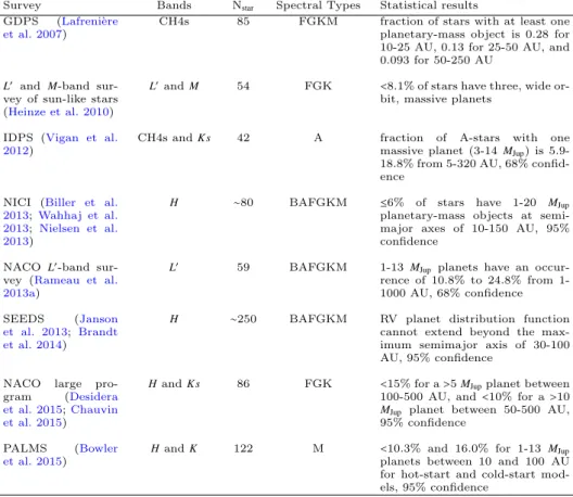
Coadding the frames in a data cube is a common practice but the best number of frames to coadd has not yet been thoroughly studied. We experimented with different numbers of coadded frames using fake planets. We ran the data through our PCA pipeline (detailed in Section 2.4.2) with different numbers of frames coadded (Figure 2.2). For example, 100 frames coadded means that twice as many images are passed to our pipeline as in the 200 coadded frames case. Figure 2.2

shows four S/N curves for planets injected a different angular separations, each with a S/N of approximately 10. The curves are offset from 10 for clarity. Coadding 200 or less frames yields a higher S/N. However, the S/N varies by less than a factor of two over all coadds, making this a relatively small effect. For the following analysis, we keep the coadds fixed at 200 frames, which yields S/N as good as less coadds, but is computationally much faster. This corresponds to∼70 coadded images in each hemisphere which are passed to our pipeline. Since there is little field rotation between individual frames in a data cube, the smearing effect within a cube is negligible.

2.4.1 LOCI

Locally optimized combination of images (Lafreni`ere et al. 2007) is a widely used planet detection algorithm which spatially models the stellar PSF to remove speckles. An image is divided into rings, which are subdivided into wedges. An optimal, lin-ear combination of images subtracts speckles within that region. The least squares fit succeeds at minimizing speckles, but also reduces the planet flux through the subtraction for small angular separations.

Each hemisphere dataset is processed with LOCI independently and the final three hemisphere sky aligned cubes are collapsed. Since we are using the APP, we only perform LOCI on the “dark side” of the image frames. This 180◦ D shaped region (inner=2λ/D, outer=7λ/D) is the only part of each frame that is coadded in the final image.

Kenworthy et al.(2013) analysis of these data used the LOCI algorithm. Monte Carlo simulations exploring LOCI parameters ensured that this is the best sensit-ivity LOCI could produce.

2.4.2 Principal Component Analysis

Principal component analysis is a mathematical technique that relies on the as-sumption that every image in a stack can be represented as a linear combination of its principal orthogonal components, selecting structures that are present in most of the images. Its recent application to high contrast exoplanet imaging (Amara & Quanz 2012;Soummer et al. 2012) has been shown to be very effective. Unlike LOCI (Lafreni`ere et al. 2007) which models the local stellar PSF structure, PCA models the global PSF structure.

(36)

7 8 9 10 11 12 13 14 15 S/N

0 10 20 30 40 50 60

0.0 0.2 0.4 0.6 0.8 1.0

Planet at 1.0" _{Flux ratio}

S/N 6 8 10 12 14 16 18 S/N

0 10 20 30 40 50 60

0.0 0.2 0.4 0.6 0.8 1.0

Flux Ratio (PCA Processed / Input)

Planet at 0.5"

5 6 7 8 9 10 11 12 13 14 S/N

0 10 20 30 40 50 60

# of PCs 0.0 0.2 0.4 0.6 0.8 1.0

Planet at 0.3"

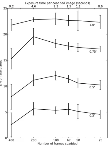
Figure 2.3 Comparison of the flux ratio and S/N based on number of PCs at different radii. The top panel is for a fake planet at 100.0, the middle panel is for

000.5 and the bottom panel is for 000.3. These panels demonstrate that, while the flux ratio does decrease with PCs, the S/N follows a different curve.

The number of PCs used determines how well the stellar PSF is fit. The first few components are the most stable, have less noise, and contain the most common structure in all the images. For our default analysis, we used 20 PCs to model the stellar PSF. PCA is run on each hemisphere dataset independently, as the PCs are correlated with time. The final de-rotated frames are coadded into one final image covering the full 360◦_{around the star.}

The following subsections discuss self-subtraction due to the PCA algorithm as well as a series of modifications we performed on PCA to optimize the detection of a planet at smallλ/D.

Self-subtraction

Self-subtraction from the LOCI algorithm has been well documented by previous authors (Lafreni`ere et al. 2007;Marois et al. 2010), but its impact on PCA is not yet well studied. The LOCI algorithm requires that the frames nearest in time to the current frame are not considered in the least squares fit, thus limiting the self-subtraction of a potential planet. However, this frame rejection technique does not completely account for flux loss from a planet.

(37)

0.5"

Figure 2.4 Image demonstrating the APP airy diffraction pattern with the radius limited region outlined in blue. This is the only region that is used in the data reduction.

background noise. In this paper, we address simply the detection mode.

Figure 2.3 shows three plots with the flux ratio and S/N versus the number of PCs it was processed with. The top figure is for a planet injected at 100.0, middle is at000.5and bottom is at000.3. The “flux ratio” is the ratio of the injected planet flux to the PCA processed flux in a 4 pixel aperture. For each angular separation, the L0 contrast which yields a S/N of approximately 10 is plotted. This figure demonstrates that the PCA method is more efficient at capturing the patterns associated with the background fluctuations of the field than capturing information associated with the planet translation. This differential effect means that in detection mode, it is acceptable for the flux ratio to decrease as long as the noise is decreasing as or more rapidly.

PCA Modifications

1. Frame Rejection

(38)

0 10 20 30 40 50 60 70 # of principal components

102

103

104

105

106

V

alu

e

of

ea

ch

c

oe

fficie

nt

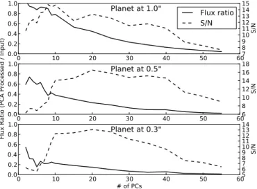
Figure 2.5 Plot of the PCA coefficient values. The highest PCA coefficient value corresponds to the most significant PC.

would appear to rotate faster between frames, thus less frames need to be rejected. This test allows us to compare the S/N of a fake planet processed with standard PCA and “0.5 FWHM rejection”, where we mimic the routine in LOCI to reject the frames closest in time.

2. Radius Limited

Next, we modified the PCA basis set by only using the image out to a certain radius. The outer radius (Rout) passed to the PCA code determines the amount of information provided to the SVD algorithm. Extra information does not ne-cessarily provide a better fit. Our previous applications of PCA keptRout fixed. The information passed to the SVD algorithm should be directly related to the stellar PSF. We modified our PCA code to varyRout based on the location of the fake planet. The new Rout is 1 λ/D greater than the radius of the fake planet (seeFigure 2.4), thus performing PCA on a smaller region. This experiment was performed to test how significant the stellar PSF fit was affected by radii greater than the planet location.

3. Number of PCs

The main parameter which can be manipulated in PCA is the number of PCs used in the SVD fit. The first principal value (the highest singular value in the diagonal matrix) is the “variance” of the image stack from the mean, in the direction of the first PC. The same is true about the second principal value and so on.

(39)

0.2 0.3 0.4 0.5 0.6 0.7 0.8 0.9 1.0 Radius [arcsec]

7

8

9

10

11

12

7 si

gm

a c

on

tra

st

NB4

.05

[m

ag

] 6

5

3 ₅

10

7 7 5

LOCI

PCA

PCA 0.5 FWHM rejection

PCA radius limited

PCA different # of PCs

Figure 2.6 Contrast curves for a 7σdetection of a point source in our Fomalhaut APP data processed with LOCI, ADI, and variations of ADI. The LOCI curve is adapted from Kenworthy et al.(2013) to a 7σ detection. The numbers on the yellow curve signify the number of PCs which yield the highest S/N at that radius. The dashed line is the background limit. The PCA contrast curves are the mean value for fake planets inserted at two P.A.s on opposite sides of the star (P.A.=45◦

and 225◦).

later values, implying that those PCs contain the most dominant features. Increas-ing the number of PCs in the stellar PSF fit can help brIncreas-ing out the planet signal by removing structure, however it also can add noise. Determining the optimal number of PCs for a certain stellar PSF fit is an essential but expensive task. The optimal number of PCs depends on the time variability of complex speckles. For each dataset and fake planet angular separation, PCA was run with different numbers of PCs ranging from 5 to 60, in increments of 5.

2.5 Results and Discussion

Figure 2.6shows the results of each image processing method detailed in Section

2.4.2. Each technique was run with varying planet contrasts at a given radius. We extrapolated between planet contrasts to determine contrast that yields a S/N of 7. For the method with varying PCs detailed in Section 2.4.2, we noted which number of PCs yielded the highest S/N at which radius. These are the numbers listed on the yellow curve inFigure 2.6.

(40)

Radiu s ("

) 0.2 0.3 0.4 0.5 0.6 0.7 0.8 0.9 1.0

# of principal compon_ents

10 ₂₀ 30 ₄₀ 50 C o n tr a s t (m a g ) 12 10 8 6 4 2 0

Figure 2.7 Three-dimensional surface of the contrast achieved in a 7σ detection with varied numbers of PCs. Varying the number of PCs at small angular separ-ations affects the 7σdetection limit by up to 8 mag. Beyond000.₆_{, the number of}

PCs used is less significant.

Unlike the LOCI algorithm, rejecting the frames nearest in time (detailed in Section2.4.2) yields a worse contrast curve than our standard PCA. This is likely due to the noise being more correlated in frames closer in time, thus providing important information to the SVD algorithm and increasing the S/N of the planet. We did not reject any frames in our final data analysis approach.

Limiting the outer radius passed to the SVD algorithm yielded a slightly better contrast ratio than standard PCA from000.5to000.8. However, this contrast increase is not significant and is only beneficial because it is less computationally expensive. Our standard PCA contrast curve was generated with 20 PCs. By varying the number of PCs we can increase the S/N from a companion. Our PC-varying result yields a consistently more sensitive contrast curve then all the other methods. We gain between 0.5 and 1 mag contrast over our LOCI analysis from 000.2 to 100.0. FromFigure 2.6we see that the number of PCs which yield the highest S/N for a planet varies based on its angular separation.

(41)

1 2 3 4 5 6 7 8 Radius [AU]

0 5 10 15 20 25 30 35 40

Jup

ite

r m

asse

s

PCA, Baraffe

PCA, Spiegel and Burrows

LOCI, Baraffe

LOCI, Spiegel and Burrows

0.2 0.3 0.4 0.5Radius [arcsec]0.6 0.7 0.8 0.9 1.0

Figure 2.8 Detection limit for fake companions around Fomalhaut generated with PCA (black lines) and LOCI (blue lines, converted to 7σdetection fromKenworthy et al. 2013) using (Baraffe et al. 2003, solid lines) and (Spiegel & Burrows 2012, dashed lines).

This can be seen inFigure 2.7as a contrast of nearly zero. As we move to larger radii the optimal number of PCs remains in the 5–20 PC range. Beyond000.6where the number of PCs shows no significant preference below 45 PCs.

2.5.1 Comparison with Kenworthy et al. (2013)

Our PCA re-analysis of these data improves sensitivity at small inner working angles, from000.2 to 1”, in some cases by 1 mag (see blue and yellow curves, Fig-ure 2.6). We convert the best 7σdetection contrast curve to an upper mass limit for planets using the Baraffe et al. (2003) and Spiegel & Burrows (2012) atmo-spheric models (Figure 2.8) assuming an age of 440 Myr (Mamajek et al. 2012). We confirm the non-detection of companions with a model-dependent upper mass limit of 13–18 MJup from 4–10 AU. Our new upper mass limit is based on our more robust 7σ detection limit. The 1 mag increase in the contrast ratio at 000.5

translates to an increased sensitivity of∆7MJup. The increase in sensitivity allows us to probe planetary masses (<15 MJup) at small angular separations.

Extrasolar planet detection through spatially resolved observations

The handle http://hdl.handle.net/1887/33272 holds various files of this Leiden University

dissertation.

Author: Meshkat, Tiffany

Through Spatially Resolved Observations

Proefschrift

Table of Contents

Chapter

1

Introduction

1.1

Directly Imaging Exoplanets

Radial Velocity

Transits

Microlensing

Direct Imaging

1.2

Planet Formation

1.3

Planet-Disk Interactions

1.4

Observing Strategies and Image Processing

1.4.1

Optical Aberrations

1.4.2

Adaptive optics

1.4.3

Coronagraphs

1.4.4

Angular Differential imaging

1.4.5

SDI

1.4.6

Locally optimized combination of images

1.4.7

Principal Component Analysis

1.5

Overview of Direct Imaging Surveys

1.6

This Thesis

References

Chapter

2

Optimized Principal Component

Analysis on Coronagraphic

Images of the Fomalhaut System

2.1

Introduction

2.2

Data

2.3

Creating the Simulated Data–Sets

2.4

Data Analysis

400

200

100

67 50

25

Number of frames coadded

0

5

10

15

20

25

S/N

of

fa

ke

pl

an

et

9.2

Exposure time per coadded image (seconds)

4.6

2.3

1.5 1.2

0.6

1.0"