Virtual water trade
A quantification of virtual
water flows between
nations in relation to
international crop trade
Value of Water
A.Y. Hoekstra
P.Q. Hung
September 2002
V
IRTUAL WATER TRADE
A
QUANTIFICATION OF VIRTUAL
WATER FLOWS BETWEEN NATIONS
IN RELATION TO INTERNATIONAL
CROP TRADE
A.Y. H
OEKSTRA
P.Q. H
UNG
S
EPTEMBER
2002
V
ALUE OF
W
ATER
R
ESEARCH
R
EPORT
S
ERIES
N
O
. 11
IHE D
ELFT
Contact author:
P.O. B
OX
3015
A.Y. Hoekstra
2601 DA D
ELFT
Tel. +31 15 2151828
T
HE
N
ETHERLANDS
E-mail [email protected]
Contents
Summary ...7
1. Introduction ...9
1.1. The economics of water use...9
1.2. Virtual water trade...10
1.3. The objective of this study...11
2. Method... 13
2.1. Calculation of specific water demand per crop type ...13
2.2. Calculation of virtual water trade flows and the national virtual water trade balance...14
2.3. Calculation of a nation’s ‘water footprint’...15
2.4. Calculation of national water scarcity, water dependency and water self-sufficiency ...16
3. Data sources ... 19
4. Specific water demand per crop type per country... 23
5. Global trade in virtual water... 25
5.1. International trade in virtual water...25
5.1.1. Overview of international virtual water trade... 25
5.1.2. Virtual water trade balance per country... 28
5.1.3. International virtual water trade by product... 34
5.2. Inter-regional trade in virtual water...35
5.2.1. Inter-regional virtual water trade relations... 35
5.2.2. Virtual water trade balance per world region ... 40
5.2.3. Gross virtual water trade between countries within regions... 50
5.3. Intercontinental trade in virtual water...51
5.3.1. Intercontinental virtual water trade relations... 51
5.3.2. Virtual water trade balance per continent... 53
5.3.3. Gross virtual water trade between countries within continents... 54
6. Virtual water trade of nations in relation to national water needs and availability... 55
6.1. Water footprints, water scarcity, water self-sufficiency and water dependency of nations ...55
6.2. The relation between water scarcity and water dependency ...60
7. Concluding remarks ... 63
Appendices
I.
Crop water requirements (m
3/ha)
II.
Actual crop yields (ton/ha) in 1999
III.
Specific water demands (m
3/ton) in 1999
IV.
FAO guidelines on crop water requirements in mm [=10 m
3/ha]
Va.
Gross virtual water import per country for the years 1995-1999 (10
6m
3)
Vb.
Gross virtual water export per country for the years 1995-1999 (10
6m
3)
Vc.
Net virtual water import per country for the years 1995-1999 (10
6m
3)
VI.
Classification of countries into thirteen world regions
Summary
The water that is used in the production process of an agricultural or industrial product is called the 'virtual
water' contained in the product. A water-scarce country might wish to import products that require a lot of water
in their production intensive products) and export products or services that require less water
(water-extensive products). This implies net import of ‘virtual water’ (as opposed to import of real water, which is
generally too expensive) and will relieve the pressure on the nation’s own water resources. Until date little is
known on the actual volumes of virtual water trade flows between countries.
The objective of this study is to quantify the volumes of all virtual water trade flows between nations in the
period 1995-1999 and to put the virtual water trade balances of nations within the context of national water
needs and water availability. The study has been limited to the quantification of virtual water trade flows related
to international crop trade.
The basic approach has been to multiply international crop trade flows (ton/yr) by their associated virtual water
content (m
3/ton). The required crop trade data have been taken from the United Nations Statistics Division in
New York. The required data on virtual water content of crops originating from different countries have been
estimated on the basis of various FAO databases (CropWat, ClimWat, FAOSTAT).
The calculations show that the global volume of crop-related virtual water trade between nations was 695
Gm
3/yr in average over the period 1995-1999. For comparison: the total water use by crops in the world has
been estimated at 5400 Gm
3/yr (Rockström and Gordon, 2001). This means that 13% of the water used for crop
production in the world is not used for domestic consumption but for export (in virtual form). This is the global
percentage; the situation strongly varies between countries.
Considering the period 1995-1999, the countries with largest net virtual water export are: United States, Canada,
Thailand, Argentina, and India. The countries with largest net virtual water import in the same period are: Sri
Lanka, Japan, the Netherlands, the Republic of Korea, and China.
For each nation of the world a ‘water footprint’ has been calculated (a term chosen on the analogy of the
‘ecological footprint’). The water footprint, equal to the sum of the domestic water use and net virtual water
import, is proposed here as a measure of a nation’s actual appropriation of the global water resources. It gives a
more complete picture than if one looks at domestic water use only, as is being done until date. In addition to the
water footprint, indicators are proposed for a nation’s ‘water self-sufficiency’ and a nation’s ‘water
dependency’.
In studying global virtual water trade flows, it is recommended to start working on other products than crops as
well, for instance livestock products such as meat. Another next step is to start interpreting the data and to study
how governments can deliberately interfere in the current national virtual water trade balances in order to
achieve higher global water use efficiency.
1. Introduction
1.1. The economics of water use
Water should be considered an economic good. Ten years after the Dublin conference this sounds like a mantra
for water policy makers. The sentence is repeated again and again, conference after conference. It is suggested
that problems of water scarcity, water excess and deterioration of water quality would be solved if the resource
‘water’ were properly treated as an economic good. The logic is clear: clean fresh water is a scarce good and
thus should be treated economically. There is an urgent need to develop appropriate concepts and tools to do so.
In dealing with the available water resources in an economically efficient way, there are three different levels at
which decisions can be made and improvements be achieved. The first level is the user level, where price and
technology play a key role. This is the level where the ‘local water use efficiency’ can be increased by creating
awareness, charging prices based on full marginal cost and by stimulating water-saving technology. Second, at a
higher level, a choice has to be made on how to allocate the available water resources to the different sectors of
economy (including public health and the environment). Water is used for the production of several ‘goods’ and
‘services’. People allocate water to serve certain purposes, which generally implies that other, alternative
purposes are not served. Choices on the allocation of water can be more or less ‘efficient’, depending on the
value of water in its alternative uses. At this level we speak of ‘water allocation efficiency’. Water is a public
good, so water allocation at the country or catchment level is principally a governmental issue. The question is
here how all demands for water can best be met and where – in case of water shortage – supply should be
restricted.
Beyond ‘local water use efficiency’ and ‘water allocation efficiency’ there is a level at which one could talk
about ‘global water use efficiency’. It is a fact that some regions of the world are water-scarce and other regions
are water-abundant. It is also a fact that in some regions there is a low demand for water and in other regions a
high demand. Unfortunately there is no general positive relation between water demand and availability. Until
recently people have focussed very much on considering how to meet demand based on the available water
resources at national or river basin scale. The issue is then how to most efficiently allocate and use the available
water. There is no reason to restrict the analysis to that. In a protected economy, a nation will have to achieve its
development goals with its own resources. In an open economy, however, a nation can import products that are
produced from resources that are scarcely available within the country and export products that are produced
with resources that are abundantly available within the country. A water-scarce country can thus aim at
importing products that require a lot of water in their production (water-intensive products) and exporting
products or services that require less water (water-extensive products). This is called
import of virtual water
(as
opposed to import of real water, which is generally too expensive) and will relieve the pressure on the nation’s
own water resources. For water-abundant countries an argumentation can be made for
export of virtual water
.
Import of water-intensive products by some nations and export of these products by others includes what is
called ‘virtual water trade’ between nations.
In summary, the overall efficiency in the appropriation of the global water resources can be defined as the ‘sum’
of local water use efficiencies, meso-scale water allocation efficiencies and global water use efficiency. So far
most attention of scientists and politicians has gone to local water use efficiency. There is quite some knowledge
available and improvements have actually been achieved already. More efficient allocation of water as a means
to improved water management has got quite same attention as well, but if it comes to the implementation of
improved allocation schemes there is still a long way to go. At the global level, it is even more severe, since
basic data on virtual water trade and water dependency of nations are generally even lacking. This has been the
incentive for this study.
1.2. Virtual water trade
For the production of nearly all goods water is required. The water that is used in the production process of an
agricultural or industrial product is called the 'virtual water' contained in the product. For example, for
producing a kilogram of grain, grown under rain-fed and favourable climatic conditions, we need about one to
two cubic metres of water, that is 1000 to 2000 kg of water. For the same amount of grain, but growing in an
arid country, where the climatic conditions are not favourable (high temperature, high evapotranspiration) we
need up to 3000 to 5000 kg of water.
If one country exports a water-intensive product to another country, it exports water in virtual form. In this way
some countries support other countries in their water needs. For water-scarce countries it could be attractive to
achieve water security by importing water-intensive products instead of producing all water-demanding
products domestically. Reversibly, water-rich countries could profit from their abundance of water resources by
producing water-intensive products for export. Trade of real water between water-rich and water-poor regions is
generally impossible due to the large distances and associated costs, but trade in water-intensive products
(virtual water trade) is realistic. Virtual water trade between nations and even continents could thus be used as
an instrument to improve global water use efficiency and to achieve water security in water-poor regions of the
world.
World-wide both politicians and the general public increasingly show interest in the pros and cons of
‘globalisation’ of trade. This can be understood from the fact that increasing global trade implies increased
Local water use efficiency
Water allocation efficiency
Global water use efficiency
virtual water trade between water-scarce and
water-abundant regions
technology, water price, environmental
awareness of water user
interdependence of nations. The tension in the debate relates to the fact that the game of global competition is
played with rules that many see as unfair. Knowing that economically sound water pricing is poorly developed
in many regions of the world, this means that many products are put on the world market at a price that does not
properly include the cost of the water contained in the product. This leads to situations in which some regions in
fact subsidise export of scarce water.
1.3. The objective of this study
The objectives of this study are:
1.
To estimate the amount of water needed to produce crops in different countries of the world;
2.
To quantify the volume of virtual water trade flows between nations in the period 1995-1999;
3.
To put the virtual water trade balances of nations within the context of national water needs and water
availability.
This report is primarily meant as a data report. We do not pretend to give an in-depth interpretation of the
results. Besides, we limit ourselves to virtual water trade in relation to international crop trade, thus excluding
virtual water trade related to international trade of livestock products and industrial products.
2. Method
2.1. Calculation of specific water demand per crop type
Per crop type, average specific water demand has been calculated separately for each relevant nation on the
basis of FAO data on crop water requirements and crop yields:
[ ]
[ ]
[ ]
c
n
CY
c
n
CWR
c
n
SWD
,
,
,
=
(1)
Here,
SWD
denotes the specific water demand (m
3ton
-1) of crop
c
in country
n
,
CWR
the crop water
requirement (m
3ha
-1) and
CY
the crop yield (ton ha
-1).
The crop water requirement
CWR
(in m
3ha
-1) is calculated from the accumulated crop evapotranspiration
ET
c(in mm/day) over the complete growing period. The crop evapotranspiration
ET
cfollows from multiplying the
‘reference crop evapotranspiration’
ET
0with the crop coefficient
K
c:
0
ET
K
ET
c=
c×
(2)
The concept of ‘reference crop evapotranspiration’ was introduced by FAO to study the evaporative demand of
the atmosphere independently of crop type, crop development and management practices. The only factors
affecting
ET
0are climatic parameters. The reference crop evapotranspiration
ET
0is defined as the rate of
evapotranspiration from a hypothetical reference crop with an assumed crop height of 12 cm, a fixed crop
surface resistance of 70 s m
-1and an albedo of 0.23. This reference crop evapotranspiration closely resembles
the evapotranspiration from an extensive surface of green grass cover of uniform height, actively growing,
completely shading the ground and with adequate water (Smith
et al.
, 1992). Reference crop evapotranspiration
is calculated on the basis of the FAO Penman-Monteith equation (Smith
et al
., 1992; Allen
et al
., 1994a, 1994b;
Allen
et al
., 1998):
)
34
.
0
1
(
)
(
273
900
)
(
408
.
0
2 2 0
U
e
e
U
T
G
R
ET
n a d+
+
∆
−
+
+
−
∆
=
γ
γ
(3)
in which:
ET
0= reference crop evapotranspiration [mm day
-1];
R
n= net radiation at the crop surface [MJ m
-2day
-1];
G
= soil heat flux [MJ m
-2day
-1];
T
= average air temperature [°C];
U
2= wind speed measured at 2 m height [m s
-1];
e
d= actual vapour pressure [kPa];
e
a-e
d= vapour pressure deficit [kPa];
∆
= slope of the vapour pressure curve [kPa °C
-1];
γ
= psychrometric constant [kPa °C
-1].
The crop coefficient accounts for the actual crop canopy and aerodynamic resistance relative to the hypothetical
reference crop. The crop coefficient serves as an aggregation of the physical and physiological differences
between a certain crop and the reference crop.
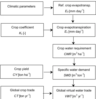
The overall scheme for the calculation of specific water demand is drawn in Figure 1.1. This figure also shows
the next step: the calculation of the virtual water trade flows between nations.
Figure 1.1. Steps in the calculation of global virtual water trade.
2.2. Calculation of virtual water trade flows and the national virtual water trade balance
Virtual water trade flows between nations have been calculated by multiplying international crop trade flows by
their associated virtual water content. The latter depends on the specific water demand of the crop in the
exporting country where the crop is produced. Virtual water trade is thus calculated as:
[
n
n
c
t
]
CT
[
n
n
c
t
]
SWD
[ ]
n
c
VWT
e,
i,
,
=
e,
i,
,
×
e,
(4)
Crop evapotranspiration
E
c[mm day
-1]
Crop water requirement
CWR
[m
3ha
-1]
Crop yield
CY
[ton ha
-1]
Specific water demand
SWD
[m
3ton
-1]
Global crop trade
CT
[ton yr
-1]
Global virtual water trade
VWT
[m
3yr
-1]
Ref. crop evapotransp.
E
0[mm day
-1]
Crop coefficient
K
c[-]
in which
VWT
denotes the virtual water trade (m
3yr
-1) from exporting country
n
eto importing country
n
iin year
t
as a result of trade in crop
c
.
C T
represents the crop trade (ton yr
-1) from exporting country
n
eto importing
country
n
iin year
t
for crop
c
.
SWD
represents the specific water demand (m
3ton
-1) of crop
c
in the exporting
country. Above equation assumes that if a certain crop is exported from a certain country, this crop is actually
grown in this country (and not in another country from which the crop was just imported for further export).
Although a certain error will be made in this way, it is estimated that this error will not substantially influence
the overall virtual water trade balance of a country. Besides, it is practically impossible to track the sources of
all exported products.
The gross virtual water import to a country
n
iis the sum of all imports:
[
]
∑
=
c n
i e i
e
t
c
n
n
VWT
t
n
GVWI
,
,
,
,
]
,
[
(5)
The gross virtual water export from a country
n
eis the sum of all exports:
[
]
∑
=
c n
i e e
i
t
c
n
n
VWT
t
n
GVWE
,
,
,
,
]
,
[
(6)
The net virtual water import of a country is equal to the gross virtual water import minus the gross virtual water
export. The virtual water trade balance of country
x
for year
t
can thus be written as:
[ ]
x
t
GVWI
[ ]
x
t
GVWE
[ ]
x
t
NVWI
,
=
,
−
,
(7)
where
NVWI
stands for the net virtual water import (m
3yr
-1) to the country. Net virtual water import to a
country has either a positive or a negative sign. The latter indicates that there is net virtual water
export
from the
country.
2.3. Calculation of a nation’s ‘water footprint’
The total water use within a country itself is not the right measure of a nation’s actual appropriation of the
global water resources. In the case of net import of virtual water import into a country, this virtual water volume
should be added to the total domestic water use in order to get a picture of a nation’s real call on the global
water resources. Similarly, in the case of net export of virtual water from a country, this virtual water volume
should be subtracted from the volume of domestic water use. The sum of domestic water use and net virtual
water import can be seen as a kind of ‘water footprint’ of a country, on the analogy of the ‘ecological footprint’
of a nation. In simplified terms, the latter refers to the amount of land needed for the production of the goods
and services consumed by the inhabitants of a country. Studies have shown that for some countries the
ecological footprint is smaller than the area of the nation’s territory, but in other cases much bigger
(Wackernagel and Rees, 1996; Wackernagel
et al
., 1997). The latter means that apparently some nations need
land outside their own territory to provide in their goods and services.
The ‘water footprint’ of a country (expressed as a volume of water per year) is defined as:
Water footprint
=
WU
+
NVWI
(8)
in which
WU
denotes the total domestic water use (m
3yr
-1) and
NVWI
the net virtual water import of a country
(m
3yr
-1). As noted earlier, the latter can have a negative sign as well.
Total domestic water use
WU
should ideally refer to the sum of ‘blue’ water use (referring to the use of
ground-and surface water) ground-and ‘green’ water use (referring to the use of precipitation). However, since data on green
water use on country basis are not easily obtainable, we have provisionally chosen in this report to limit the
definition of water use to blue water use. It should be noted that ‘net virtual water import’ as defined in the
previous section includes both ‘blue’ and ‘green’ water.
2.4. Calculation of national water scarcity, water dependency and water self-sufficiency
At the start of this study we expected to find a relation between national water scarcity and net virtual water
import. One would logically assume that a country with high water scarcity would seek to profit from net virtual
water import. On the other hand, countries with abundant water resources could make profit by exporting water
in virtual form. In order to check this hypothesis we need indices of both water scarcity and virtual water import
dependency. Plotting countries in a graph with water scarcity on the x-axis and virtual water import dependency
on the y-axis, would expectedly result in some positive relation.
As an index of national water scarcity we use the ratio of total water use to water availability:
100
×
=
WA
WU
WS
(9)
In this equation,
WS
denotes national water scarcity (%),
WU
the total water use in the country (m
3yr
-1) and
WA
the national water availability (m
3yr
-1). Defined in this way, water scarcity will generally range between zero
and hundred per cent, but can in exceptional cases (e.g. groundwater mining) be above hundred per cent. As a
measure of the national water availability
WA
we take the annual internal renewable water resources, that are the
average fresh water resources renewably available over a year from precipitation falling within a country’s
borders (see for instance Gleick, 1993). As noted in the previous section, total water use
WU
should ideally refer
to the sum of blue and green water use, but for practical reasons we have provisionally chosen in this report to
define water scarcity as the ratio of blue water use to water availability, which is generally done by others as
well.
Next, we have looked for a proper indicator of ‘virtual water import dependency’ or ‘water dependency’ in
brief. The indicator should reflect the level to which a nation relies on foreign water resources (through import
of water in virtual form). The water dependency
WD
of a nation is in this report calculated as the ratio of the net
virtual water import into a country to the total national water appropriation:
<
≥
×
+
=
0
if
0
0
if
100
NVWI
NVWI
NVWI
WU
NVWI
WD
(10)
The value of the water dependency index will per definition vary between zero and hundred per cent. A value of
zero means that gross virtual water import and export are in balance or that there is net virtual water export. If
on the other extreme the water dependency of a nation approaches hundred percent, the nation nearly completely
relies on virtual water import.
As the counterpart of the water dependency index, the water self-sufficiency index is defined as follows:
<
≥
×
+
=
0
if
100
0
if
100
NVWI
NVWI
NVWI
WU
WU
WSS
(11)
The water self-sufficiency of a nation relates to the water dependency of a nation in the following simple way:
WD
WSS
=
1
−
(12)
The level of water self-sufficiency
WSS
denotes the national capability of supplying the water needed for the
production of the domestic demand for goods and services. Self-sufficiency is hundred per cent if all the water
needed is available and indeed taken from within the own territory. Water self-sufficiently approaches zero if a
country heavily relies on virtual water imports.
3. Data sources
Data on crop water requirements are calculated with FAO’s CropWat model for Windows, which is available
through the web site of FAO (www.fao.org). The CropWat model uses the FAO Penman-Monteith equation for
calculating reference crop evapotranspiration as described in the previous chapter (Clarke
et al
., 1998). The
CropWat model calculates crop water requirement of different crop types on the basis of the following
assumptions:
(1) Crops are planted under optimum soil water conditions without any effective rainfall during their life; the
crop is developed under irrigation conditions.
(2) Crop evapotranspiration under standard conditions (ET
c), this is the evapotranspiration from disease-free,
well-fertilised crops, grown in large fields with 100% coverage.
(3) Crop coefficients are selected depending on the single crop coefficient approach, that means single
cropping pattern, not dual or triple cropping pattern.
Climatic data
The climatic data needed as input to CropWat have been taken from FAO’s climatic database ClimWat, which
is also available through FAO’s web site. The ClimWat database contains climatic data for more than hundred
countries. For many countries climatic data are available for different climatic stations. As a crude approach, the
capital climatic station data have been taken as the country representative. For the countries, where the required
climatic input data are not available in ClimWat, the crop water requirement is taken from the guideline of FAO
as reported by Gleick (1993) (Appendix IV). Depending on the country, the authors made an estimate
somewhere between the minimum and maximum estimate given in the FAO guideline. If still data were lacking,
data were taken from a neighbouring country.
Crop parameters
In the crop directory of the CropWat package sets of crop parameters are available for 24 different crops (Table
3.1). The crop parameters used as input data to CropWat are: the crop coefficients in different crop development
stages (initial, middle and late stage), the length of each crop in each development stage, the root depth, and the
planting date. For the 14 crops where crop parameters are not available in the CropWat package, crop
parameters have been based on Allen
et al
. (1998).
Crop yields
Table 3.1. Availability of crop parameters
.
Crops for which crop parameters have been taken from FAO’s
CropWat package
Crops for which crop parameters have been
taken from Allen
et al.
(1998)
Banana
Maize
Sugar beet
Artichoke
Onion dry
Barley
Mango
Sugar cane
Carrots
Peas
Bean dry
Millet
Sunflower
Cauliflower
Rice
Bean green
Oil palm fruit
Tobacco
Citrus
Safflower
Cabbage
Pepper
Tomato
Cucumber
Spinach
Cotton seeds
Potato
Vegetable
Lettuce
Sweet potato
Grape
Sorghum
Watermelon
Oats
Groundnut
Soybean
Wheat
Onion green
Global trade in crops
As a source for the global trade in crops, we have used the 1995-1999 data contained in the Personal Computer
Trade Analysis System (PC-TAS), a cd-rom produced by the United Nations Statistics Division (UNSD) in New
York in collaboration with the International Trade Centre (ITC) in Geneva. These data are based on the
Commodity Trade Statistics Data Base (COMTRADE) of the UNSD. Every year individual countries supply the
UNSD with their annual international trade statistics, detailed by commodity and partner country. These data are
processed into a standard format with consistent coding and valuation. Commodities are classified according the
Harmonised System (HS) classification of the World Customs Organization.
Link between two crop classifications
Specific water demand is calculated for 38 crop types as distinguished by the FAO in CropWat. The
Harmonised System (HS) classification used in the COMTRADE database is a much more detailed
classification. For our purpose we therefore have to link the two classifications, which has been done as shown
in Table 3.2.
Table 3.2. The link between FAO’s crop types and the Harmonised System classification.
FAO crop types
Commodities in the Harmonised System classification
Artichoke
Global artichoke, fresh or chilled
Banana
Banana, including plantains
Barley
Barley
Bean dried
Bean dry
Bean, small red, dried
Bean, frozen
Bean green
Bean, shelled or unshelled, fresh or chilled
Cabbage lettuce, fresh or chilled
Cabbage
Cabbages, konrabi
Carrots
Carrot, fresh or chilled
Cauliflower
Cauliflower and headed broccoli, fresh or chilled
Citrus fruit, fresh or dried
Citrus
FAO crop types
Commodities in the Harmonised System classification
Cotton seeds
Cotton seed, whether or not broken
Cucumber and gherkins provisionally preserved but not immediately consumption
Cucumber
Cucumber and gherkins, fresh or chilled
Sorghum
Grain sorghum
Grape dried
Grape
Grape fresh
Groundnut in shell whether or not broken
Groundnut
Groundnuts in shell or roasted
Lettuce
Lettuce, fresh or chilled
Maize
Maize (corn)
Millet
Millet
Oats
Oats
Onion dry
Onion dried, but not further prepared
Onion and shallots, fresh or chilled
Onion green
Onion, provisionally preserved
Oil palm fruit
Palm nut
Peas, dried, shelled
Peas, frozen
Peas
Peas, shelled or unshelled, fresh or chilled
Pepper
Pepper of the genius capsuis
Potato, fresh or chilled
Potato
Potatoes, frozen
Sugar beet
Raw sugar beet
Sugar cane
Raw sugar can
Rice, broken
Rice, husked, (brown)
Rice
Rice, in the husk (paddy or rough)
Safflower
Safflower seed, whether or not broken
Soybean
Soybean
Spinach
Spinach, N-Z spinach orache spinach
Sunflower
Sunflower seed
Sweet potato
Sweet potatoes, fresh or dried
Tobacco, unmanufactured, not stemmed
Tobacco
Tobacco, unmanufactured, partly or wholly stemmed
Tomato
Tomatoes, fresh or chilled
Vegetable, fresh or chilled
Vegetable
vegetable, frozen
Wheat
Durum wheat
Wheat
4. Specific water demand per crop type per country
The calculated crop water requirements for different crops in different countries are shown in Appendix I. The
crop water requirements as calculated here refer to the evapotranspiration under optimal growth conditions (see
Chapter 3). This means that the calculated values are overestimates, because in reality there are often water
shortage conditions. On the other hand, the calculated values can also be seen as conservative, because they
exclude inevitable losses (e.g. during transport and application of water) and required losses such as drainage.
The calculated crop water requirements differ considerably over countries, which is mainly due to the
differences in climatic conditions.
Data on actual crop yields in the year 1999 have been retrieved from the FAOSTAT database. The data, which
are country averages, are shown in Appendix II. Where country specific crop yield data are lacking in
FAOSTAT, regional averages have been taken. The values that have been assessed in this way are presented in
grey-shadow cells in Appendix II. The differences between countries are here even larger than in the case of the
crop water requirements. This is due to the impact of the human factor on the actual crop yields.
Specific water demand (m
3/ton) per crop type has been calculated for different countries by dividing the crop
water requirement (m
3/ha) by the crop yield (ton/ha). The results are shown in Appendix III. Because both crop
water requirements and crop yields strongly vary between countries, specific water demands vary as well.
It is noted here that the specific water demand data for 1999 will be used to calculate the virtual water trade
flows in the whole period 1995-1999 (see Chapter 5). This is acceptable because country crop yield data appear
not to vary considerably over years.
5. Global trade in virtual water
5.1. International trade in virtual water
5.1.1. Overview of international virtual water trade
The calculation results show that the global volume of crop-related virtual water trade between nations was 695
Gm
3/yr in average over the period 1995-1999. For comparison: the global water withdrawal for agriculture
(water use for irrigation) was about 2500 Gm
3/yr in 1995 and 2600 Gm
3/yr in 2000 (Shiklomanov, 1997, p.61).
Taking into account the use of rainwater by crops as well, the total water use by crops in the world has been
estimated at 5400 Gm
3/yr (Rockström and Gordon, 2001, p.847). This means that 13% of the water used for
crop production in the world is not used for domestic consumption but for export (in virtual form). This is the
global percentage; the situation strongly varies between countries.
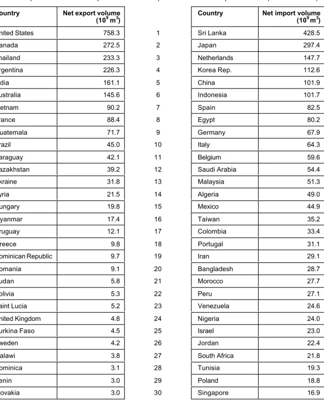
Considering the period 1995-1999, the top-5 list of countries with net virtual water export is: 1st. United States,
2nd. Canada, 3rd. Thailand, 4th. Argentina, and 5th. India. The top-5 list of countries in terms of net virtual
water import for the same period is: 1st. Sri Lanka, 2nd. Japan, 3rd. Netherlands, 4th. Republic of Korea, and
5th. China. Top-30 lists are given in Table 5.1. The ranking lists do not considerably change if we look into
particular years within the five-year period 1995-1999.
Figure 5.1. National virtual water trade balances over the period 1995-1999.
Green coloured countries have net virtual water export. Red coloured countries have net virtual water import.
Net virtual water import, Gm3
-100- -800 -10- -100 -1- -10
0- -1 0- 1 1- 10 10- 50 50- 100 100- 500