Sublinear-time algorithms
∗
Artur Czumaj
†Christian Sohler
‡Abstract
In this paper we survey recent advances in the area of sublinear-time algorithms.
1
Introduction
T
He area of sublinear-time algorithms is a new rapidly emerging area of computer science. Ithas its roots in the study of massive data sets that occur more and more frequently in var-ious applications. Financial transactions with billions of input data and Internet traffic analyses (Internet traffic logs, clickstreams, web data) are examples of modern data sets that show unprece-dented scale. Managing and analyzing such data sets forces us to reconsider the traditional notions of efficient algorithms: processing such massive data sets in more than linear time is by far too expensive and often even linear time algorithms may be too slow. Hence, there is the desire to
develop algorithms whose running times are not only polynomial, but in fact are sublinear inn.
Constructing a sublinear time algorithm may seem to be an impossible task since it allows one to read only a small fraction of the input. However, in recent years, we have seen development of sublinear time algorithms for optimization problems arising in such diverse areas as graph theory, geometry, algebraic computations, and computer graphics. Initially, the main research focus has been on designing efficient algorithms in the framework of property testing (for excellent surveys, see [26, 30, 31, 40, 49]), which is an alternative notion of approximation for decision problems. But more recently, we see some major progress in sublinear-time algorithms in the classical model of randomized and approximation algorithms. In this paper, we survey some of the recent advances in this area. Our main focus is on sublinear-time algorithms for combinatorial problems, especially for graph problems and optimization problems in metric spaces.
Our goal is to give a flavor of the area of sublinear-time algorithms. We focus on the most representative results in the area and we aim to illustrate main techniques used to design sublinear-time algorithms. Still, many of the details of the presented results are omitted and we recommend
∗Research supported in part by NSF ITR grant CCR-0313219 and NSF DMS grant 0354600.
†Department of Computer Science, New Jersey Institute of Technology and Department of Computer Science,
University of Warwick. Email: [email protected].
‡Department of Computer Science, Rutgers University and Heinz Nixdorf Institute, University of Paderborn.
the readers to follow the original works. We also do not aim to cover the entire area of sublinear-time algorithms, and in particular, we do not discuss property testing algorithms [26, 30, 31, 40, 49], even though this area is very closely related to the research presented in this survey.
Organization. We begin with an introduction to the area and then we give some sublinear-time algorithms for a basic problem in computational geometry [14]. Next, we present recent sublinear-time algorithms for basic graph problems: approximating the average degree in a graph [25, 34] and estimating the cost of a minimum spanning tree [15]. Then, we discuss sublinear-time algorithms for optimization problems in metric spaces. We present the main ideas behind recent algorithms for estimating the cost of minimum spanning tree [19] and facility location [10], and then we discuss the quality of random sampling to obtain sublinear-time algorithms for clustering problems [20, 46]. We finish with some conclusions.
2
Basic Sublinear Algorithms
The concept of sublinear-time algorithms is known for a very long time, but initially it has been used to denote “pseudo-sublinear-time” algorithms, where after an appropriate preprocessing, an
algorithm solves the problem in sublinear-time. For example, if we have a set ofnnumbers, then
after anO(nlogn)preprocessing (sorting), we can trivially solve a number of problems involving
the input elements. And so, if the after the preprocessing the elements are put in a sorted array,
then inO(1)time we can find the kth smallest element, inO(logn)time we can test if the input
contains a given elementx, and also inO(logn)time we can return the number of elements equal
to a given elementx. Even though all these results are folklore, this is not what we call nowadays
a sublinear-time algorithm.
In this survey, our goal is to study algorithms for which the input is taken to be in any standard representation and with no extra assumptions. Then, an algorithm does not have to read the entire input but it may determine the output by checking only a subset of the input elements. It is easy to see that for many natural problems it is impossible to give any reasonable answer if not all or almost all input elements are checked. But still, for some number of problems we can obtain good algorithms that do not have to look at the entire input. Typically, these algorithms are randomized (because most of the problems have a trivial linear-time deterministic lower bound) and they return only an approximate solution rather than the exact one (because usually, without looking at the whole input we cannot determine the exact solution). In this survey, we present recently developed sublinear-time algorithm for some combinatorial optimization problems.
Searching in a sorted list. It is well-known that if we can store the input in a sorted array, then we can solve various problems on the input very efficiently. However, the assumption that the input array is sorted is not natural in typical applications. Let us now consider a variant of this problem,
where our goal is to search for an elementxin a linked sorted list containingndistinct elements1.
1The assumption that the input elements are distinct is important. If we allow multiple elements to have the same
Here, we assume that thenelements are stored in a doubly-linked, each list element has access to
the next and preceding element in the list, and the list is sorted (that is, ifx followsy in the list,
theny < x). We also assume that we have access to all elements in the list, which for example,
can correspond to the situation that alln list elements are stored in an array (but the array is not
sorted and we do not impose any order for the array elements). How can we find whether a given
numberxis in our input or is not?
On the first glace, it seems that since we do not have direct access to the rank of any element
in the list, this problem requires Ω(n)time. And indeed, if our goal is to design a deterministic
algorithm, then it is impossible to do the search ino(n)time. However, if we allow randomization,
then we can complete the search inO(√n)expected time (and this bound is asymptotically tight).
Let us first sample uniformly at random a setS ofΘ(√n)elements from the input. Since we
have access to all elements in the list, we can select the setSinO(√n)time. Next, we scan all the
elements inS and in O(√n)time we can find two elements inS, pandq, such thatp ≤ x < q,
and there is no element in S that is between p and q. Observe that since the input consist of n
distinct numbers, pandqare uniquely defined. Next, we traverse the input list containing all the
input elements starting atpuntil we find either the sought keyxor we find elementq.
Lemma 1 The algorithm above completes the search in expected O(√n) time. Moreover, no algorithm can solve this problem ino(√n)expected time.
Proof. The running time of the algorithm if equal toO(√n)plus the number of the input elements
between p and q. Since S contains Θ(√n) elements, the expected number of input elements
between p and q is O(n/|S|) = O(√n). This implies that the expected running time of the
algorithm isO(√n).
For a proof of a lower bound ofΩ(√n)expected time, see, e.g., [14]. ⊓⊔
2.1
Geometry: Intersection of Two Polygons
Let us consider a related problem but this time in a geometric setting. Given two convex polygons
AandB inR2, each withnvertices, determine if they intersect, and if so, then find a point in their
intersection.
It is well known that this problem can be solved inO(n)time, for example, by observing that
it can be described as a linear programming instance in 2-dimensions, a problem which is known to have a linear-time algorithm (cf. [24]). In fact, within the same time one can either find a point
that is in the intersection ofA andB, or find a lineL that separatesAfromB (actually, one can
even find a bitangent separating lineL, i.e., a line separating AandB which intersects with each
ofAandB in exactly one point). The question is whether we can obtain a better running time.
The complexity of this problem depends on the input representation. In the most powerful model, if the vertices of both polygons are stored in an array in cyclic order, Chazelle and Dobkin [13] showed that the intersection of the polygons can be determined in logarithmic time. However,
a standard geometric representation assumes that the input is not stored in an array but rather A
andB are given by their doubly-linked lists of vertices such that each vertex has as its successor
the next vertex of the polygon in the clockwise order. Can we then test ifAandB intersect?
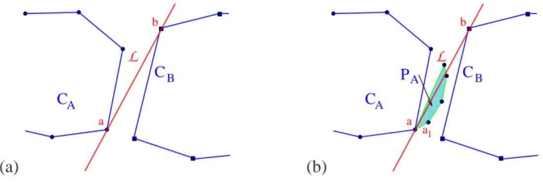
(a) C CB A a b L (b) 000000000 000000000 000000000 000000000 000000000 000000000 000000000 000000000 000000000 000000000 000000000 000000000 000000000 000000000 000000000 000000000 000000000 000000000 000000000 000000000 000000000 000000000 000000000 000000000 000000000 000000000 000000000 000000000 000000000 000000000 000000000 000000000 000000000 000000000 000000000 111111111 111111111 111111111 111111111 111111111 111111111 111111111 111111111 111111111 111111111 111111111 111111111 111111111 111111111 111111111 111111111 111111111 111111111 111111111 111111111 111111111 111111111 111111111 111111111 111111111 111111111 111111111 111111111 111111111 111111111 111111111 111111111 111111111 111111111 111111111 A C CA B b a a L P 1
Figure 1: (a) Bitangent lineLseparatingCAandCB, and (b) the polygonPA.
Chazelle et al. [14] gave anO(√n)-time algorithm that reuses the approach discussed above
for searching in a sorted list. Let us first sample uniformly at randomΘ(√n)vertices from each
AandB, and let CAandCB be the convex hulls of the sample point sets for the polygonsAand
B, respectively. Using the linear-time algorithm mentioned above, inO(√n)time we can check if
CAandCB intersects. If they do, then the algorithm will get us a point that lies in the intersection
ofCAandCB, and hence, this point lies also in the intersection ofAandB. Otherwise, let Lbe
the bitangent separating line returned by the algorithm (see Figure 1 (a)).
Leta andbbe the points in Lthat belong toAandB, respectively. Leta1 anda2 be the two
vertices adjacent toainA. We will define now a new polygonPA. If none ofa1 anda2 is on the
sideCAofLthe we definePAto be empty. Otherwise, exactly one ofa1 anda2 is on the sideCA
ofL; let it bea1. We define polygonPAby walking fromatoa1and then continue walking along
the boundary ofAuntil we cross Lagain (see Figure 1 (b)). In a similar way we define polygon
PB. Observe that the expected size of each ofPAandPB is at mostO(√n).
It is easy to see that Aand B intersects if and only if either A intersects PB orB intersects
PA. We only consider the case of checking ifAintersectsPB. We first determine ifCAintersects
PB. If yes, then we are done. Otherwise, letLAbe a bitangent separating line that separatesCA
fromPB. We use the same construction as above to determine a subpolygonQAofAthat lies on
thePB side ofLA. Then,AintersectsPB if and only ifQAintersectsPB. SinceQAhas expected
sizeO(√n)and so doesPB, testing the intersection of these two polygons can be done inO(√n)
expected time. Therefore, by our construction above, we have solved the problem of determining
if two polygons of size n intersect by reducing it to a constant number of problem instances of
determining if two polygons of expected sizeO(√n)intersect. This leads to the following lemma.
Lemma 2 [14] The problem of determining whether two convexn-gons intersect can be solved in
O(√n)expected time, which is asymptotically optimal.
Chazelle et al. [14] gave not only this result, but they also showed how to apply a similar approach to design a number of sublinear-time algorithms for some basic geometric problems. For example, one can extend the result discussed above to test the intersection of two convex polyhedra
inR3withnvertices inO(√n)expected time. One can also approximate the volume of ann-vertex
convex polytope to within a relative errorε >0in expected timeO(√n/ε). Or even, for a pair of
two points on the boundary of a convex polytopeP withnvertices, one can estimate the length of
an optimal shortest path outsideP between the given points inO(√n)expected time.
In all the results mentioned above, the input objects have been represented by a linked
struc-ture: either every point has access to its adjacent vertices in the polygon inR2, or the polytope is
defined by a doubly-connected edge list, or so. These input representations are standard in com-putational geometry, but a natural question is whether this is necessary to achieve sublinear-time algorithms — what can we do if the input polygon/polytop is represented by a set of points and no additional structure is provided to the algorithm? In such a scenario, it is easy to see that no
o(n)-time algorithm can solve exactly any of the problems discussed above. That is, for example,
to determine if two polygons withnvertices intersect one needsΩ(n)time. However, still, we can
obtain some approximation to this problem, one which is described in the framework of property
testing.
Suppose that we relax our task and instead of determining if two (convex) polytopesAandBin
Rdintersects, we just want to distinguish between two cases: eitherAandB are intersection-free,
or one has to “significantly modify” A and B to make them intersection-free. The definition of
the notion of “significantly modify” may depend on the application at hand, but the most natural
characterization would be to remove at leastε npoints inAandB, for an appropriate parameterε
(see [18] for a discussion about other geometric characterization). Czumaj et al. [23] gave a simple
algorithm that for anyε >0, can distinguish between the case whenAandB do not intersect, and
the case when at leastε npoints has to be removed fromAandB to make them intersection-free:
the algorithm returns the outcome of a test if a random sample ofO((d/ε) log(d/ε))points from
Aintersects with a random sample ofO((d/ε) log(d/ε))points fromB.
Sublinear-time algorithms: perspective. The algorithms presented in this section should give a flavor of the area and give us the first impression of what do we mean by sublinear-time and what kind of results one can expect. In the following sections, we will present more elaborate algorithms for various combinatorial problems for graphs and for metric spaces.
3
Sublinear Time Algorithms for Graphs Problems
In the previous section, we introduced the concept of sublinear-time algorithms and we presented two basic sublinear-time algorithms for geometric problems. In this section, we will discuss sublinear-time algorithms for graph problems. Our main focus is on sublinear-time algorithms for graphs, with special emphasizes on sparse graphs represented by adjacency lists where combi-natorial algorithms are sought.
3.1
Approximating the Average Degree
Assume we have access to the degree distribution of the vertices of an undirected connected graph
approximation of the average degree inG by looking at a sublinear number of vertices? At first sight, this seems to be an impossible task. It seems that approximating the average degree is
equivalent to approximating the average of a set ofn numbers with values between1andn−1,
which is not possible in sublinear time. However, Feige [25] proved that one can approximate the
average degree inO(√n/ε)time within a factor of2 +ε.
The difficulty with approximating the average of a set ofnnumbers can be illustrated with the
following example. Assume that almost all numbers in the input set are1and a few of them are
n−1. To approximate the average we need to approximate how many occurrences ofn−1exist.
If there is only a constant number of them, we can do this only by looking atΩ(n)numbers in the
set. So, the problem is that these large numbers can “hide” in the set and we cannot give a good approximation, unless we can “find” at least some of them.
Why is the problem less difficult, if, instead of an arbitrary set of numbers, we have a set of numbers that are the vertex degrees of a graph? For example, we could still have a few vertices of
degreen−1. The point is that in this case any edge incident to such a vertex can be seen at another
vertex. Thus, even if we do not sample a vertex with high degree we will see all incident edges at other vertices in the graph. Hence, vertices with a large degree cannot “hide.”
We will sketch a proof of a slightly weaker result than that originally proven by Feige [25].
Let d denote the average degree in G = (V, E) and let dS denote the random variable for the
average degree of a setS ofsvertices chosen uniformly at random from V. We will show that if
we sets≥β√n/εO(1)for an appropriate constantβ, thend
S ≥(12−ε)·dwith probability at least
1−ε/64. Additionally, we observe that Markov inequality immediately implies thatdS ≤(1+ε)·d
with probability at least1−1/(1 +ε)≥ε/2. Therefore, our algorithm will pick8/εsetsSi, each
of sizes, and output the set with the smallest average degree. Hence, the probability that all of
the sets Si have too high average degree is at most (1− ε/2)ε/8 ≤ 1/8. The probability that
one of them has too small average degree is at most 8ε · 64ε = 1/8. Hence, the output value will
satisfy both inequalities with probability at least 3/4. By replacing ε withε/2, this will yield a
(2 +ε)-approximation algorithm.
Now, our goal is to show that with high probability one does not underestimate the average
degree too much. LetHbe the set of the√ε nvertices with highest degree inGand letL=V \H
be the set of the remaining vertices. We first argue that the sum of the degrees of the vertices
in L is at least(1
2 −ε) times the sum of the degrees of all vertices. This can be easily seen by
distinguishing between edges incident to a vertex from Land edges withinH. Edges incident to
a vertex from L contribute with at least 1 to the sum of degrees of vertices in L, which is fine
as this is at least 1/2 of their full contribution. So the only edges that may cause problems are
edges withinH. However, since|H|=√ε n, there can be at mostε nsuch edges, which is small
compared to the overall number of edges (which is at leastn−1, since the graph is connected).
Now, let dH be the degree of a vertex with the smallest degree inH. Since we aim at giving a
lower bound on the average degree of the sampled vertices, we can safely assume that all sampled
vertices come from the setL. We know that each vertex inLhas a degree between1anddH. Let
from Hoeffding bounds that
Pr[ s X
i=1
Xi ≤(1−ε)·E[ s X
i=1
Xi]] ≤ e
−E[
Pr
i=1Xi]·ε2
dH .
We know that the average degree is at leastdH· |H|/n, because any vertex inHhas at least degree
dH. Hence, the average degree of a vertex inL is at least(12 −ε)·dH · |H|/n. This just means
E[Xi]≥(1
2−ε)·dH·|H|/n. By linearity of expectation we getE[
Ps
i=1Xi]≥s·(12−ε)·dH·|H|/n.
This implies that, for our choice ofs, with high probability we havedS ≥(12 −ε)·d.
Feige showed the following result, which is stronger with respect to the dependence onε.
Theorem 3 [25] UsingO(ε−1 ·pn/d
0)queries, one can estimate the average degree of a graph
within a ratio of(2 +ε), provided thatd≥d0.
Feige also proved thatΩ(ε−1·pn/d)queries are required, wheredis the average degree in the
input graph. Finally, any algorithm that uses only degree queries and estimates the average degree
within a ratio2−δfor some constantδrequiresΩ(n)queries.
Interestingly, if one can also use neighborhood queries, then it is possible to approximate the
average degree usingOe(√n/εO(1))queries with a ratio of(1 +ε), as shown by Goldreich and Ron
[34]. The model for neighborhood queries is as follows. We assume we are given a graph and we
can query for theith neighbor of vertexv. If v has at least ineighbors we get the corresponding
neighbor; otherwise we are told thatv has less thanineighbors. We remark that one can simulate
degree queries in this model withO(logn)queries. Therefore, the algorithm from [34] uses only
neighbor queries.
For a sketch of a proof, let us assume that we know the setH. Then we can use the following
approach. We only consider vertices fromL. If our sample contains a vertex fromH we ignore
it. By our analysis above, we know that there are only few edges withinHand that we make only
a small error in estimating the number of edges within L. We loose the factor of two, because
we “see” edges from Lto H only from one side. The idea behind the algorithm from [34] is to
approximate the fraction of edges fromLtoH and add it to the final estimate. This has the effect
that we count any edge betweenLandH twice, canceling the effect that we see it only from one
side. This is done as follows. For each vertexvwe sample fromLwe take a random set of incident
edges to estimate the fraction λ(v) of its neighbors that is in H. Let λˆ(v) denote the estimate
we obtain. Then our estimate for the average degree will bePv∈S∩L(1 + ˆλ(v))·d(v)/|S ∩L|,
whered(v)denotes the degree of v. If for all vertices we estimate λ(v)within an additive error
ofε, the overall error induced by theλˆ will be small. This can be achieved with high probability
queryingO(logn/ε2)random neighbors. Then the output value will be a(1 +ε)-approximation of
the average degree. The assumption that we knowH can be dropped by taking a set ofO(pn/ε)
vertices and setting H to be the set of vertices with larger degree than all vertices in this set
(breaking ties by the vertex number).
(We remark that the outline of a proof given above is different from the proof in [34].)
Theorem 4 [34] Given the ability to make neighbor queries to the input graphG, there exists an algorithm that makes O(pn/d0 ·ε−O(1)) queries and approximates the average degree inG to
3.2
Minimum Spanning Trees
One of the most fundamental graph problems is to compute a minimum spanning tree. Since the minimum spanning tree is of size linear in the number of vertices, no sublinear algorithm for sparse
graphs can exists. It is also know that no constant factor approximation algorithm witho(n2)query
complexity in dense graphs (even in metric spaces) exists [37]. Given these facts, it is somewhat surprising that it is possible to approximate the cost of a minimum spanning tree in sparse graphs
[15] as well as in metric spaces [19] to within a factor of(1 +ε).
In the following we will explain the algorithm for sparse graphs by Chazelle et al. [15]. We will
prove a slightly weaker result than in [15]. LetG = (V, E)be an undirected connected weighted
graph with maximum degree Dand integer edge weights from {1, . . . , W}. We assume that the
graph is given in adjacency list representation, i.e., for every vertexv there is a list of its at most
Dneighbors, which can be accessed fromv. Furthermore, we assume that the vertices are stored
in an array such that it is possible to select a vertex uniformly at random. We assume also that the
values ofDandW are known to the algorithm.
The main idea behind the algorithm is to express the cost of a minimum spanning tree as the
number of connected components in certain auxiliary subgraphs ofG. Then, one runs a
random-ized algorithm to estimate the number of connected components in each of these subgraphs.
To start with basic intuitions, let us assume that W = 2, i.e., the graph has only edges of
weight1or2. LetG(1) = (V, E(1))denote the subgraph that contains all edges of weight (at most)
1and letc(1) be the number of connected components inG(1). It is easy to see that the minimum
spanning tree has to link these connected components by edges of weight2. Since any connected
component in G(1) can be spanned by edges of weight 1, any minimum spanning tree ofG has
c(1)−1edges of weight2andn−1−(c(1)−1)edges of weight1. Thus, the weight of a minimum
spanning tree is
n−1−(c(1)−1) + 2·(c(1)−1) = n−2 +c(1) = n−W +c(1) .
Next, let us consider an arbitrary integer value forW. DefiningG(i)= (V, E(i)), whereE(i) is the
set of edges in Gwith weight at most i, one can generalize the formula above to obtain that the
costMST of a minimum spanning tree can be expressed as
MST = n−W +
WX−1
i=1
c(i) .
This gives the following simple algorithm.
APPROXMSTWEIGHT(G, ε)
fori= 1toW −1
Compute estimatorbc(i)forc(i)
outputMST] =n−W +PiW=1−1bc(i)
Thus, the key question that remains is how to estimate the number of connected components. This is done by the following algorithm.
APPROXCONNECTEDCOMPS(G, s) {Input: an arbitrary undirected graphG}
{Output:ˆc: an estimation of the number of connected components ofG}
choosesverticesu1, . . . , usuniformly at random
fori= 1tosdo
chooseX according toPr[X ≥k] = 1/k
run breadth-fist-search (BFS) starting atui until either
(1) the whole connected component containingui has been explored, or
(2)Xvertices have been explored
if BFS stopped in case (1) thenbi = 1 elsebi = 0
outputˆc= n s
Ps i=1bi
To analyze this algorithm let us fix an arbitrary connected componentC and let|C|denote the
number of vertices in the connected component. Letcdenote the number of connected components
inG. We can write
E[bi] = X
connected componentC
Pr[ui ∈C]·Pr[X ≥ |C|] = X
connected componentC
|C|
n ·
1
|C| = c n .
And by linearity of expectation we obtainE[ˆc] =c.
To show thatˆcis concentrated around its expectation, we apply Chebyshev inequality. Sincebi
is an indicator random variable, we have
Var[bi] = E[b2
i]−E[bi]2 ≤E[b2i] =E[bi] =c/n .
Thebiare mutually independent and so we have
Var[ˆc] = Varn s ·
s X
i=1
bi
= n
2
s2 ·
s X
i=1
Var[bi]≤ n·c
s .
With this bound forVar[ˆc], we can use Chebyshev inequality to obtain
Pr[|cˆ−E[cb]| ≥λn] ≤ n·c s·λ2·n2 ≤
1
λ2 ·s .
From this it follows that one can approximate the number of connected components within additive
error ofλnin a graph with maximum degreeDinO(Dλ·log2·̺n)time and with probability1−̺. The
following somewhat stronger result has been obtained in [15]. Notice that the obtained running
time is independent of the input sizen.
Theorem 5 [15] The number of connected components in a graph with maximum degreeDcan be approximated with additive error at most±λ ninO(D
Now, we can use this procedure with parameters λ = ε/(2W) and ̺ = 1
4W in algorithm
APPROXMSTWEIGHT. The probability that at least one call to APPROXCONNECTEDCOMPSis
not within an additive error ±λn is at most 1/4. The overall additive error is at most ±εn/2.
Since the cost of the minimum spanning tree is at leastn−1≥n/2, it follows that the algorithms
computes in O(D·W3 ·logn/ε2)time a(1±ε)-approximation of the weight of the minimum
spanning tree with probability at least3/4. In [15], Chazelle et al. proved a slightly stronger result
which has running time independent of the input size.
Theorem 6 [15] Algorithm APPROXMSTWEIGHTcomputes a valueMST] that with probability
at least3/4satisfies
(1−ε)·MST ≤ MST] ≤(1 +ε)·MST .
The algorithm runs inOe(D·W/ε2)time.
The same result also holds when D is only the average degree of the graph (rather than the
maximum degree) and the edge weights are reals from the interval [1, W] (rather than integers)
[15]. Observe that, in particular, for sparse graphs for which the ratio between the maximum and the minimum weight is constant, the algorithm from [15] runs in constant time!
It was also proved in [15] that any algorithm estimatingMST requiresΩ(D·W/ε2)time.
3.3
Other Sublinear-time Results for Graphs
In this section, our main focus was on combinatorial algorithms for sparse graphs. In particular, we did not discuss a large body of algorithms for dense graphs represented in the adjacency matrix model. Still, we mention the results of approximating the size of the maximum cut in constant time for dense graphs [28, 32], and the more general results about approximating all dense problems in Max-SNP in constant time [2, 8, 28]. Similarly, we also have to mention about the existence of a large body of property testing algorithms for graphs, which in many situations can lead to sublinear-time algorithms for graph problems. To give representative references, in addition to the excellent survey expositions [26, 30, 31, 40, 49], we want to mention the recent results on testability of graph properties, as described, e.g., in [3, 4, 5, 6, 11, 21, 33, 43].
4
Sublinear Time Approximation Algorithms for Problems in
Metric Spaces
One of the most widely considered models in the area of sublinear time approximation algorithms
is the distance oracle model for metric spaces. In this model, the input of an algorithm is a setP
ofnpoints in a metric space(P, d). We assume that it is possible to compute the distanced(p, q)
between any pair of pointsp, qin constant time. Equivalently, one could assume that the algorithm
matrix of a weighted undirected complete graph. Since the full description size of this matrix is
Θ(n2), we will call any algorithm witho(n2)running time a sublinear algorithm.
Which problems can and cannot be approximated in sublinear time in the distance oracle model? One of the most basic problems is to find (an approximation) of the shortest or the longest pairwise distance in the metric space. It turns out that the shortest distance cannot be approximated.
The counterexample is a uniform metric (all distances are1) with one distance being set to some
very small value ε. Obviously, it requires Ω(n2) time to find this single short distance. Hence,
no sublinear time approximation algorithm for the shortest distance problem exists. What about
the longest distance? In this case, there is a very simple 12-approximation algorithm, which was
first observed by Indyk [37]. The algorithm chooses an arbitrary point pand returns its furthest
neighborq. Letr, sbe the furthest pair in the metric space. We claim thatd(p, q)≥ 1
2d(r, s). By
the triangle inequality, we haved(r, p) +d(p, s) ≥ d(r, s). This immediately implies that either
d(p, r)≥ 1
2d(r, s)ord(p, s)≥ 1
2 d(r, s). This shows the approximation guarantee.
In the following, we present some recent sublinear-time algorithms for a few optimization problems in metric spaces.
4.1
Minimum Spanning Trees
We can view a metric space as a weighted complete graph G. A natural question is whether we
can find out anything about the minimum spanning tree of that graph. As already mentioned in the
previous section, it is not possible to find ino(n2)time a spanning tree in the distance oracle model
that approximates the minimum spanning tree within a constant factor [37]. However, it is possible
to approximate the weight of a minimum spanning tree within a factor of (1 +ε)in Oe(n/εO(1))
time [19].
The algorithm builds upon the ideas used to approximate the weight of the minimum spanning tree in graphs described in Section 3.2 [15]. Let us first observe that for the metric space problem
we can assume that the maximum distance is O(n/ε)and the shortest distance is1. This can be
achieved by first approximating the longest distance in O(n) time and then scaling the problem
appropriately. Since by the triangle inequality the longest distance also provides a lower bound
on the minimum spanning tree, we can round up to 1 all edge weights that are smaller than 1.
Clearly, this does not significantly change the weight of the minimum spanning tree. Now we
could apply the algorithm APPROXMSTWEIGHTfrom Section 3.2, but this would not give us an
o(n2) algorithm. The reason is that in metric case we have a complete graph, i.e., the average
degree isD=n−1, and the edge weights are in the interval[1, W], whereW =O(n/ε). So, we
need a different approach. In the following we will outline an idea how to achieve a randomized
o(n2)algorithm. To get a near linear time algorithm as in [19] further ideas have to be applied.
The first difference to the algorithm from Section 3.2 is that when we develop a formula for the minimum spanning tree weight, we use geometric progression instead of arithmetic progression.
Assuming that all edge weights are powers of (1 +ε), we define G(i) to be the subgraph of G
components inG(i). Then we can write
MST = n−W +ε·
r−1
X i=0
(1 +ε)i·c(i) , (1)
wherer = log1+εW −1.
Once we have (1), our approach will be to approximate the number of connected components
c(i) and use formula (1) as an estimator. Although geometric progression has the advantage that
we only need to estimate the connected components inr =O(logn/ε)subgraphs, the problem is
that the estimator is multiplied by(1 +ε)i. Hence, if we use the procedure from Section 3.2, we
would get an additive error ofε n·(1 +ε)i, which, in general, may be much larger than the weight
of the minimum spanning tree.
The basic idea how to deal with this problem is as follows. We will use a different graph traversal than BFS. Our graph traversal runs only on a subset of the vertices, which are called
representative vertices. Every pair of representative vertices are at distance at least ε·(1 + ε)i
from each other. Now, assume there aremrepresentative vertices and consider the graph induced
by these vertices (there is a problem with this assumption, which will be discussed later). Running
algorithm APPROXCONNECTEDCOMPS on this induced graph makes an error of ±λm, which
must be multiplied by (1 + ε)i resulting in an additive error of ±λ · (1 + ε)i ·m. Since the
m representative vertices have pairwise distance ε· (1 +ε)i, we have a lower bound MST ≥
m·ε·(1 +ε)i. Choosingλ=ε2/rwould result in a(1 +ε)-approximation algorithm.
Unfortunately, this simple approach does not work. One problem is that we cannot choose a random representative point. This is because we have no a priori knowledge of the set of repre-sentative points. In fact, in the algorithm the points are chosen greedily during the graph traversal. As a consequence, the decision whether a vertex is a representative vertex or not, depends on the starting point of the graph traversal. This may also mean that the number of representative vertices in a connected component also depends on the starting point of the graph traversal. However, it is still possible to cope with these problems and use the approach outlined above to get the following result.
Theorem 7 [19] The weight of a minimum spanning tree of an n-point metric space can be ap-proximated inOe(n/εO(1))time to within a(1 +ε)factor and with confidence probability at least3
4.
4.1.1 Extensions: Sublinear-time(2 +ε)-approximation of metric TSP and Steiner trees
Let us remark here one direct corollary of Theorem 7. By the well known relationship (see, e.g., [51]) between minimum spanning trees, travelling salesman tours, and minimum Steiner trees, the algorithm for estimating the weight of the minimum spanning tree from Theorem 7 immediately
yieldsOe(n/εO(1))time(2+ε)-approximation algorithms for two other classical problems in metric
spaces (or in graphs satisfying the triangle inequality): estimating the weight of the travelling
4.2
Uniform Facility Location
Similarly to the minimum spanning tree problem, one can estimate the cost of the metric uniform
facility location problem in Oe(n/εO(1)) time [10]. This problem is defined as follows. We are
given ann-point metric space(P, d). We want to find a subsetF ⊆P of open facilities such that
|F|+X
p∈P
d(p, F)
is minimized. Here,d(p, F)denote the distance frompto the nearest point inF. It is known that
one cannot find a solution that approximates the optimal solution within a constant factor ino(n2)
time [50]. However, it is possible to approximate the cost of an optimal solution within a constant factor.
The main idea is as follows. Let us denote byB(p, r)the set of points fromP with distance at
mostrfromp. For eachp∈P letrp be the unique value that satisfies
X q∈B(p,rp)
(rp−d(p, q)) = 1 .
Then one can show that
Lemma 8 [10]
1
4·Opt ≤ X p∈P
rp ≤ 6·Opt ,
whereOpt denotes the cost of an optimal solution to the metric uniform facility location problem.
Now, the algorithm is based on a randomized algorithm that for a given pointp, estimatesrpto
within a constant factor in timeO(rp·n·logn)(recall thatrp ≤1). Thus, the smallerrp, the faster
the algorithm. Now, letpbe chosen uniformly at random fromP. Then the expected running time
to estimaterp isO(nlogn·Pp∈P rp/n) =O(nlogn·E[rp]). We pick a random sample setSof
s= 100 logn/E[rp]points uniformly at random fromP. (The fact that we do not knowE[rp]can
be dealt with by using a logarithmic number of guesses.) Then we use our algorithm to compute
for eachp ∈ S a value brp that approximates rp within a constant factor. Our algorithm outputs
n s ·
P
p∈Sbrp as an estimate for the cost of the facility location problem. Using Hoeffding bounds
it is easy to prove that ns ·Pp∈Srp approximates
P
p∈P rp = Opt within a constant factor and
with high probability. Clearly, the same statement is true, when we replace the rp values by their
constant approximationsbrp. Finally, we observe that expected running time of our algorithm will
beOe(n/εO(1)). This allows us to conclude with the following.
Theorem 9 [10] There exists an algorithm that computes a constant factor approximation to the
4.3
Clustering via Random Sampling
The problems of clustering large data sets into subsets (clusters) of similar characteristics are one of the most fundamental problems in computer science, operations research, and related fields. Clustering problems arise naturally in various massive datasets applications, including data mining, bioinformatics, pattern classification, etc. In this section, we will discuss the uniformly random
sampling for clustering problems in metric spaces, as analyzed in two recent papers [20, 46].
(a) (b) (c)
Figure 2: (a) A set of points in a metric space, (b) its3-clustering (white points correspond to the center
points), and (c) the distances used in the cost for the3-median.
Let us consider a classical clustering problem known as the k-median problem. Given a finite
metric space (P, d), the goal is to find a set C ⊆ P of k centers (points in P) that minimizes
P
p∈Pd(p, C), whered(p, C)denotes the distance frompto the nearest point inC. Thek-median
problem has been studied in numerous research papers. It is known to beN P-hard and there exist
constant-factor approximation algorithms running inOe(n k)time. In two recent papers [20, 46],
the authors asked the question about the quality of the uniformly random sampling approach to
k-median, that is, is the quality of the following generic scheme:
(1) choose a multisetS⊆P of sizesi.u.r. (with repetitions),
(2) run anα-approximation algorithmAαon inputSto compute a solutionC∗, and (3) return setC∗ (the clustering induced by the solution for the sample).
The goal is to show that already a sublinear-size sample set S will suffice to obtain a good
approximation guarantee. Furthermore, as observed in [46] (see also [45]), in order to have any guarantee of the approximation, one has to consider the quality of the approximation as a function of the diameter of the metric space. Therefore, we consider a model with the diameter of the metric
space∆given, that is, withd:P ×P →[0,∆].
Using techniques from statistics and computational learning theory, Mishra et al. [46] proved
that if we sample a setSofs=Oe α∆
ε 2
(k lnn+ ln(1/δ))points fromP i.u.r. (independently
and uniformly at random) and runα-approximation algorithmAα to find an approximation of the
k-median forS, then with probability at least1−δ, the output set ofkcenters has average distance
to the nearest center of at most2·α·med(P, k) +ε, wheremed(P, k)denotes the average distance
to thek-medianC, that is,med(P, k) =
P
v∈Pd(v,C)
n . We will now briefly sketch the analysis due
Let Copt denote an optimal set of centers forP and let cost(X, C)be the average cost of the
clustering of setXwith center setC, that is, cost(X, C) =
P
x∈Xd(x,C)
|X| . Notice that cost(P, Copt) =
med(P, k). The analysis of Czumaj and Sohler [20] is performed in two steps.
(i) We first show that there is a set ofkcentersC ⊆Ssuch that cost(S, C)is a good approximation
ofmed(P, k)with high probability.
(ii) Next we show that with high probability, every solutionC forP with cost much bigger than
med(P, k)is either not a feasible solution forS(i.e.,C 6⊆S) or cost(S, C)≫α·med(P, k)
(that is, the cost ofC for the sample setS is large with high probability).
SinceScontains a solution with cost at most c·med(P, k)for some smallc,Aα will compute
a solutionC∗ with cost at most α·c·med(P, k). Now we have to prove that no solutionCforP
with cost much bigger thanmed(P, k)will be returned, or in other words, that ifCis feasible forS
then its cost is larger thanα·c·med(P, k). But this is implied by (ii). Therefore, the algorithm will
not return a solution with too large cost, and the sampling is a(c·α)-approximation algorithm.
Theorem 10 [20] Let0 < δ < 1, α ≥ 1, 0 < β ≤ 1andε > 0be approximation parameters. Ifs ≥ c·α
β ·
k+ ∆
ε·β ·
α·ln(1/δ) +k·lnk∆α ε β2
for an appropriate constantc, then for the solution set of centersC∗, with probability at least1−δit holds the following
cost(V, C∗) ≤ 2 (α+β)·med(P, k) +ε .
To give the flavor of the analysis, we will sketch (a simpler) part (i) of the analysis:
Lemma 11 Ifs ≥ 3∆α(1+α/β) ln(1/δ) β·med(P,k) then
Prcost(S, C∗)≤2 (α+β)·med(P, k)≥1−δ. Proof. We first show that if we consider the clustering of S with the optimal set of centersCopt
forP, then cost(S, Copt)is a good approximation of med(P, k). The problem with this bound is
that in general, we cannot expectCopt to be contained in the sample setS. Therefore, we have to
show also that the optimal set of centers forScannot have cost much worse than cost(S, Copt).
LetXibe the random variable for the distance of theith point inSto the nearest center ofCopt.
Then, cost(S, Copt) = 1s P1≤i≤s Xi, and, since E[Xi] = med(P, k), we also have med(P, k) =
1
s ·E P
Xi
. Hence,
Prcost(S, Copt)>(1 + β
α)·med(P, k)
=PrX
1≤i≤s
Xi >(1 + βα)·E X
1≤i≤s Xi
.
Observe that eachXi satisfies0≤Xi ≤∆. Therefore, by Chernoff-Hoeffding bound we obtain:
Pr X
1≤i≤s
Xi >(1 +β/α)·E X
1≤i≤s Xi
≤ e−s·med(P,k)·min3 ∆{(β/α),(β/α)2} ≤ δ . (2)
This gives us a good bound for the cost of cost(S, Copt)and now our goal is to get a similar
by replacing eachc ∈ Copt by its nearest neighbor inS. By the triangle inequality, cost(S, C) ≤
2·cost(S, Copt). Hence, multisetScontains a set ofkcenters whose cost is at most2·(1 +β/α)·
med(P, k)with probability at least 1−δ. Therefore, the lemma follows because Aα returns an
α-approximationC∗ of thek-median forS. ⊓⊔
Next, we only state the other lemma that describe part (ii) of the analysis of Theorem 10.
Lemma 12 Lets≥ c·α β ·
k+ ∆
ε·β ·
α·ln(1/δ) +k·lnk∆α ε β2
for an appropriate constantc. LetCbe the set of all sets ofkcentersCofP with cost(P, C)>(2α+ 6β)·med(P, k). Then,
Pr∃Cb ∈C:Cb ⊆S and cost(S, Cb) ≤ 2 (α+β)med(P, k) ≤ δ . ⊓⊔
Observe that comparing the result from [46] to the result in Theorem 10, Theorem 10 improves
the sample complexity by a factor of∆·logn/εwhile obtaining a slightly worse approximation
ratio of 2 (α +β)med(P, k) + ε, instead of 2αmed(P, k) + ε as in [46]. However, since the
polynomial-time algorithm with the best known approximation guarantee has α = 3 + 1
c for the
running time ofO(nc)time [9], this significantly improves the running time of [46] for all realistic
choices of the input parameters while achieving the same approximation guarantee. As a highlight,
Theorem 10 yields a sublinear-time algorithm that in timeOe((∆
ε ·(k+ log(1/δ)))
2)— fully
inde-pendent ofn— returns a set ofkcenters for which the average distance to the nearest median is at
mostO(med(P, k)) +εwith probability at least1−δ.
Extensions. The result in Theorem 10 can be significantly improved if we assume the input
points are in Euclidean space Rd. In this case the approximation guarantee can be improved to
(α+β)med(P, k) +εat the cost of increasing the sample size toOe(ε∆·β·α2 ·(k d+ log(1/δ))).
Furthermore, a similar approach as that sketched above can be applied to study similar generic sample schemes for other clustering problems. As it is shown in [20], almost identical analysis
lead to sublinear (independent onn) sample complexity for the classicalk-means problem. Also, a
more complex analysis can be applied to study the sample complexity for the min-sumk-clustering
problem [20].
4.4
Other Results
Indyk [37] was the first who observed that some optimization problems in metric spaces can be
solved in sublinear-time, that is, ino(n2)time. He presented(1
2−ε)-approximation algorithms for
MaxTSP and the maximum spanning tree problems that run inO(n/ε)time [37]. He also gave a
(2 +ε)-approximation algorithm for the minimum routing cost spanning tree problem and a(1 +ε)
approximation algorithm for the average distance problem; both algorithms run inO(n/εO(1))time.
There is also a number of sublinear-time algorithms for various clustering problems in either
Euclidean spaces or metric spaces, when the number of clusters is small. For radius (k-center)
and diameter clustering in Euclidean spaces, sublinear-time property testing algorithms [1, 21]
and tolerant testing algorithms [48] have been developed. The first sublinear algorithm for thek
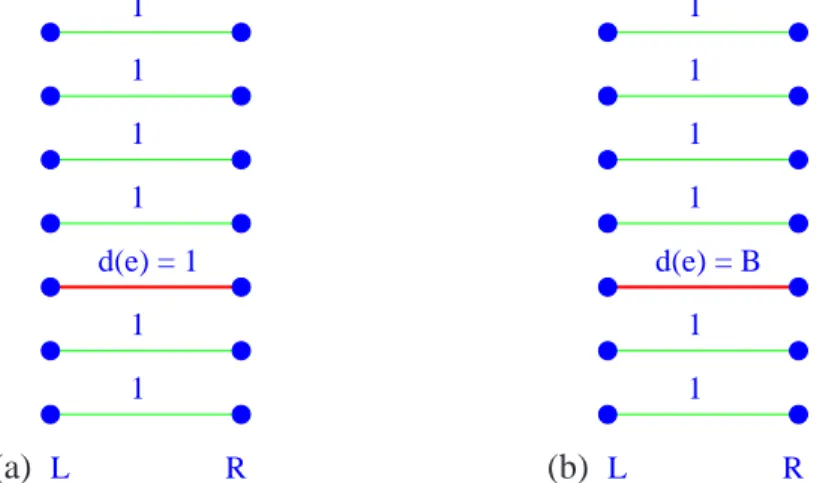
(a) L R 1
1 1 1
1 1 d(e) = 1
(b) L R
1 1 1 1
1 1 d(e) = B
Figure 3: Two instance of the metric matching which are indistinguishable in o(n2)time and whose cost
differ by a factor greater thanλ. The perfect matching connectingLwithRis selected at random and the edgeeis selected as a random edge from the matching. We setB =n(λ−1) + 2. The distances not shown are all equal ton3λ.
time a set of O(k) centers that are a constant factor approximation to the k-median objective
function. Later, standard constant factor approximation algorithms were given that run in time
e
O(n k) (see, e.g., [44, 50]). These sublinear-time results have been extended in many different
ways, e.g., to efficient data streaming algorithms and very fast algorithms for Euclideank-median
and also tok-means, see, e.g., [9, 12, 16, 27, 35, 36, 41, 42, 45]. For another clustering problem,
the min-sum k-clustering problem (which is complement to the Max-k-Cut), for the basic case
of k = 2, Indyk [39] (see also [38]) gave a (1 +ǫ)-approximation algorithm that runs in time
O(21/ǫO(1)
n(logn)O(1)), which is sublinear in the full input description size. No such results are
known for k ≥ 3, but recently, [22] gave a constant-factor approximation algorithm for min-sum
k-clustering that runs in timeO(n k(k logn)O(k))and a polylogarithmic approximation algorithm
running in timeOe(n kO(1)).
4.5
Limitations: What Cannot be done in Sublinear-Time
The algorithms discussed in the previous sections may suggest that many optimization problems in metric spaces have sublinear-time algorithms. However, it turns out that the problems listed in the previous sections are more like exceptions than a norm. Indeed, most of the problems have a trivial lower bound that exclude sublinear-time algorithms. We have already mentioned in Section
4 that the problem of approximating the cost of the lightest edge in a finite metric space (P, d)
requires Ω(n2), even if randomization is allowed. The other problems for which no
sublinear-time algorithms are possible include estimation of the cost of minimum-cost matching, the cost of minimum-cost bi-chromatic matching, the cost of minimum non-uniform facility location, the cost
ofk-median fork=n/2; all these problems requireΩ(n2)(randomized) time to estimate the cost
of their optimal solution to within any constant factor [10].
indistin-guishable by anyo(n2)-time algorithm for which the cost of the minimum-cost matching in one
instance is greater than λ times the one in the other instance (see Figure 3). Consider a metric
space (P, d)with 2n points, n points in L and n points in R. Take a random perfect matching
M between the points inL andR, and then choose an edgee ∈ Mat random. Next, define the
distance in(P, d)as follows:
• d(e)is either1orB, where we setB =n(λ−1) + 2,
• for anye∗M\ {e}setd(e∗) = 1, and
• for any other pair of pointsp, q ∈P not connected by an edge fromM,d(p, q) = n3λ.
It is easy to see that both instances define properly a metric space (P, d). For such problem
instances, the cost of the minimum-cost matching problem will depend on the choice of d(e): if
d(e) = B then the cost will ben−1 +B > n λ, and ifd(e) = 1, then the cost will ben. Hence,
any λ-factor approximation algorithm for the matching problem must distinguish between these
two problem instances. However, this requires to find if there is an edge of lengthB, and this is
known to require timeΩ(n2), even if a randomized algorithm is used.
5
Conclusions
It would be impossible to present a complete picture of the large body of research known in the area of sublinear-time algorithms in such a short paper. In this survey, our main goal was to give some flavor of the area and of the types of the results achieved and the techniques used. For more details, we refer to the original works listed in the references.
We did not discuss two important areas that are closely related to sublinear-time algorithms: property testing and data streaming algorithms. For interested readers, we recommend the surveys in [7, 26, 30, 31, 40, 49] and [47], respectively.
References
[1] N. Alon, S. Dar, M. Parnas, and D. Ron. Testing of clustering. SIAM Journal on Discrete
Mathematics, 16(3): 393–417, 2003.
[2] N. Alon, W. Fernandez de la Vega, R. Kannan, and M. Karpinski. Random sampling and approximation of MAX-CSPs. Journal of Computer and System Sciences, 67(2): 212–243, 2003.
[3] N. Alon, E. Fischer, M. Krivelevich, M. Szegedy. Efficient testing of large graphs.
Combina-torica, 20(4): 451–476, 2000.
[4] N. Alon, E. Fischer, I. Newman, and A. Shapira. A combinatorial characterization of the testable graph properties: it’s all about regularity. Proceedings of the 38th Annual ACM
[5] N. Alon and A. Shapira. Every monotone graph property is testable. Proceedings of the 37th
Annual ACM Symposium on Theory of Computing (STOC), pp. 128–137, 2005.
[6] N. Alon and A. Shapira. A characterization of the (natural) graph properties testable with one-sided error. Proceedings of the 46th IEEE Symposium on Foundations of Computer Science
(FOCS), pp. 429–438, 2005.
[7] N. Alon and A. Shapira. Homomorphisms in graph property testing - A survey. Electronic
Colloquium on Computational Complexity (ECCC), Report No. 85, 2005.
[8] S. Arora, D. R. Karger, and M. Karpinski. Polynomial time approximation schemes for dense
instances ofN P-hard problems. Journal of Computer and System Sciences, 58(1): 193–210,
1999.
[9] V. Arya, N. Garg, R. Khandekar, A. Meyerson, K. Munagala, and V. Pandit. Local search heuristics for k-median and facility location problems. Proceedings of the 33rd Annual ACM
Symposium on Theory of Computing (STOC), pp. 21–30, 2001.
[10] M. B˘adoiu, A. Czumaj, P. Indyk, and C. Sohler. Facility location in sublinear time.
Proceed-ings of the 32nd Annual International Colloquium on Automata, Languages and Programming (ICALP), pp. 866-877, 2005.
[11] C. Borgs, J. Chayes, L. Lov´asz, V. T. Sos, B. Szegedy, and K. Vesztergombi. Graph limits and parameter testing. Proceedings of the 38th Annual ACM Symposium on Theory of Computing
(STOC), 2006.
[12] M. Charikar, L. O’Callaghan, and R. Panigrahy. Better streaming algorithms for clustering problems. Proceedings of the 35th Annual ACM Symposium on Theory of Computing (STOC), pp. 30–39, 2003.
[13] B. Chazelle and D. P. Dobkin. Intersection of convex objects in two and three dimensions.
Journal of the ACM, 34(1): 1–27, 1987.
[14] B. Chazelle, D. Liu, and A. Magen. Sublinear geometric algorithms. SIAM Journal on
Computing, 35(3): 627–646, 2006.
[15] B. Chazelle, R. Rubinfeld, and L. Trevisan. Approximating the minimum spanning tree weight in sublinear time. SIAM Journal on Computing, 34(6): 1370–1379, 2005.
[16] K. Chen. Onk-median clustering in high dimensions. Proceedings of the 17th Annual
ACM-SIAM Symposium on Discrete Algorithms (SODA), pp. 1177–1185, 2006.
[17] A. Czumaj, F. Erg¨un, L. Fortnow, A. Magen, I. Newman, R. Rubinfeld, and C. Sohler. Sublinear-time approximation of Euclidean minimum spanning tree. SIAM Journal on
[18] A. Czumaj and C. Sohler. Property testing with geometric queries. Proceedings of the 9th
Annual European Symposium on Algorithms (ESA), pp. 266–277, 2001.
[19] A. Czumaj and C. Sohler. Estimating the weight of metric minimum spanning trees in sublinear-time. Proceedings of the 36th Annual ACM Symposium on Theory of Computing
(STOC), pp. 175–183, 2004.
[20] A. Czumaj and C. Sohler. Sublinear-time approximation for clustering via random sampling.
Proceedings of the 31st Annual International Colloquium on Automata, Languages and Pro-gramming (ICALP), pp. 396–407, 2004.
[21] A. Czumaj and C. Sohler. Abstract combinatorial programs and efficient property testers.
SIAM Journal on Computing, 34(3): 580–615, 2005.
[22] A. Czumaj and C. Sohler. Small space representations for metric min-sum k-clustering and
their applications. Manuscript, 2006.
[23] A. Czumaj, C. Sohler, and M. Ziegler. Property testing in computational geometry.
Proceed-ings of the 8th Annual European Symposium on Algorithms (ESA), pp. 155–166, 2000.
[24] M. Dyer, N. Megiddo, and E. Welzl. Linear programming. In Handbook of Discrete and
Computational Geometry, 2nd edition, edited by J. E. Goodman and J. O’Rourke, CRC Press,
2004, pp. 999–1014.
[25] U. Feige. On sums of independent random variables with unbounded variance and estimating the average degree in a graph. SIAM Journal on Computing, 35(4): 964–984, 2006.
[26] E. Fischer. The art of uninformed decisions: A primer to property testing. Bulletin of the
EATCS, 75: 97–126, October 2001.
[27] G. Frahling and C. Sohler. Coresets in dynamic geometric data streams. Proceedings of the
37th Annual ACM Symposium on Theory of Computing (STOC), pp. 209–217, 2005.
[28] A. Frieze and R. Kannan. Quick approximation to matrices and applications. Combinatorica, 19(2): 175–220, 1999.
[29] A. Frieze, R. Kannan, and S. Vempala. Fast Monte-Carlo algorithms for finding low-rank approximations. Journal of the ACM, 51(6): 1025–1041, 2004.
[30] O. Goldreich. Combinatorial property testing (a survey). In P. Pardalos, S. Rajasekaran, and J. Rolim, editors, Proceedings of the DIMACS Workshop on Randomization Methods in
Algo-rithm Design, volume 43 of DIMACS, Series in Discrete Mathetaics and Theoretical Computer Science, pp. 45–59, 1997. American Mathematical Society, Providence, RI, 1999.
[31] O. Goldreich. Property testing in massive graphs. In J. Abello, P. M. Pardalos, and
M. G. C. Resende, editors, Handbook of massive data sets, pp. 123–147. Kluwer Academic Publishers, 2002.
[32] O. Goldreich, S. Goldwasser, and D. Ron. Property testing and its connection to learning and approximation. Journal of the ACM, 45(4): 653–750, 1998.
[33] O. Goldreich and D. Ron. A sublinear bipartiteness tester for bounded degree graphs.
Com-binatorica, 19(3):335–373, 1999.
[34] O. Goldreich and D. Ron. Approximating average parameters of graphs. Electronic
Collo-quium on Computational Complexity (ECCC), Report No. 73, 2005.
[35] S. Har-Peled and S. Mazumdar. Coresets fork-means andk-medians and their applications.
Proceedings of the 36th Annual ACM Symposium on Theory of Computing (STOC), pp. 291–
300, 2004.
[36] S. Har-Peled and A. Kushal. Smaller coresets fork-median andk-means clustering.
Proceed-ings of the 21st Annual ACM Symposium on Computational Geometry, pp. 126–134, 2005.
[37] P. Indyk. Sublinear time algorithms for metric space problems. Proceedings of the 31st
Annual ACM Symposium on Theory of Computing (STOC), pp. 428–434, 1999.
[38] P. Indyk. A sublinear time approximation scheme for clustering in metric spaces. Proceedings
of the 40th IEEE Symposium on Foundations of Computer Science (FOCS), pp. 154–159, 1999.
[39] P. Indyk. High-Dimensional Computational Geometry. PhD thesis, Stanford University, 2000.
[40] R. Kumar and R. Rubinfeld. Sublinear time algorithms. SIGACT News, 34: 57–67, 2003.
[41] A. Kumar, Y. Sabharwal, and S. Sen. A simple linear time (1 + ε)-approximation
algo-rithm fork-means clustering in any dimensions. Proceedings of the 45th IEEE Symposium on
Foundations of Computer Science (FOCS), pp. 454–462, 2004.
[42] A. Kumar, Y. Sabharwal, and S. Sen. Linear time algorithms for clustering problems in any dimensions. Proceedings of the 32nd Annual International Colloquium on Automata,
Languages and Programming (ICALP), pp. 1374–1385, 2005.
[43] L. Lov´asz and B. Szegedy. Graph limits and testing hereditary graph properties. Technical Report, MSR-TR-2005-110, Microsoft Research, August 2005.
[44] R. Mettu and G. Plaxton. Optimal time bounds for approximate clustering. Machine
Learn-ing, 56(1-3):35–60, 2004.
[45] A. Meyerson, L. O’Callaghan, and S. Plotkin. A k-median algorithm with running time
independent of data size. Machine Learning, 56(1–3): 61–87, July 2004.
[46] N. Mishra, D. Oblinger, and L. Pitt. Sublinear time approximate clustering. Proceedings of
[47] S. Muthukrishnan. Data streams: Algorithms and applications. In Foundations and Trends in
Theoretical Computer Science, volume 1, issue 2, August 2005.
[48] M. Parnas, D. Ron, and R. Rubinfeld. Tolerant property testing and distance approximation.
Electronic Colloquium on Computational Complexity (ECCC), Report No. 10, 2004.
[49] D. Ron. Property testing. In P. M. Pardalos, S. Rajasekaran, J. Reif, and J. D. P. Rolim, editors, Handobook of Randomized Algorithms, volume II, pp. 597–649. Kluwer Academic Publishers, 2001.
[50] M. Thorup. Quickk-median,k-center, and facility location for sparse graphs. SIAM Journal
on Computing, 34(2):405–432, 2005.