Time-Consistent Institutional Design
∗
Charles Brendon
†Martin Ellison
‡January 20, 2015
This paper reconsiders normative policy design in environments subject to time incon-sistency problems, à la Kydland and Prescott (1977). In these environments there are generally gains to making binding promises about future policy conduct, in the form of an institutional target or mandate. However decisionmakers at different points in time have different preferences about the best promises to make and to keep. We consider the implications of choosing these promises according to a Pareto criterion. A sequence of promises is Pareto efficient if there is no alternative sequence that all current and fu-ture policymakers would prefer to switch to. This criterion has the advantage that it can be applied recursively, in environments where, by definition, no policy is recursively Ramsey-optimal. Recursive Pareto efficiency thus provides an appealing normative al-ternative to standard Ramsey policy. We characterise outcomes in a general setting when promises are chosen to be recursively Pareto efficient. Three examples, explored through-out the paper, highlight how this approach to policy design avoids features of Ramsey policy that are commonly identified as problematic.
Keywords: Institutional Design; Pareto Efficiency; Ramsey Policy; Time-Consistency JEL Codes: D02, E61
∗This is a very substantially revised version of a manuscript previously circulated under the title ‘Optimal Policy behind a Veil of Ignorance’. We thank Árpád Ábrahám, Paul Beaudry, Vasco Carvalho, Giancarlo Corsetti, Tatiana Damjanovic, Paul Levine, Albert Marcet, Ramon Marimon, Alex Mennuni, Meg Meyer, Michel Normandin, Ctirad Slavik, Rick Van der Ploeg and Simon Wren-Lewis for detailed discussions and comments, together with numerous seminar participants. All errors are ours.
†Faculty of Economics and Queens’ College, University of Cambridge. Email: [email protected]
1. Introduction
Time-inconsistency problems of the type first highlighted by Kydland and Prescott (1977) are a domi-nant feature of the modern macroeconomic policy literature. Whenever expectations of future policy influence the feasible set of current choices, period-by-period discretionary policymaking will gener-ically be sub-optimal. This is because successive generations of decisionmakers fail to endogenise the effects of their current choices on past expectations.
A general feature of these settings is that all generations can be made better off if some way can be found to commit to binding policy promises.1 A binding inflation target, for instance, can im-ply lower inflation expectations and a permanently improved inflation-output trade-off. A binding promise to limit future wealth taxation can ensure higher contemporary savings. To be effective these promises do not have to eliminate completely the scope for day-to-day policy choice, but they should restrict the options available. An inflation-targeting central bank retains operational independence, but is constrained by its obligation to target inflation.
The current paper takes as given that this sort of institutional commitment is possible, and revisits the policy question that it implies: How should such promises be designed? This is a non-trivial normative problem, because each generation of policymakers will have different preferences about the appropriate promises to make, and to keep, over time. Every generation would prefer that they themselves should be entirely free from promise-keeping obligations, but that their successors should be meaningfully restricted.
In this context it is impossible to find a sequence of promises that is recursively optimal: best for the first policymaker to choose, and best for all subsequent policymakers to adhere to. Choice must instead satisfy some weaker notion of desirability. The standard approach in the optimal policy literature is to relax recursivity, and to focus on the choice of promises that is optimal for the model’s first time period. This is commonly known as Ramsey policy.
This paper sets out an alternative approach. We define and characterise policy when promises are not chosen to be ‘best’ in any one time period, but must remain meaningfully desirable in all periods. In direct contrast with Ramsey policy, therefore, we retain recursivity in the choice procedure, but relax optimality. The criterion that we use in place of optimality is a version of the standard Pareto principle, taken with respect to the varying preferences of successive generations over promises. A choice is Pareto efficient if there is no other promise sequence that all current and future policymakers would prefer to switch to. It is recursively Pareto efficient if this statement remains true indefinitely, as the current period advances.
Our main motivation for developing this choice procedure is that a number of different literatures have found Ramsey policies to be unappealing. Two particular issues arise. First, in models of monetary and fiscal policy it is common for Ramsey promises to induce very different policies in early time periods from later, even though the underlying state of the economy may not have changed at all. Intuitively this is because Ramsey policy will never be constrained by inherited promises in the
1The formal insight that promises can be used to improve inefficient outcomes derives from the influential work of Abreu, Pearce and Stachetti (1990) on repeated games. There have been many applications in the macroeconomics literature, including Kocherlakota (1996), Chang (1998) and Phelan and Stachetti (2001).
first time period, but will subsequently. The associated transition dynamic makes it hard to infer simple rules of best conduct that could be used to design mandates for policymaking institutions. The Ramsey-optimal inflation target, for instance, is likely to vary from one time period to another even when the economy’s state vector does not. This problem has received particular attention in the New Keynesian literature, where Woodford (1999, 2003) has expressed the need for a ‘timeless’ approach to policy design, linking promises only to the state of the economy.
The second unappealing feature of Ramsey policy is that it can imply long-run outcomes that are extremely undesirable from the perspective of later generations. This is most commonly observed in the dynamic social insurance literature. In a dynamic hidden action model, Thomas and Worrall (1990) first showed that a Ramsey planner would promise to drive the consumption of almost all agents to zero over time. This ‘immiseration’ result was extended to general equilibrium in a hidden information setting by Atkeson and Lucas (1992), and has generated significant attention in the recent dynamic public finance literature.2 Again, it obtains even though the state of the economy may be precisely the same in the long run as at the start of time. Influential contributions by Phelan (2006) and Farhi and Werning (2007) have explored alternative normative criteria that would prevent the result from going through, in both cases based on an increase in the social discount factor.
The recursive Pareto approach that we present avoids these two unappealing features of Ramsey policy by design. First, because the Pareto criterion must continue to apply in every time period, for a given state of the economy there is no reason why policy should take a different form in early periods from later. Thus the policy transition can be avoided. Second, because the choice of promises must remain Pareto efficient indefinitely, outcomes that are extremely undesirable for later generations will not arise.
Our paper defines and characterises recursive Pareto efficiency as a way to choose promises, both in a general setting and by reference to three worked examples drawn from different branches of the optimal policy literature. These are, first, a linear-quadratic New Keynesian inflation bias problem; second, a variant of the Judd (1985) capital tax problem; and, third, a dynamic social insurance prob-lem under limited commitment, in the style of Kocherlakota (1996). To keep the arguments simple we focus on environments without aggregate risk.
An important feature of our work is the central focus that we place on promises as objects of anal-ysis. This follows from a novel decomposition of generic Kydland and Prescott problems that we provide. We split the policy choice procedure into two components. The first, an ‘inner problem’, considers the best way to select the day-to-day aspects of policy, given an exogenous sequence of promises that must be kept each time period. We show that this inner problem is fully time consis-tent. It concerns the aspects of choice that remain once expectations have been fixed. The second component, the ‘outer problem’, considers how the promises themselves should be chosen. This corresponds to the practical problem of designing an institutional mandate. Under conventional re-strictions the solution to the inner problem defines a well-behaved indirect utility function over the set of possible current and future promises. That is, it defines preferences over promises. These pref-erences will differ from one period to the next, as the benefits from issuing promises are superseded by the costs of keeping them. We analyse recursive Pareto efficiency in terms of these preferences.
The principal advantage of this decomposition is that it isolates the time-inconsistent aspects of choice for special treatment. It is only promises that will be chosen by a recursive Pareto criterion, since it is only the choice of promises that is time-inconsistent. Given the chosen promise sequence, all other variables will be recursively optimal. In environments that do not exhibit any time incon-sistency there will be no role for promises, and our method will, trivially, deliver standard optimal policies. As we discuss below, this is not true of alternative proposals in the literature.
Our main general characterisation result, presented in Section 5, relates to the properties of re-cursively Pareto efficient promises in steady state. We show this steady state, if it exists, will differ systematically from the steady state of Ramsey policy. Specifically, less weight will be put on the value of manipulating past expectations. This is true in a precise sense. Whereas under Ramsey pol-icy the shadow value associated with past promises will generally be a non-stationary object,3under recursively Pareto efficient policy it decays over time at rateβ– the discount factor.
Under slightly more restrictive assumptions we additionally prove a sufficiency result: any promises inducing convergence to a steady state of the form that we characterise must be recursively Pareto efficient. One implication of this is that recursive Pareto efficiency will usually be satisfied by mul-tiple promise sequences, but we propose simple ways to resolve this multiplicity, motivated by our desire to find policies that vary in the state of the economy only. In models without any state vari-ables we show that the policy that is best in the set of time-invariant choices is also recursively Pareto efficient, and this is not true of any other constant policy. We focus attention on this choice. In models with endogenous state variables we argue that there remain good reasons for considering constant promises, even though day-to-day choices must vary with the state of the economy.
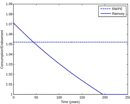
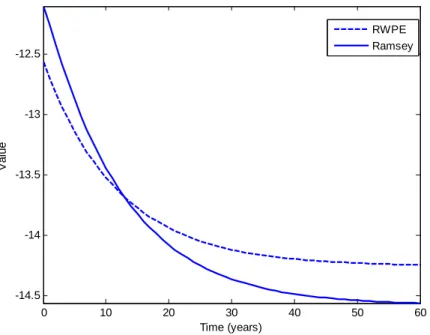
Turning to the specific examples, we show that recursively Pareto efficient policy justifies a con-stant, slightly positive inflation target in the basic linear-quadratic New Keynesian problem.4 This contrasts with a Ramsey promise path in which inflation starts at a higher rate but gradually decays to zero. The loss associated with recursively Pareto efficient policy is initially above the loss from Ramsey, but after a finite length of time it becomes less appealing to continue with the Ramsey plan. In the capital tax example we show that recursively Pareto efficient promises deliver convergence to a steady state with mild positive capital taxes – around 28 per cent of net capital income in the calibration we use. Tax rates vary with the capital stock, but within relatively small bounds. A deviation of the capital stock of five per cent from steady state causes capital tax rates to differ by about two percentage points. This contrasts with Ramsey policy, which requires initial capital tax rates of around 300 per cent of the tax base, gradually decaying to zero.5 This result obtains even if the initial capital stock starts in its long-run steady-state level.6
3This is known from the work of Marcet and Marimon (2014).
4Recall that the basic linear New Keynesian Phillips Curve takes the form:
πt =βEtπt+1+γyt
where inflation isπt, the output gap isyt andβandγare parameters. Since genericallyβ ∈ (0, 1), this exhibits a
long-run trade-off between inflation and output. Thus permanently positive inflation is associated with a permanently positive output gap.
5The tax base is net capital income, so tax rates in excess of 100 per cent imply that underlying capital assets are being taxed.
The finding that steady-state taxes are positive under recursively Pareto efficient policy is an im-portant one because it emphasises that the celebrated ‘zero capital tax’ steady-state outcome under Ramsey policy, first identified by Judd (1985), cannot be viewed as desirable in isolation from the high-tax transition to it. Part of the reason why long-run capital taxes are held so low under Ramsey policy is to ensure that high initial capital levies will not discourage savings to too great an extent. When policy is recursively Pareto efficient, high initial rates do not form part of the chosen plan. This reduces the need for early generations to be given incentives to save. Long-run capital taxes are higher as a consequence.
The model of social insurance with participation constraints provides a simple setting in which long-run outcomes are clearly undesirable under Ramsey policy. We assume that a fixed fraction of the population is permanently income-poor, and a utilitarian government would like to provide some degree of redistribution to these agents. Initially a Ramsey planner does this by redirecting to them some of the surplus raised by providing consumption insurance to the rest of the population, whose incomes are stochastic. Over time, however, the resources available for redistribution disappear. This is because initial high earners are promised high long-run utility levels, as compensation for the large payments they make to the scheme. Making good on these promises means it eventually becomes too costly to provide any further redistribution to low earners.
When promises are instead chosen to be recursively Pareto efficient, redistribution to low earners is a feature of policy at every horizon. The chosen allocation is the best feasible stationary consumption distribution. Again, after a sufficient amount of time has passed it becomes preferable for all current and future policymakers to switch away from the continuation of Ramsey policy, to the policy that is recursively Pareto efficient.
1.1. Relation to literature
Many economists have expressed unease about the Ramsey approach to choice under time inconsis-tency. Svensson (1999) puts the problem succinctly, asking ‘Why is period zero special?’ The idea that preferences in some initial time period should be privileged above others does not seem con-sistent with the way that policy is, or should be, designed in practice. A large body of work has responded by supposing that choice must be made on a period-by-period basis, and analysing the resulting outcomes. An early branch of this literature, led by Chari and Kehoe (1990) and Atkeson (1991), investigated the set of reputational equilibria that could be supported in these settings by ap-propriate trigger strategies, which allowed for limited improvements on Markov-perfect equilibria.7 More recently, a large number of papers have computed the properties of Markov-perfect equilibria, highlighting the inefficiencies that result.8
the Judd (1985) model, with the economy instead collapsing to a corner solution under conventional parameterisations. Our version of the model differs from theirs in two regards. First, it is a representative-agent economy: there is no capitalist-worker distinction. Second, labour supply is endogenous. Together these features imply a zero steady-state capital tax rate for the standard calibrations we use.
7Important papers by Sleet and Yeltekin (2006) and Golosov and Iovino (2014) have placed particular attention on the best equilibria that are supportable in this way.
8Examples include Klein and Ríos-Rull (2003), Ortigueira (2006), Ellison and Rankin (2007), Klein, Krusell and Ríos-Rull (2008), Díaz-Giménez et al. (2008), Martin (2009), Blake and Kirsanova (2012), Reis (2013) and Niemann et al. (2013).
Our work shares with this literature an unease about the special treatment Ramsey policy gives to the first policymaker. Where it differs is in continuing to ask a normative question: Howshould policy be designed, given that we do not want period zero to be treated as special? This is different from asking what sorts of policies could be expected to follow if there were no formal commitment device.
When commitment devices are assumed, different branches of the literature have addressed per-ceived problems with Ramsey policy on a largely case-by-case basis, depending on whether it is the long-run outcome or transition dynamics that appear more implausible. Influential work by Phe-lan (2006) and Farhi and Werning (2007) has placed particular focus on strategies for avoiding the immiseration result in the model of Atkeson and Lucas (1992). These authors proceed by attaching distinct non-zero Pareto weights to later generations when designing social insurance policy. Phelan considers policy that maximises steady-state welfare, whereas Farhi and Werning focus on a broader Pareto set. Both approaches are equivalent to increasing the social discount factor above its private-sector value, so that the government values later generations more than private individuals do. As an approach this is indeed sufficient to overturn immiseration, but its implications stretch far wider. It implies a change to dynamic decisionmaking even in models where no Kydland and Prescott prob-lem is present. In a textbook Ramsey growth model, for instance, it would mandate a higher savings rate for any given capital stock.
An important message of our paper is that the question of how best to resolve time inconsistency can be separated from the broader question of how best to discount the future. The main differ-ence between our work and that of Phelan (2006) and Farhi and Werning (2007) is that we depart from standard choice procedures only in our treatment of promises. For this, the decomposition of choice into a time-consistent ‘day-to-day’ choice problem, and a time-inconsistent ‘institutional de-sign’ problem is essential. It allows us to focus our attention exclusively on the time-inconsistent aspects of choice. Capital accumulation decisions, for instance, will not be affected directly by what we do. There are also important differences between the Pareto criterion that we apply and the cri-terion that Farhi and Werning (2007) use, based on the treatment of endogenous state variables. This is a necessarily technical matter, and we defer a full discussion of it to Section 4.
The other body of work that has considered normative alternatives to Ramsey policy is the New Keynesian monetary policy literature. Here, by contrast, it is the fact that Ramsey policy comes with transition dynamics that is identified as problematic. To address this, Woodford (1999, 2003) has advocated a ‘timeless’ approach to policy design, which involves implementing steady-state Ramsey policy from the start of time.9The capital tax literature often proceeds in similar fashion, albeit more informally, with high taxes along the transition generally being neglected for the purposes of policy advice.10 But the justification for these approaches is unclear. There is no particular reason why the
steady state of Ramsey policy should itself be desirable, independently of the transition. What if the long-run outcome of Ramsey policy is immiseration for almost all agents? Our paper differs from
9More recent papers in the New Keynesian tradition that follow this approach include Adam and Woodford (2012), Benigno and Woodford (2012), and Corsetti, Dedola and Leduc (2010). Damjanovic, Damjanovic and Nolan (2008) offer an alternative approach based on maximising steady-state welfare, influenced by results due to Blake (2001) that showed timeless perspective policy may not maximise expected welfare.
this literature in the way it derives transition-free policy directly from the application of a recursive normative criterion, rather than by augmenting Ramsey policyex-post.
1.2. Outline
The remainder of the paper proceeds as follows. Section 2 sets out the general problem that we study, and shows how this framework nests our three main examples. Section 3 explains the decom-position of the general problem into ‘inner’ and ‘outer’ components, and derives some important properties of the value function for the inner problem. Section 4 provides alternative definitions of Pareto efficiency that could be applied the outer problem, and explains why we favour what we label an ‘ex-post’ Pareto criterion. Section 5 characterises recursively Pareto efficient policy in steady state, highlighting its generic difference with Ramsey policy. Section 6 explores desirable selection proce-dures for obtaining a unique policy, and illustrates this policy in our three main examples. Section 7 concludes. All proofs are collected in an appendix.
2. General setup
Time is discrete, and runs from period 0 to infinity.11In each periodtthere exists a policymaker with
preferences over allocations from period t onwards. These allocations are of the form{xs+1,as}∞s=t
where xs ∈ X ⊂ Rn is a vector ofnstates determined in period s−1 and as ∈ A ⊂ Rm×Rς is a
vector of controls determined in periods. There aremcontrols, and each is defined for all possible realisations of a stochastic vectorσs∈Σ, whereΣis a countable set of cardinalityς. ςmay be infinite.
as(σs)∈Rmdenotes the value ofasparticular to the realisationσsof the stochastic process.
The policymaker’s preferences in periodtare described by a time-separable objective criterionWt:
Wt :=
∞
∑
s=t
βs−tr(xs,as). (1)
The policymaker is constrained by a set ofnrestrictions defining the evolution of the state vector:
xs+1=l(xs,as), (2)
a set oficontemporaneous restrictions linking controls and states:
p(xs,as)≥0, (3)
and ‘forward-looking’ constraints of two different types. The first is a set ofjtime-separable restric-tions looking forward over the infinite horizon:
Es
∞
∑
τ=1
βτh(as+τ(σs+τ),σs+τ) +h0(as(σs),σs)≥0, (4)
whereas the second is a set ofkrestrictions looking forward one period ahead:
Esβg1(as+1(σs+1),σs+1) +g0(as(σs),σs)≥0. (5)
It is assumed thatj+k≥1 so the policymaker is subject to at least one forward-looking constraint, but otherwise there is no requirement that any ofi,j,kormshould be non-zero. Constraints (2) to (5) hold for alls ≥tin periodt, with the functions in the constraints vector-valued and of the specified dimension. The values of the functions in (4) and (5) are allowed to vary directly in the vector of the exogenous stochastic processσs, as well as indirectly throughas(σs). Where the meaning is clear, we
will usually keep the dependence ofasonσsimplicit, writingh(as,σs)and so on.
The expectations in (4) and (5) are taken with respect to an ergodic Markov process forσsdefined
onΣ. The process has a time-invariant probability of transiting from stateσto stateσ0that is denoted
by P(σ0|σ)and a stationary probability of state σ denoted by P(σ). Constraints (4) and (5) must
hold for all initialσs ∈ Σ. By assumption there is no aggregate uncertainty. This approach to
mod-elling uncertainty is somewhat restrictive, but is economical on notation and sufficient to incorporate a number of important models. This includes the social insurance example below, where there is idiosyncratic income risk. It will be useful at times to make reference toA(σ)⊂ Rm as the space of
control variables available for a givenσdraw.
The distinction between restrictions that are infinite-horizon and one-period ahead in (4) and (5) is made because these are the two main forms of forward-looking constraints in most problems of interest. This is without loss of generality. Intermediate cases in which outcomes insare constrained by expectations of outcomes up to finite horizons+ncan be written in the form of (5), by defining appropriate auxiliary variables and additional contemporaneous restrictions of the form in (2) link-ing these auxiliary variables to the controls. Similarly, the absence of state variables from forward-looking constraints is without loss of generality when appropriate auxiliary variables and additional contemporaneous restrictions are likewise defined.
It is constraints of the form (4) and (5) that are responsible for time inconsistency. The policymaker in periodtis not restricted to ensure that the versions of these constraints relating tot−1 and earlier remain satisfied, and in general it will be best to renege on any past promises to do so. This was the problem highlighted by Kydland and Prescott (1977). The next section briefly introduces three examples that can be nested in the general setup.
2.1. Three examples
Example 1: A linear-quadratic ination bias problem
Allocations in periodtconsist of inflationπt and the output gapyt. These are both control variables
so there are no state variables. The policymaker’s objective is: −
∞
∑
s=t βs−t
h
πs2+χ(ys−y¯)2
i
whereχ >0 is a parameter and ¯y > 0 is the optimal level for the output gap.12 The policymaker is
subject to a single constraint, a deterministic version of the New Keynesian Phillips curve. This is a one-period ahead restriction of the form in (5):
πs =βπs+1+γys, (7)
withγa parameter. This forward-looking constraint provides an incentive to promise low inflation
in the future so as to ease the current inflation-output trade-off. Such a promise is generally time-inconsistent. Full details can be found in Woodford (2003).
Example 2: A capital tax problem
This is a variant of the balanced-budget problem studied by Judd (1985). A representative agent consumes, saves and supplies labour. For exogenous reasons, the government must consume a fixed quantity g of real resources each period. Government consumption is funded by a linear tax on labour income and a linear tax on capital income net of depreciation. The government cannot borrow. Allocations in periodt are consumptionct, labour lt, output yt and the capital stockkt. The capital
stock is the only state variable and the rest are controls. The policymaker’s objective in periodtis to maximise the lifetime utility of the representative agent:
∞
∑
s=t
βs−tu(cs,ls) (8)
The policymaker faces an aggregate resource constraint of the form in (2):
ks+1=ys−cs−g+ (1−δ)ks, (9)
and a production constraint of the form in (3):
ys ≤F(ks,ls). (10)
The distortionary character of taxes implies a further ‘implementability’ constraint that restricts allo-cations available to the policymaker when the problem is written as here in its primal form.13 In the present case this is a one-period ahead forward-looking restriction of the form in (5):14
β{uc,s+1(cs+1+ks+2) +ul,s+1ls+1} ≥uc,sks+1 (11)
This constraint says that the value of consumption and capital purchases in periods+1, net of any
12This exceeds the natural level of output due to monopoly power in the product market. 13See Chari and Kehoe (1999).
14Strictly this differs in form from (5) in containing state variables, and a variable dated at s+2. Using the resource constraint (9) we can rewrite the condition as:
βuc,s+1(ys+1−g+ (1−δ)zs+1) +ul,s+1ls+1 ≥uc,s[ys−cs−g+ (1−δ)zs],
labour income that period, must weakly exceed the value of the capital holdings that are taken into period s+1, where these values are calculated in period s at prices corresponding to anticipated marginal rates of substitution. In short, it prevents the policymaker from restricting the consumer’s spending powerex postrelative to what is anticipated. This will conflict with the incentive of a later policymaker to tax the consumer’s existing, inelastic capital holdings.
Example 3: Social insurance with participation constraints
This is a variant of the limited commitment model due to Kocherlakota (1996). There is a contin-uum of agents indexed on the unit interval, with each agent receiving an endowment each period. Measureµ∈[0, 1)of agents receive a low incomeyl in every period. The remaining measure(1−µ)
receive a high incomeyh >ylwith probabilitypin a given period, and a low incomeylwith
probabil-ity(1−p). The endowment draws are independent across agents and time, and publicly observable. The Ramsey-optimal plan in this environment has the consumption levels of agents subject to in-come risk depending only on the time elapsed since those agents last received a high-inin-come draw, so attention is restricted to policies with this feature.15 The exogenous stochastic variableσs,i ∈ Σ
can then be defined as the number of periods since agentilast drew a high income, withΣthe set of positive integers (including 0). The Markov process governingσs,ifor generic agentiis:
σs,i+1=
σs,i+1 with prob (1−p)
0 with prob p
.
Agents subject to income risk are only differentiated by the time since they last had a high-income draw, and hence can be indexed by theirσs,ivalues.16 Furthermore, the stochastic process governing σs,i implies that there will be measure(1−µ) (1−p)σpof agents in each period who last received a
high-income drawσperiods ago.
The policymaker’s objective in periodtis utilitarian: ∞
∑
s=t βs−t
"
(1−µ)
∞
∑
σ=0
(1−p)σ
pu(cs(σ)) +µu(cps)
#
, (12)
where cs(σ)is the consumption in period s of an agent who received a high-income draw σ
peri-ods ago, andcspis the consumption in periodsof an agent who has a permanently low income. The
utility functionusatisfies the usual properties. The problem has interesting properties without incor-porating public or private asset accumulation, so the resource constraint is assumed to hold period
15This is done mainly to keep the notation simple, since for these policies it is sufficient for the policymaker to summarise an agent’s history up to periodsin the single variableσs,i. The results obtained do not change when more general forms
of dependence are formally allowed.
16For simplicity, it is assumed that information on the infinite history of endowment draws is available from the start of time. This information will be irrelevant to the Ramsey plan, but may be of use in designing a stationary policy. It would make no difference to the argument if this ‘information’ were fictitiously drawn according to the true underlying distribution in period 0.
by period:
(1−µ)
∞
∑
σ=0
(1−p)σ
pcs(σ) +µcsp ≤[1−(1−µ)p]yl+ (1−µ)pyh. (13)
Incentive compatibility requires the insurance scheme to deliver at least as much utility to an agent as they could obtain in autarky, which implies infinite-horizon forward-looking constraints of the form in (4):
Et
∞
∑
s=t
βs−tu(cs(σs,i))≥u(yt) + β
1−β
h
pu(yh) + (1−p)u(yl)i, (14) for agents drawing incomeyt, and
∞
∑
s=t
βs−tu(ctp)≥ 1
1−βu(y
l) (15)
for the permanently low income agents. These incentive compatibility constraints are the source of time inconsistency. The government has anex-anteincentive to minimise costs and maintain the social insurance scheme by promising high future utility to agents with a high income draw, but there will beex-postincentives to renege on these promises.
2.2. Assumptions
It is useful to describe a range of possible restrictions that can be placed on general functionsr,l,p, h,h0,g1andg0later in the analysis.
Assumption 1. The functions r : X×A → R, l : X×A → Rn, p : X×A → Ri, h : A(
σ) → Rj,
h0: A(σ)→Rj, g1 : A(σ)→Rk and g0 : A(σ)→Rkare continuous. The spaces A ⊂Rmand X ⊂Rn
are compact and convex.
Assumption 2. The functions r, l, p, h, h0, g1and g0are continuously differentiable.
Assumption 3. The functions h, h0, g1and g0are quasi-concave.
Assumption 4. The function r is strictly concave, the function p is quasi-concave and the function l is linear.
Assumption 5. The functions p, h, h0, g1and g0are concave.
Assumption 1 brings some basic structure to the problem and will be assumed throughout. In most environments of interest the relevant constraint functions are utility functions, production functions, profit functions and the like, for which continuity is a relatively innocuous imposition. Convexity and compactness are similarly conventional structures to impose on the spacesAandX. Assumption 2 is invoked principally for ease of exposition. It would be possible to relax it, but only at notational cost and without changing the character of the results, so it is likewise imposed throughout. Assump-tions 3, 4 and 5 are progressively stronger. In the capital tax example, for instance, it is unclear that the relevant functions in the implementability constraint (11) satisfy quasi-concavity, let alone full concavity. For an example of this type it will generally only be possible to confirm Assumptions 3 to 5 under specific functional forms.
5 10 15 20 25 30 0.5
1 1.5
Inflation
Time (years)
π
(
%
)
5 10 15 20 25 30
2 4 6 8
Output
Time (years)
y
(
%
d
e
v
.)
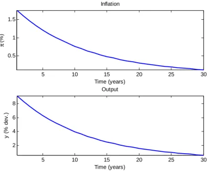
Figure 1: Ramsey paths for inflation and output in the linear-quadratic inflation bias problem The main purpose of Assumptions 3, 4 and 5 is to allow some structure to be placed on a class of indirect objective functions to be defined below. These will be central to the analysis of alternative normative strategies, and differing assumptions on the primitives will affect what can be said about efficient resolutions to the time inconsistency problem.
2.3. Ramsey policy
Ramsey policy is an allocation
xR s+1,aRs
∞
s=0that maximisesW0 subject to all relevant constraints of
the form (2) to (5) for alls ≥0. In general, the continuation of this policy
xsR+1,aRs ∞s=tfrom period t > 0 will not maximiseWtsubject to the same constraints being satisfied for s ≥ t. This is because
the Ramsey policy will have been influenced by a desire to affect expectational constraints that were binding in periods prior to t, but which are no longer a concern – the time inconsistency problem. The characteristics of Ramsey policy in the three examples are next introduced and discussed.
Example 1: A linear-quadratic ination bias problem
The Ramsey plan for the linear-quadratic inflation bias example is familiar from the New Keynesian literature.17 Figure 1 shows the dynamic paths of inflation and output under a conventional calibra-tion of β = 0.96,γ = 0.024, χ = 0.048, ¯y = 0.1. Initial choices are unconstrained by the effects of
current inflation on past expectations, meaning that the costs of engineering high output are initially quite low. The output gap is initially set above 9 per cent, after which it is optimal to allow inflation to drift downwards over time as lower future inflation permits higher current output under the New Keynesian Phillips Curve (7). In steady state the inflation rate is zero, as is the output gap.
0 10 20 30 40 50 60 100
200 300
Capital Taxes
Time (years)
τ
k (
%
)
0 10 20 30 40 50 60
0.95 0.96 0.97 0.98 0.99
Capital
Time (years)
k
(
%
o
f
s
s
v
a
lu
e
)
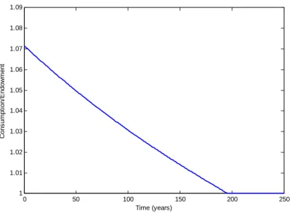
Figure 2: Ramsey capital taxes and the capital stock in the capital tax problem
Example 2: A capital tax problem
The Ramsey path in the capital tax example is plotted in Figure 2, assuming standard parameter values and functional forms.18 The initial capital stock is set equal to the Ramsey steady-state value, and plotted in the lower panel as a percentage of the steady-state capital stock. The broad properties of the Ramsey path are familiar from the literature following Chamley (1986) and Judd (1985). Initial taxes on net capital income are implausibly high, at around 300 per cent, but decay to zero as time progresses.19 The capital stock reflects the path of capital taxes, falling over the first 10 years to a
level about 5 per cent below its steady-state value as higher taxes reduce the incentives to save. The capital stock only gradually recovers afterwards as taxes fall and the incentives to save are restored.
Example 3: Social insurance with participation constraints
The general properties of social insurance models with participation constraints have been explored in a number of recent papers.20Figure 3 charts the dynamic consumption path of individuals whose income endowment is constrained to be low each period.21 These agents initially receive a significant transfer, raising their consumption to just below the average endowment in the economy.22 As time 18Specifically, utility takes an additively separable isoelastic form. Consumption utility is logarithmic and labour disutility is exponential, with an inverse Frisch elasticity equal to 2. The production function is Cobb-Douglas with capital share 0.33.β=0.96,δ=0.05 andg=0.6, which ensures a steady-state government consumption to output ratio of 0.31.
19There is no economic reason to rule out capital taxes in excess of 100 per cent, as agents can always meet the associated liabilities by selling their underlying capital holdings.
20Among others, see Krueger and Perri (2006), Krueger and Uhlig (2006), Broer (2013) and Ábrahám and Laczó (2014). 21The calibration uses log consumption utility with
β=0.96,µ=0.2,p=0.01,yl=1 andyh=10. Qualitative outcomes
are not strongly dependent on these choices.
22The average endowment is 1.072. A first-best utilitarian policy would provide this level of consumption to all agents in all periods.
0 50 100 150 200 250 1
1.01 1.02 1.03 1.04 1.05 1.06 1.07 1.08 1.09
Time (years)
C
o
n
s
u
m
p
ti
o
n
/E
n
d
o
w
m
e
n
t
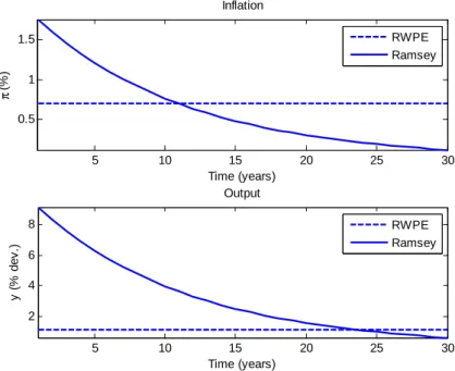
Figure 3: Consumption path for low-income agents in the social insurance problem
progresses, their consumption drifts down as transfers are instead directed towards satisfying the participation constraints of agents who have just received a high-income draw. The permanently low income agents are eventually limited to consuming only their endowment. An identical consumption trajectory is followed by an agent who is subject to income risk but is unlucky enough always to draw a low income.
Discussion: Asymmetric objectives and outcomes
An important characteristic of Ramsey policy in all three examples is its dynamic asymmetry. Ramsey-optimal inflation trends downwards in the linear-quadratic inflation bias example, even though the structure of this simple New Keynesian economy is entirely stationary. The same is true of optimal consumption for permanently low income agents in the social insurance example. The capital tax example features capital as an endogenous state variable, which could potentially account for some of the dynamics in policy choices. However, the calibration assumes that the initial capital stock is equal to its eventual steady-state value. Nonetheless, the character of the initial policy with capital taxes at 300 per cent could hardly be more different from that which obtains in the limit when capital taxes converge on zero. Thus in all three examples the Ramsey policy induces a different allocation in identical economic circumstances, dependent entirely on the amount of time that has progressed since optimisation took place.
The dynamic asymmetry of outcomes is unsurprising given the definition of Ramsey policy. No policy exists that is optimal in the set of possibilities from every time period onwards. The Ramsey approach selects a policy that is best from period 0 onwards, but this policy cannot also be best from generic periodsonwards, otherwise there would be no time-inconsistency problem. This implies that if the natural state of the economy is identical in periods 0 and sthen policies must differ between the two periods. Such asymmetry is an uncomfortable property for policy models to exhibit. It is
difficult, for instance, to imagine that a central bank might pursue a time-varying inflation target, or that capital taxes would follow the sort of trajectory exhibited in Figure 2.
What is needed is an approach to designing policy that delivers time-symmetric allocations whilst remaining meaningfully desirable. The question is what the relevant desirability concept ought to be. The ‘timeless perspective’ approach of Woodford (1999, 2003) proposes one answer that has been widely applied in the New Keynesian policy literature.23 It requires the policymaker in period 0 to immediately implement the steady-state allocations associated with Ramsey policy. Thus, Woodford (2003) would advocate an optimal inflation rate of zero in period 0 of the linear-quadratic inflation bias example. His heuristic justification is that the Ramsey steady-state policy is time-invariant, and would have formed part of a Ramsey-optimal path had optimisation taken place in the distant past. The resulting choices would have been optimal fromsometime perspective, albeit one prior even to the first period of the model. The same focus on Ramsey steady-state outcomes has been emphasised more informally in the dynamic capital tax literature, where policy recommendations have typically stressed the zero steady-state capital tax rates whilst discarding the associated transition to steady state.24
However, ‘Do what would have been planned for today in the distant past’ may not always be a desirable, or even feasible, maxim to follow. The example of social insurance with participation constraints sounds a particularly cautionary note. The permanently low income agents receive no transfers from their more fortunate peers in Ramsey steady state, and so are left consuming their low income endowment forever. Immediate implementation of the steady-state allocations would hence eliminate all the gains from redistribution that accrue during the first 200 ‘early’ years of the Ramsey policy. This is clearly not a desirable outcome. It is similarly unclear whether the Ramsey steady-state allocation can necessarily be implemented in period 0 when the policy environment in-cludes endogenous state variables. In a version of the social insurance problem with public storage and a sufficiently high real interest rate, the Ramsey-optimal policy involves the policymaker accu-mulating sufficient assets so that first-best complete risk-sharing is achieved in the long run.25 This clearly cannot be implemented from the very first time period if the policymaker has not yet accu-mulated sufficient assets. In examples such as these the timeless perspective policy does not seem well defined.26
The approach we take is to define a policy criterion that is weaker than ‘optimality’ but can still be applied recursively. We argue that a version of the Pareto criterion can do just this, providing a new systematic approach to institutional and policy design that delivers desirable time-symmetric allocations. To make progress, the next section distills the time inconsistency problem by separating
23Recent examples include Adam and Woodford (2012) and Corsetti, Dedola and Leduc (2010). Woodford (2010) provides a more detailed discussion of the merits of eliminating asymmetries over time.
24See Atkeson et al. (1999). Straub and Werning (2014) have recently highlighted the inseparability of transition dynamics from the optimality of the subsequent zero rate.
25Ljungqvist and Sargent (2012), Chapter 20, gives a textbook presentation of this result.
26From a technical perspective, it is known from the work of Marcet and Marimon (2014) that the Pareto weights of agents are non-stationary in the social insurance example with participation constraints. Woodford (2003) presents his approach as imposing steady-state values for the multipliers on past promises when solving the period 0 decision problem. But these multipliers are one and the same as the Pareto weights, and thus cannot take steady-state values because of their non-stationarity.
out the underlying choice variables to which time inconsistency is attached.
3. Inner and outer problems
The general problem can be divided into two components, an ‘inner’ and ‘outer’ problem.27 The outer problem is concerned with the selection of a dynamic path for promise variables. These corre-spond to the promise values used by Abreu, Pearce and Stachetti (1990) to give a recursive structure to the Ramsey problem, though they are not used here directly to obtain recursivity. Instead, the outer problem is one of choosing an entire time-contingent sequence of such promises, which we label an institutional design problem. An ‘inner’ problem can then be cast, determining the optimal dynamic allocation subject to the promise constraints given by the outer problem. The value of this inner problem is contingent on the given sequence of promises, and can be interpreted as an indirect utility function across possible promise sequences. The time inconsistency problem then manifests it-self as time variation in this preference structure, and conventional normative criteria, such as Pareto efficiency, can be used to assess the desirability of alternative institutions.
3.1. The inner problem
The inner problem solves for optimal allocations, conditional on feasibility and given sequences for the promise values. Mathematically, in periodt≥0 the inner problem solves:
max
{xs+1,as}∞s=t Wt :=
∞
∑
s=t
βs−tr(xs,as),
subject to the evolution of the state vector (2), the restrictions linking controls and states (3), and the promise constraints:
h0(as,σs) +βEωsh+1(σs+1) ≥ 0, (16)
h(as,σs) +βEωsh+1(σs+1) ≥ ωhs(σs), (17)
g0(as,σs) +βEωsg+1(σs+1) ≥ 0, (18)
g1(as,σs) ≥ ωgs(σs), (19)
for alls ≥t, wherext ∈ Xis the initial state vector andωsh(σs)∈Rjandωgs(σs)∈Rkare sequences
ofσ-contingent vectors for the promise values in alls≥ t.
The promise valuesωhs andωsgare stacked in the vector[ωsh(σs)0,ωsg(σs)0]0 := ωs(σs)∈Rj+kand
the collection of promise values acrossσs draws is denoted byωs := {ωs(σs)}σs∈Σ. Conditions (16) and (18) are ‘promise-making’ constraints, as they restrict the choice of variables in the h0 and g0
functions relative to a vector of future promise values. The implication is that future values of theh andg1functions must be at least as large as these promise values, in order for the full expectational
constraints to be satisfied. This is ensured by the ‘promise-keeping’ constraints (17) and (19).
For the original constraints (4) and (5) to hold for alls ≥ t, it is sufficient to ensure that (16) and (18) hold for all s ≥ t and (17) and (19) for all s > t. Imposing constraints (17) and (19) also for periodt would add an additional restriction on choice. This can be motivated by a need to respect past promises, but not by the fundamental economic restrictions that feature from periodtonwards.
3.1.1. Notation
The set of infinite promise sequences{ωs}∞s=tsuch that the inner problem has a non-empty constraint
set is denoted byΩ(xt)⊂ (Rj+k×Rς)∞, for an initial state vectorxt. The interior ofΩ(xt)is
repre-sented by ˚Ω(xt). Compactness ofAandXand the continuity properties imposed under Assumption
1 together imply that the constraint functions in (16) to (19) are bounded uniformly ins. This in turn means that sufficiently large, uniform bounds can be imposed on the values ofωhs(σs)andωsg(σs)
without affecting the problem. These bounds are incorporated into the definition ofΩ(xt):28
Assumption. {ωs}∞s=t∈Ω(xt)only if the sequence{ωs}∞s=tis uniformly bounded in s for all xt ∈X.
The value of the inner problem is denoted byV({ωs}∞s=t,xt), for allxt∈ Xand all{ωs}∞s=t ∈Ω(xt).
This object will be a major focus of the analysis, and we label it the ‘promise-value function’. Where convenient, the convention will be thatV({ωs}∞s=t,xt) = −∞when the inner problem has an empty
constraint set, which allowsVto be defined on the entire product space Rj+k×Rς∞
.
It will also be useful to consider the evolution of the state variables associated with any given promise sequence. We say that the sequence{ωs}∞s=tand initial statext‘induces’ a sequence of state
vectors{x0s+1}s∞=tif there exists a sequence of control variables{a0s}s∞=tsuch that{x0s+1,a0s}∞s=tsolves the inner problem for given{ωs}∞s=tandxt.
3.1.2. Time consistency
Proposition 1. The inner problem istime consistent. That is, if{x0s+1,a0s}∞s=t solves the inner problem for promise sequence {ωs}∞s=tand initial state vector xt, then the continuation{xs0+1,a0s}∞s=t+τ solves the inner
problem for promise sequence{ωs}∞s=t+τ and initial state vector x
0
t+τ for allτ≥1.
The proof is straightforward and given in the appendix. Time consistency is an important prop-erty of the inner problem. The essential point is that time inconsistency problems derive from dif-ferent policymakers having difdif-ferent incentives to make, keep and renege uponpromises. Once these promises are treated as given, no additional source of time inconsistency remains.
3.2. Properties of the promise-value function
The promise-value functionV({ωs}∞s=t,xt)is not an object commonly analysed in the literature. It is
new and plays a central role in the arguments that follow, so it is prudent to briefly consider some of its properties under varying combinations of Assumptions 1 to 5 defined earlier. Proofs rely on established properties of parameterised optimisation problems, and are contained in the appendix.
Proposition 2. Suppose Assumptions 1 and 3 hold. Fix xt and {ωs}∞s=t ∈ Ω˚ (xt). The promise-value
function V(·,xt)iscontinuousat{ωs}∞s=t.29
The proof of continuity relies on a standard application of Berge’s Theory of the Maximum. Con-tinuity is an important regularity property for theV function to satisfy, but it will be helpful later to strengthen it to continuous differentiability. This requires a standard constraint qualification con-dition to be satisfied by the restrictions (16) to (19) at a chosen allocation, a linear independence constraint qualification (LICQ) that is presented in the appendix30. It amounts to requiring that each binding constraint in (16) to (19) is affected in a linearly independent manner by changes in the policy variables. This is not a significant limitation in any of the applications we study.
Proposition 3. Suppose Assumptions 1 to 4 hold. Fix xt and suppose that LICQ is satisfied at the solution
to the inner problem for all {ωs}∞s=t ∈ Ω˚ (xt)and xt. Then the promise-value function V({ωs}∞s=t,xt)is
continuously differentiablein each element of the sequence{ωs}∞s=t. Its derivative with respect toωs(σs)is
given by the(j+k)×1vector:
−βs−tP(σs)
"
λhs(σs) λgs,1(σs)
#
+βs−tP(σs)
"
λhs−1,0 (σs−1) +λhs−1(σs−1) λsg−1,0 (σs−1)
#
(20)
whereλhs,0(σs), λhs(σs),λsg,0(σs)andλsg,1(σs)are the vector multipliers on constraints (16) to (19)
respec-tively, and:
λht−1,0 (σt−1) =λht−1(σt−1) =λgt−1,0 (σt−1) =0
The main contribution of Proposition 3 is to establish the conditions under which a standard en-velope condition applies to the promise-value functionV. In the event that it does, the derivatives associated with changes to the promise vectors are simple linear combinations of the multipliers on the promise-keeping and promise-making constraints.
The expressions for the derivatives in (20) directly reflect the time inconsistency associated with choice of the promises in the outer problem. So long as s > t, the second term will generically be non-zero because there are shadow marginal benefits from making a promise that will later be kept. Whens = t these benefits have passed and the marginal effect of changing contemporaneous promises is only a cost, given by the first term in (20). It is also worth noting that the marginal effect associated with the promise-making constraint in period s−1 is discounted at the same rate βs−t
as the marginal effect associated with the promise-keeping constraint in periods. This is due to the presence ofβpre-multiplying future promises in constraints (16) to (18). It implies that multipliers
will generally evolve in a non-stationary fashion when promises are chosen optimally from the per-spective of periodt, which implies that the derivative is set to zero. This non-stationarity property has been highlighted by the work of Marcet and Marimon (2014). It has important implications for the character of the Ramsey solution in the long run, particularly in models with dynamic incentive constraints such as the social insurance example.
29Continuity is defined with respect to the sup-norm, see proof. 30See, for instance, Wachsmuth (2013).
Proposition 4. Suppose Assumptions 1, 4 and 5 hold. Fix xt. The promise-value function V(·,xt)isstrictly
quasi-concavein{ωs}∞s=t ∈ Ω(xt). If Assumptions 1, 4 and 5 hold except that r is only weakly concave
then V(·,xt)isquasi-concave.
Proposition 5. Suppose Assumptions 1, 4 and 5 hold. Fix xt. The spaceΩ(xt)isconvex.
The proofs of these two Propositions are near-identical, with the exception that Proposition 5 re-lates solely to the constraint set, so goes through without any concavity restrictions onr. For this reason we only prove 4 in the appendix. Quasi-concavity implies that upper contour sets in the space Ω(xt)are convex, given that Ω(xt)is likewise. This is of substantial use when establishing
the Pareto ranking of alternative sequences of promises, for reasons familiar from textbook general equilibrium analysis.
3.3. The outer problem: Ramsey policy and time inconsistency
The outer problem is to choose a sequence for the promise values {ωs}∞s=0 ∈ Ω(x0). Choice here
is subject to a time inconsistency problem, because from the perspective of period t it will never be desirable for the promise vector ωt to place a meaningful constraint on choice in the associated
inner problem from periodtonwards. Any benefits from issuing promises accrue in the time periods when the promises are made, not when they are kept. But the advantage of having separated the inner and outer problems is that time inconsistency can now be viewed exclusively as a dynamic inconsistency in policymakers’ preference orderings over promise sequences. For a given state vector xtthe promise-value functionV {ωs}∞s=t,xt
describes a rational preference ordering over the space
Rj+k×Rς∞
. We use variation in these preference structures to provide a formal definition of time inconsistency:
Definition 1. Fix x0, and consider a promise sequence {ω0s}∞s=0 ∈ Ω(x0) that induces {x0s+1}∞s=0.
We say that this promise sequence is time-consistent if and only if there exists no other sequence {ω00s}∞s=0∈ Rj+k×Rς∞such thatV({ω00s}s∞=t,x0t)>V({ωs0}∞s=t,x0t)for somet≥0.
A Ramsey promise sequence can be defined using the initial-period promise-value function:
Definition 2. Fix x0. The promise sequence {ωRs}s∞=0 ∈ Ω(x0) comprises a Ramsey plan if and
only if there exists no alternative sequence {ω0s}∞s=0 ∈ Rj+k×Rς
∞
such that V({ω0s}∞s=0,x0) >
V({ωsR}∞s=0,x0).
The next proposition establishes using our apparatus what was first shown by Kydland and Prescott (1977):
Proposition 6. Let{ωRs}∞s=0be a Ramsey plan, given some x0. Exactly one of the following is true:
1. Constraints (16) to (19) never bind in the inner problem, given{ωsR}∞s=0and x0.
This well-understood result does not require much further comment. Either promises never mat-ter, or else keeping them is not a time-consistent choice. It is, though, instructive to characterise the Ramsey plan in terms of the derivatives of theVfunction. Ramsey policy solves the unconstrained problem of maximisingV({ωs}∞s=t,x0)with respect to each element of the promise sequence.
Pro-vided the necessary conditions for differentiability are met, applying the results of Proposition 3 means a necessary optimality condition with respect to the choice ofωs(σs)is:
"
λhs(σs) λgs,1(σs)
#
=
"
λhs−1,0 (σs−1) +λhs−1(σs−1) λgs−1,0 (σs−1)
#
, (21)
fors >0, and:
"
λh0(σ0) λg0,1(σ0)
#
=0 (22)
These results replicate the common finding that dynamic multipliers on expectational constraints generally exhibit non-stationarity. In models with participation constraints such as the social insur-ance example, this is equivalent to the set of cross-sectional Pareto weights applied across agents being non-decreasing over time. This observation is central to the recursive multiplier formulation of Ramsey policy due to Marcet and Marimon (2014). It implies that agents who receive a series of consecutive low income draws see their share of total resources diminish, exactly as in our social insurance example. Long-run outcomes may be particularly adverse for these individuals. It is likely that the allocation of resources in any steady state will be driven principally by the need to make good on past promises, rather than the maximisation of an underlying social welfare objective.
4. The Pareto approach to designing promises
The purpose of this section is to propose an alternative to the Ramsey approach for designing dy-namic promise sequences. The benefit of expressing time inconsistency through the promise-value function is that V({ωs}∞s=t,xt) can be analysed as a standard preference ordering over promise
se-quences from periodtonwards. This means that well-established normative criteria can be invoked to resolve differences in preferences, in particular the Pareto criterion. However, when choosing be-tween different dynamic promise sequences the Pareto criterion could take a number of different forms. Its outcome will depend importantly on the treatment of the endogenous state vector, and on whether a weak or strong version of the criterion is used. This section considers the different alternatives, and formally defines the recursive Pareto criterion we will use.
4.1. Pareto eciency: alternative denitions
Ex-post versus ex-ante criteria
The promise-value functionsV({ωs}∞s=t,xt)for different values oftprovide alternative rankings over
continuation promise sequences, given an inherited state vector. There are two different ways that Pareto efficiency could be defined with respect to these functions, depending on the treatment of the
state vector.31We label theseex-anteandex-postPareto efficiency. Under anex-antecriterion, a Pareto
comparison made in period t would consider the preferences of all policymakers from t on over alternative promise sequences, with the choice between promise sequences made once-and-for-all in periodt. Formally:
Definition. A promise sequence{ωs∗}∞s=tinducing state vector{x∗s+1}∞s=tisex-antestrictly Pareto
ef-ficientin periodt, if there is no alternative promise sequence{ωs0}∞s=tinducing state vector{xs0+1}∞s=t
such that for allτ≥0:
V({ωs0}∞s=t+τ,x
0
t+τ)≥V({ω
∗
s}∞s=t+τ,x
∗ t+τ),
with the inequality strict for at least oneτ.32
The important point here is that the state vector in periodt+τ,xt+τ, is assumed to differ between
the two alternatives forτ >0, as different promises have been chosen fromtonwards. The ‘ex-ante’
terminology refers to the fact that the two sequences are implicitly being compared at the start of periodt, with the state vectors diverging thereafter.
The alternative criterion isex-postPareto efficiency. Under this criterion one promise sequence is assumed to be implemented in all periods fromtonwards. It is compared with the value to successive policymakers of acontemporaneousdeviation to a given alternative. Formally:
Definition. A promise sequence{ω∗s}∞s=t inducing state vector{x∗s+1}∞s=t isex-poststrictly Pareto
efficientin periodt, if there is no alternative promise sequence{ω0s}∞s=tsuch that for allτ≥0:
V({ωs0}∞s=t+τ,x
∗
t+τ)≥V({ω
∗
s}∞s=t+τ,x
∗ t+τ),
with the inequality strict for at least oneτ.
The difference compared to ex-ante efficiency is that the path for the state vector is now fixed at {x∗s+1}t+τ
s=t when making the comparison between{ωs∗}∞s=t+τ and{ω
0
s}∞s=t+τ in periodt+τ. Ex-post
Pareto efficiency therefore provides a test of the ‘regret’ associated with a given commitment. When it fails, it means that every policymaker at every point in time would like to switch to a fixed alternative path for promises. This desire to switch is assessed under the assumption that the state variables have evolved up to periodt+τaccording to the original commitment.
That every commitment will be regretted in time inconsistency problems is a trivial statement. For everyt, the policymaker in periodtwould prefer to replace any inherited commitment{ωs∗}∞s=t
with the sequence of promises for the Ramsey plan from that period onwards,{ωsR,t}∞s=t. However,
this latter sequence is itself particular to the policymaker in period t. It is far from trivial to say there is afixedalternative promise sequence{ω0s}s∞=tsuch that a switch from{ωs∗}∞s=t+τ to{ω0s}∞s=t+τ
is preferred by the policymakers for every period t+τ. When this is true, there is a ‘uniformity’
to regret, with all policymakers regretting the commitment relative to the alternative fixed promise sequence. This is different from requiring that a commitment should not be regretted in eacht+τ
relative to a promise sequence that is chosen specifically for eacht+τ.
31There are similarities here with the difficulty of applying the standard Pareto criterion in dynamic models with endoge-nous population. See, for instance, Golosov, Jones and Tertilt (2007).
32The value of the state vector in periodtsatisfiesx0
Reasons to analyse ex-post Pareto eciency
The focus for the remainder of the paper is onex-postPareto efficiency. There are two main reasons for this. The first is that theex-post criterion is more closely connected to the notion of time consis-tency we are interested in. Recall that a promise sequence is time-consistent if there is no alternative sequence of promises, such that at leastsomepolicymaker at some timet+τwould prefer to switch
to it. Ex-postPareto efficiency instead holds if there is no alternative sequence of promises such that every policymaker from periodt onwards would prefer to switch. In this regard, theex-post Pareto efficiency criterion can be viewed as a generalisation of time consistency. A time-consistent promise sequence, if possible, would beex-postPareto efficient, but the converse need not be true. Importantly, it is a property of rankings under precisely the same preference structuresV(·,x∗t+τ)that themselves
exhibit time inconsistency. This is not true of theex-antecriterion, which draws comparisons allowing for the state vector to vary.
The second reason to focus onex-postPareto efficiency is thatex-antenotions have difficulty sepa-rating out issues of time inconsistency from the far broader question of how best to give weights to different generations. Farhi and Werning (2007 and 2010) consider the set of Pareto efficient alloca-tions between generaalloca-tions in dynamic private information settings, based on a similarex-antePareto criterion.33 They show that the Pareto frontier can be described by increasing the social discount factor in an otherwise standard planning problem.34 This certainly affects the manner in which dy-namic asymmetric information problems are resolved. Farhi and Werning (2007) demonstrate that it is sufficient to overcome the immiseration result in an environment similar to Atkeson and Lucas (1992). However, it also has strong implications in environments where the only dynamic linkages come from standard endogenous state variables, such as a textbook Ramsey growth problem. Here, a higher social discount factor will generically imply more capital accumulation. The Farhi-Werning approach thus succeeds in overturning uncomfortable long-run outcomes associated with Ramsey policy under time inconsistency, but only at the cost of accepting unconventional solutions to prob-lems where no time inconsistency is present. We find that the ex-post criterion does not have this disadvantage.
The remainder of the paper refers to ex-postPareto efficiency as ‘Pareto efficiency’ for simplicity, unless there is a clear risk of ambiguity.
Weak versus strong criteria
An additional, more nuanced distinction is between strict and weak notions of Pareto efficiency, which will be important in what follows. The definitions above capture a strict criterion. A weak ex-postcriterion can be defined as follows:
33This criterion differs from the definition ofex-antePareto efficiency given above, as it relates to direct choice over al-locations rather than over promise sequences (which in turn induce alal-locations). Indeed, if one did prefer anex-ante notion of Pareto efficiency then there would be little sense in separating out the inner and outer problems in the first place. Viewedex-ante, the accumulation of state variables in the inner problem is just as much a source of disagreement between policymakers in different periods as the choice of promises.
34Specifically, this traces out the frontier implied when the Pareto weights on all generations are positive, but decay ge-ometrically over time. The effective social discount factor is then constant after the first period, and greater than the private-sector discount factorβ.