Learning Invariant Features through Topographic Filter Maps
Koray Kavukcuoglu
Marc’Aurelio Ranzato
Rob Fergus
Yann LeCun
Courant Institute of Mathematical Sciences
New York University
{koray,ranzato,fergus,yann}@cs.nyu.edu
Abstract
Several recently-proposed architectures for high-performance object recognition are composed of two main stages: a feature extraction stage that extracts locally-invariant feature vectors from regularly spaced image patches, and a somewhat generic supervised classifier. The first stage is often composed of three main modules: (1) a bank of filters (often oriented edge detectors); (2) a non-linear transform, such as a point-wise squashing functions, quantization, or normalization; (3) a spatial pooling operation which combines the outputs of similar filters over neighboring regions. We propose a method that automatically learns such feature extractors in an unsupervised fashion by simultaneously learning the filters and the pooling units that combine multiple filter outputs together. The method automatically generates topographic maps of similar filters that extract features of orientations, scales, and positions. These similar filters are pooled together, producing locally-invariant outputs. The learned feature descriptors give comparable results as SIFT on image recognition tasks for which SIFT is well suited, and better results than SIFT on tasks for which SIFT is less well suited.
1. Introduction
A crucially important component of every recognition system is the feature extractor. Much of the recent propos-als for object recognition systems are based on feature de-scriptors extracted from local patches placed at regularly-spaced grid-points on the image [13, 11, 25, 18, 22]. The most successful and most commonly-used descriptors such as SIFT and HoG [15, 3] are designed to be invariant (or ro-bust) to minor transformations of the input, such as transla-tions, rotatransla-tions, and other affine transforms and distortions. The present paper proposes a new method to automatically learn locally-invariant feature descriptors from data in an unsupervised manner. While good descriptors have been devised for grayscale image recognition, the design of good
descriptors for other types of input data is a complex task. The ability to learn the features would allow us to auto-matically construct good descriptors for new image types (e.g. multispectral images, range images), and for other in-put modalities (e.g. audio, sonar).
Most existing local descriptors are based on a simple ar-chitecture: the patch is convolved with a filter bank (often consisting of oriented edge detectors), the outputs of which are rectified and often normalized and quantized. Then, the outputs of each filter are spatially pooled using a simple ad-dition or a max operator, so as to build local bags of fea-tures. The pooling operation makes the descriptor robust to minor changes in the position of individual features. This architecture is somewhat similar (and inspired by) the most commonly accepted model of early areas of the mammalian primary visual cortex: simple cells detect oriented edges at various locations and scales (playing the same role as the filter bank). Highly-active simple cells inhibit other cells at neighboring locations and orientations (similarly to lo-cal normalization and/or quantization), while complex cells spatially pool the rectified outputs of complex cells, so as to create a local invariance to small shifts (like the pooling operation) [7, 25, 21]. The method proposed here simulta-neously learns the filters and the pooling function, so that filters that fire on similar image patches end up in the same pool. As a result, similar patches will produce similar de-scriptors.
The problem of learning low-level image features has become a topic of growing interest in recent years. Sev-eral authors have proposed unsupervised methods to learn image descriptors based on sparse/overcomplete decompo-sition [19, 14, 23], but none had explicit provision for local invariance. Supervised learning methods have long been used in conjunction with Convolutional Networks to learn low-level, locally invariant features that are tuned to the task at hand [12, 13], but these methods require large numbers of labeled samples. A number of different proposals have appeared for unsupervised learning of locally-invariant de-scriptors, which also use sparsity criteria [7, 20, 8, 22].
Our aim is to learn the filter bank stage and the pooling
stage simultaneously, in such a way the filters that belong to the same pool extract similar features. Rather than learning descriptors that are merely invariant to small shift (a prop-erty that can easily be built by hand), our goal is to learn descriptors that are also invariant to other types of transfor-mations, such as rotations and certain distortions. Our solu-tion is to pre-wire (before learning) which filters outputs are pooled together, and to let the underlying filters learn their coefficients. The main idea, inspired by [8], is to minimize a sparsity criterion on the pooling units. As a result, filters that are pooled together end up extracting similar features.
Several authors have proposed methods to learn pooled features in the context of computational models of the mam-malian primary visual cortex. The idea relies on impos-ing sparsification criteria on small groups of filter out-puts [10, 6, 8], which can be related to the Group Lasso method for regularization [27]. When the filters that are pooled together are organized in a regular array (1D or 2D), the filters form topographic maps in which nearby filters ex-tract similar features [20, 7], with patterns similar to what is found in the visual cortex.
To the best of our knowledge, the present work is the first time a trainable topographically-organized feature map is used for extracting locally invariant image descriptors for image recognition. The following sections describe the training procedure, and compare the descriptors thereby ob-tained with a number of standard descriptors such as SIFT. The experiments compare recognition accuracies on Cal-tech 101, MNIST and Tiny Images datasets using various recognition architectures fed with various descriptors.
2. Algorithm
It is well established that sparse coding algorithms ap-plied to natural images learn basis functions that are lo-calized oriented edges and resemble the receptive fields of simple cells in area V1 of the mammalian visual cor-tex [19]. These methods produce feature representation that are sparse, but not invariant. If the input pattern is slightly distorted, the representation may change drastically. More-over, these features represent information about local tex-ture, and hence, are rather inefficient when used to pprocess whole images because they do not exploit the re-dundancy in adjacent image patches. Finally, most sparse coding algorithms [19, 14, 17, 24, 4] have found limited ap-plications in vision due to the high computational cost of the iterative optimization required to compute the feature descriptor.
In this paper, we introduce an algorithm, named In-variant Predictive Sparse Decomposition (IPSD), that: (1) learns features that are invariant to small variations inherent in the data, and (2) produces more efficient representations because they can be compact and directly computed using a feed-forward function, without requiring the use of any
iterative optimization procedure.
2.1. Learning an Over-complete Dictionary of Basis
Functions
Sparse coding algorithms represent an input signalx ∈ Rmusing a linear combination of basis functions that are
columns of the dictionary matrix D ∈ Rm×n, using
co-efficientsz ∈ Rn, withn > m. Since the linear system is
under-determined, a sparsity constraint is added that prefers most of the coefficients to be zero for any given input. Many sparse coding algorithms have been proposed in the liter-ature and in this work we focus on the following convex formulation:
L= min1
2||x− Dz||
2 2+λ
X
i
|zi| (1)
This particular formulation has been extensively stud-ied [19, 4, 2, 14, 17, 24, 16, 9], and it has also been extended to the case when the dictionaryDis learned, thus adapting to the statistics of the input. The basic idea is to minimize the same objective of Eqn. 1 alternatively over coefficients
zfor a given dictionaryD, and then overDfor a given set ofz. Note that each column ofDis required to be unitℓ2 norm (or bounded norm) in order to avoid trivial solutions that are due to the ambiguity of the linear reconstruction (for instance, the objective can be decreased by respectively dividing and multiplyingzandDby a constant factor).
2.2. Modeling Invariant Representations
Although the sparse coding algorithm outlined above can learn representations that are sparse, they are not invariant: a small change in the input signal xmay result in a large change in the coefficientsz[24]. We now describe how the sparsity term in Eqn. 1 can be modified to create coefficients that are invariant to perturbations in the input signal.
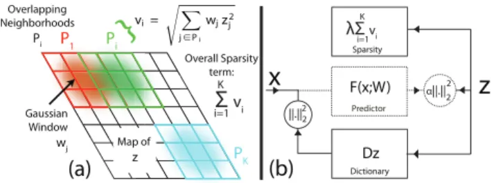
The overall idea [8] is to arrange thez’s into a 2D map (or some other topology) and then pool the squared coeffi-cients ofzacross overlapping windows. Then, the square of the the filter outputs within each sub-window are summed, and its square root is computed. More formally, let the map ofzcontainKoverlapping neighborhoodsPi. Within
each neighborhood i, we sum the squared coefficients zj
(weighted by a fixed Gaussian weighting function centered in the neighborhood) and then take the square root. This gives the activationvi =
q P
j∈Piwjz
2
j, wherewjare the
Gaussian weights. The overall sparsity penalty is the sum of each neighborhood’s activation:PK
i=1vi. Figure 1(a) il-lustrates this scheme. Thus, the overall objective function is now:
LI = 1
2||x− Dz||
2 2+λ
K X
i=1
s X
j∈Pi
||.||22
Dz
α||.||22
Dictionary
Predictor
Sparsity
K λΣ vi
i=1
x
F(x;W)z
P1 P1
Gaussian Window wj Overlapping Neighborhoods
Pi Pi
Map of z
{
K
Σ
vi
i=1
PK Overall Sparsity
term:
(a)
(b)
vi= j∈Pi
wjz2j
Figure 1. (a): The structure of the block-sparsity term which en-courages the basis functions inDto form a topographic map. See text for details. (b): Overall architecture of the loss function, as defined in Eqn. 4. In the generative model, we seek a feature vec-torzthat simultaneously approximate the inputxvia a dictionary
of basis functionsDand also minimize a sparsity term. Since per-forming the inference at run-time is slow, we train a prediction functionF(x;W)(dashed lines) that directly predicts the optimal zfrom the inputx. At run-time we use only the prediction function
to quickly computezfromx, from which the invariant featuresvi
can computed.
The modified sparsity term has a number of subtle effects on the nature ofzthat are not immediately obvious:
• The square root in the sum overi encourages sparse activations across neighborhoods since a few large ac-tivations will have lower overall cost than many small ones.
• Within each neighborhoodi, the coefficientszjare
en-couraged to be similar to one another due to thez2
jterm
(which prefers many small coefficients to a few large ones). This has the effect of encouraging similar basis functions inDto be spatially close in the 2D map. • As the neighborhoods overlap, these basis functions
will smoothly vary across the map, so that the coef-ficientszjin any given neighborhoodiwill be similar.
• If the size of the pooling regions is reduced to a single
zelement, then the sparsity term is equivalent to that of Eqn. 1.
The modified sparsity term means that by minimizing the loss functionLI in Eqn. 2 with respect to both the
co-efficientszand the dictionaryD, the system learns a set of basis functions inDthat are laid out in a topographic map on the 2D grid.
Since the nearby basis functions in the topographic map are similar, the coefficientszjwill be similar for a given
in-putx. This also means that if this input is perturbed slightly then the pooled response within a given neighborhood will be minimally affected, since a decrease in the response of one filter will be offset by an increased response in a nearby one. Hence, we can obtain a locally robust representation
by taking the pooled activationsvias features, rather thanz
as is traditionally done.
Since invariant representations encode similar patterns with the same representation, they can be made more com-pact. Put another way, this means that the dimensionality ofvcan be made lower than the dimensionality ofz with-out loss of useful information. This has the triple benefit of requiring less computation to extract the features from an image, requiring less memory to store them, and requiring less computation to exploit them.
The 2D map overzuses circular boundary conditions to ensure that the pooling wraps smoothly around at the edges of the map.
2.3. Code Prediction
The model proposed above is generative, thus at test-time for each input regionx, we will have to perform infer-ence by minimizing the energy functionLI of Eqn. 2 with
respect toz. However, this will be impractically slow for real-time applications where we wish to extract thousands of descriptors per image. We therefore propose to train a non-linear regressor that directly maps input patchesxinto sparse representationsz, from which the invariant features
vi can easily be computed. At test-time we only need to
presentxto the regression function which operates in feed-forward fashion to producez. No iterative optimization is needed.
For the regressor, we consider the following parametrized function:
F(x;W) =F(x;g, M, b) =gtanh(M x+b) (3) where M ∈ Rm×n is a filter matrix,b ∈ Rmis a vector
of biases,tanhis the hyperbolic tangent non-linearity, and
g∈ Rm×mis a diagonal matrix of gain coefficients
allow-ing the outputs ofF to compensate for the scaling of the input and the limited range of the hyperbolic tangent non-linearity. For convenience,Wis used to collectively denote the parameters of the predictor,W ={g, M, b}.
During training, the goal is to make the prediction of the regressor,F(x;W)as close as possible to the optimal set of coefficients: z∗
= arg minzLI in Eqn. (2). This
opti-mization can be carried out separately after the problem in Eqn. (2) has been solved. However, training becomes much faster by jointly optimizing theW and the set of basis func-tions D all together. This is achieved by adding another term to the loss function in Eqn. (2), which forces the rep-resentationzto be as close as possible to the feed-forward predictionF(x;W):
LIP =kx− Dzk22+λ K X
i=1
s X
j∈Pi
The overall structure of this loss function is depicted in Fig. 1(b).
2.4. Learning
The goal of learning is to find the optimal value of the ba-sis functionsD, as well as the value of the parameters in the regressorW, thus minimizingLIPin Eqn. 4. Learning
pro-ceeds by an on-line block coordinate gradient descent algo-rithm, alternating the following two steps for each training samplex.
1. Keeping the parametersW andDconstant, minimize LIP of Eqn. (4) with respect to z, starting from the
initial value provided by the regressorF(x;W). 2. Using the optimal value of the coefficientszprovided
by the previous step, update the parametersW andD by one step of stochastic gradient descent. The update is: U ← U −η∂LI P
∂U , whereU collectively denotes
{W,D}andηis the step size. The columns ofDare then re-scaled to unit norm.
We setα= 1for all experiments. We found that training the set of basis functionsDfirst, then subsequently training the regressor, yields similar performance in terms of recogni-tion accuracy. However, when the regressor is trained after-wards, the approximate representation is usually less sparse and the overall training time is considerably longer.
2.5. Evaluation
Once the parameters are learned, computing the invariant representationvcan be performed by a simple feed-forward propagation through the regressorF(x;W), and then prop-agatingz into v through vi =
q P
j∈Piwjz
2
j. Note that
no reconstruction of xusing the set of basis functions D is necessary any longer. An example of this feed forward recognition architecture is given in Fig. 6.
The addition of this feed-forward module for predicting
z, and hence,vis crucial to speeding up the run-time per-formance, since no optimization needs to be run after train-ing. Experiments reported in a technical report on the non-invariant version of Predictive Sparse Decomposition [9] show that the zproduced by this approximate representa-tion gives a slightly superior recognirepresenta-tion accuracy to thez
produced by optimizing ofLI.
Finally, other families of regressor functions were tested (using different kinds of thresholding non-linearities), but the one chosen here achieves similar performance while having the advantage of being very simple. In fact the fil-tersM learned by the prediction function closely match the basis functionsD used for reconstruction during training, having the same topographic layout.
Figure 2. Topographic map of feature detectors learned from nat-ural image patches of size 12x12 pixels by optimizingLI Pain
Eqn. 4. There are 400 filters that are organized in 6x6 neighbor-hoods. Adjacent neighborhoods overlap by 4 pixels both horizon-tally and vertically. Notice the smooth variation within a given neighborhood and also the circular boundary conditions.
4 8 12
4 8 12
0.25 0.125 16
16
Figure 3. Analysis of learned filters by fitting Gabor functions, each dot corresponding to a feature. Left: Center location of fitted Gabor. Right: Polar map showing the joint distribution of orienta-tion (azimuthally) and frequency (radially) of Gabor fit.
3. Experiments
In the following section, before exploring the properties of the invariant features obtained, we first study the topo-graphic map produced by our training scheme. First, we make an empirical evaluation of the invariance achieved by these representations under translations and rotations of the input image. Second, we assess the discriminative power of these invariant representations on recognition tasks in three different domains: (i) generic object categories using the Caltech 101 dataset; (ii) generic object categories from a dataset of very low resolution images and (iii) classification
Figure 4. Examples from the tiny images. We use grayscale images in our experiments.
of handwriting digits using the MNIST dataset. In these ex-periments we compare IPSD ’s learned representations with the SIFT descriptor [15] that is considered a state-of-the-art descriptor in computer vision. Finally, we examine the computational cost of computing IPSD features on an im-age.
3.1. Learning the Topographic Map
Fig. 2 shows a typical topographic map learned by the proposed method from natural image patches. Each tile shows a filter inDcorresponding to a particularzi. In the
example shown, the input images are patches of size 12x12 pixels, and there are 400 basis functions, and hence, 400 units zi arranged in a 20x20 lattice. The neighborhoods
over which the squared activities ofzi’s are pooled are 6x6
windows, and they overlap by 4 in both the vertical and the horizontal direction. The properties of these filters are ana-lyzed by fitting Gabor functions and are shown in Fig. 3.
By varying the way in which the neighborhoods are pooled, we can change the properties of the map. Larger neighborhoods make the filters in each pool increasingly similar. A larger overlap between windows makes the filters vary more smoothly across different pools. A large sparsity valueλmakes the feature detectors learn less localized pat-terns that look like those produced by k-means clustering because the input has to be reconstructed using a small num-ber of basis functions. On the other hand, a small sparsity value makes the feature detectors look like non-localized random filters because any random overcomplete basis set can produce good reconstructions (effectively, the first term in the loss of Eqn. 4 dominates).
The map in Fig. 2 has been produced with an intermedi-ate sparsity level ofλ= 3. The chosen parameter setting in-duces the learning algorithm to produce a smooth map with mostly localized edge detectors in different positions, ori-entations, and scales. These feature detectors are nicely or-ganized in such a way that neighboring units encode similar patterns. A unitvi, that connects to the sum of the squares of
unitszjin a pool is invariant because these units represent
similar features, and small distortions applied to the input, while slightly changing thezj’s within a pool, are likely to
leave the correspondingviunaffected.
While the sparsity level, the size of the pooling windows and their overlap should be set by cross-validation, in prac-tice we found that their exact values do not significantly
0 4 8 12 16
0 0.5 1 1.5
rotation 0 degrees
horizontal shift
Normalized MSE
0 4 8 12 16
0.2 0.4 0.6 0.8 1 1.2
rotation 25 degrees
horizontal shift Normalized MSE SIFT non rot. inv.
SIFT Our alg. non inv. Our alg. inv.
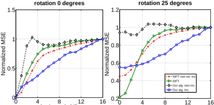
Figure 5. Mean squared error (MSE) between the representation of a patch and its transformed version. On the left panel, the formed patch is horizontally shifted. On the right panel, the trans-formed patch is first rotated by 25 degrees and then horizontally shifted. The curves are an average over 100 patches randomly picked from natural images. Since the patches are 16x16 pixels in size, a shift of 16 pixels generates a transformed patch that is quite uncorrelated to the original patch. Hence, the MSE has been normalized so that the MSE at 16 pixels is the same for all methods. This allows us to directly compare different feature ex-traction algorithms: non-orientation invariant SIFT, SIFT, IPSD trained to produce non-invariant representations (i.e. pools have size 1x1) [9], and IPSD trained to produce invariant representa-tions. All algorithms produce a feature vector with 128 dimen-sions. IPSD produces representations that are more invariant to transformations than the other approaches.
affect the kind of features learned. In other words, the al-gorithm is quite robust to the choice of these parameters, probably because of the many constraints enforced during learning.
3.2. Analyzing Invariance to Transformations
In this experiment we study the invariance properties of the learned representation under simple transformations. We have generated a dataset of 16x16 natural image patches under different translations and rotations. Each patch is pre-sented to the predictor function that produces a 128 dimen-sional descriptor (chosen to be the same size as SIFT) com-posed ofv’s. A representation can be considered locally in-variant if it does not change significantly under small trans-formations of the input. Indeed, this is what we observe in Fig. 5. We compare the mean squared difference be-tween the descriptor of the reference patch and the descrip-tor of the transformed version, averaged over many different image patches. The figure compares proposed descriptor against SIFT with a varying horizontal shift for 0 and 25 degrees initial rotation. Very similar results are found for vertical shifts and other rotation angles.
On the left panel, we can see that the mean squared error (MSE) between the representation of the original patch and its transformation increases linearly as we increase the hor-izontal shift. The MSE of IPSD representation is generally
√
√
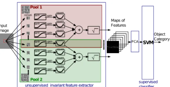
Figure 6. Diagram of the recognition system, which is composed of an invariant feature extractor that has been trained unsuper-vised, followed by a supervised linear SVM classifier. The fea-ture extractor process the input image through a set of filter banks, where the filters are organized in a two dimensional topographic map. The map defines pools of similar feature detectors whose ac-tivations are first non-linearly transformed by a hyperbolic tangent non-linearity, and then, multiplied by a gain. Invariant representa-tions are found by taking the square root of the sum of the squares of those units that belong to the same pool. The output of the fea-ture extractor is a set of feafea-ture maps that can be fed as input to the classifier. The filter banks and the set of gains is learned by the algorithm. Recognition is very fast, because it consists of a direct forward propagation through the system.
lower than the MSE produced by features that are computed using SIFT, a non-rotation invariant version of SIFT, and a non-invariant representation produced by the proposed method (that was trained with pools of size 1x1) [9]. A sim-ilar behavior is found when the patch is not only shifted, but also rotated. When the shift is small, SIFT has lower MSE, but as soon as the translation becomes large enough that the input pattern falls in a different internal sub-window, the MSE increases considerably. Instead learned represen-tations using IPSD seem to be quite robust to shifts, with an overall lower area under the curve. Note also that traditional sparse coding algorithms are prone to produce unstable rep-resentations under small distortions of the input. Because each input has to be encoded with a small number of basis functions, and because the basis functions are highly tuned in orientation and location, a small change in the input can produce drastic changes in the representation. This problem is partly alleviated by our approximate inference procedure that uses a smooth predictor function. However, this experi-ment shows that this representations is fairly unstable under small distortions, when compared to the invariant represen-tations produced by IPSD and SIFT.
3.3. Generic Object Recognition
We now use IPSD invariant features for object classifi-cation on the Caltech 101 dataset [5] of 102 generic object categories including background class. We use 30 training images per class and up to 30 test images per class. The images are randomly picked, and pre-processed in the
fol-lowing way: converted to gray-scale and down-sampled in such a way that the longest side is 151 pixels and then lo-cally normalized and zero padded to 143x143 pixels. The local normalization takes a 3x3 neighborhood around each pixel, subtracts the local mean, then divides the by the local standard deviation if it is greater than the standard deviation of the image. The latter step is a form of divisive normal-ization, proposed to model the contrast normalization in the retina [21].
We have trained IPSD on 50,000 16x16 patches ran-domly extracted from the pre-processed images. The topo-graphic map used has size 32x16, with the pooling neigh-borhoods being 6x6 and an overlap of 4 coefficients be-tween neighborhoods. Hence, there are a total of 512 units that are used in 128 pools to produce a 128-dimensional representation that can be compared to SIFT. After training IPSD in an unsupervised way, we use the predictor function to infer the representation of one whole image by: (i) run-ning the predictor function on 16x16 patches spaced by 4 pixels to produce 128 maps of features of size 32x32; (ii) the feature maps are locally normalized (neighborhood of 5x5) and low-pass filtered with a boxcar filter (5x5) to avoid aliasing; (iii) the maps are then projected along the leading 3060 principal components (equal to the number of train-ing samples), and (iv) a supervised linear SVM1 is trained
to recognize the object in each corresponding image. The overall scheme is shown in Fig. 6.
Table 1 reports the recognition results for this experi-ment. With a linear classifier similar to [21], IPSD features outperform SIFT and the model proposed by Serre and Pog-gio [25]. However, if rotation invariance is removed from SIFT its performance becomes comparable to IPSD .
We have also experimented with the more sophisticated Spatial Pyramid Matching (SPM) Kernel SVM classifier of Lazebnik et al. [11]. In this experiment, we again used the same IPSD architecture on 16x16 patches spaced by 3 pixels to produce 42x42x128 dimensional feature maps, followed by local normalization over a 9x9 neighborhood, yielding 128 dimensional features over a uniform 34x34 grid. Using SPM, IPSD features achieve 59.6% average accuracy per class. By decreasing the stepping stride to 1 pixel, thereby producing 120x120 feature maps, IPSD fea-tures achieve 65.5% accuracy as shown in Table 1. This is comparable to Lazebnik’s 64.6% accuracy on Caltech-101 (without background class) [11]. For comparison, our re-implementation of Lazebnik’s SIFT feature extractor, stepped by 4 pixels to produce 34x34 maps, yielded 65% average recognition rate.
With 128 invariant features, each descriptor takes around 4ms to compute from a 16x16 patch. Note that the evalua-tion time of each region is a linear funcevalua-tion of the number
1We have used LIBSVM package available at
Method Av. Accuracy/Class (%) local norm5×5+ boxcar5×5+ PCA3060+ linear SVM
IPSD (24x24) 50.9
SIFT (24x24) (non rot. inv.) 51.2
SIFT (24x24) (rot. inv.) 45.2
Serre et al. features [25] 47.1
local norm9×9+ Spatial Pyramid Match Kernel SVM
SIFT [11] 64.6
IPSD (34x34) 59.6
IPSD (56x56) 62.6
IPSD (120x120) 65.5
Table 1. Recognition accuracy on Caltech 101 dataset using a va-riety of different feature representations and two different classi-fiers. The PCA + linear SVM classifier is similar to [21], while the Spatial Pyramid Matching Kernel SVM classifier is that of [11]. IPSD is used to extract features with three different sampling step sizes over an input image to produce 34x34, 56x56 and 120x120 feature maps, where each feature is 128 dimensional to be compa-rable to SIFT. Local normalization is not applied on SIFT features when used with Spatial Pyramid Match Kernel SVM.
0 20 40 60 80 100 120 140
40 42 44 46 48 50 52
Number of Invariant Units
Recognition Accuracy (%)
Figure 7. The figure shows the recognition accuracy on Caltech 101 dataset as a function of the number of invariant units. Note that the performance improvement between 64 and 128 units is below 2%, suggesting that for certain applications the more com-pact descriptor might be preferable.
of features, thus this time can be further reduced if the num-ber of features is reduced. Fig. 7 shows how the recognition performance varies as the number of features is decreased.
3.4. Tiny Images classification
IPSD was compared to SIFT on another recognition task using the tiny images dataset [26]. This dataset was chosen as its extreme low-resolution provides a different setting to the Caltech 101 images. For simplicity, we selected 5 ani-mal nouns (abyssinian cat, angel shark, apatura iris (a type of butterfly), bilby (a type of marsupial), may beetle) and manually labeled 200 examples of each. 160 images of each class were used for training, with the remaining 40 held out for testing. All images are converted to grayscale. Both IPSD with 128 pooled units and SIFT were used to extract features over 16x16 regions, spaced every 4 pixels over the 32x32 images. The resulting 5 by 5 by 128 dimensional feature maps are used with a linear SVM. IPSD features achieve 54% and SIFT features achieve a comparable 53%.
Performance on Tiny Images Dataset
Method Accuracy (%)
IPSD (5x5) 54
SIFT (5x5) (non rot. inv.) 53 Performance on MNIST Dataset
Method Error Rate (%)
IPSD (5x5) 1.0
SIFT (5x5) (non rot. inv.) 1.5
Table 2. Results of recognition error rate on Tiny Images and MNIST datasets. In both setups, a 128 dimensional feature vector is obtained using either IPSD or SIFT over a regularly spaced 5x5 grid and afterwards a linear SVM is used for classification. For comparison purposes it is worth mentioning that a Gaussian SVM trained on MNIST images without any preprocessing achieves 1.4% error rate.
3.5. Handwriting Recognition
We use a very similar architecture to that used in the ex-periments above to train on the handwritten digits of the MNIST dataset [1]. This is a dataset of quasi-binary hand-written digits with 60,000 images in the training set, and 10,000 images in the test set. The algorithm was trained us-ing 16x16 windows extracted from the original 28x28 pixel images. For recognition, 128-dimensional feature vectors were extracted at 25 locations regularly spaced over a 5x5 grid. A linear SVM trained on these features yields an er-ror rate of 1.0%. When 25 SIFT feature vectors are used instead of IPSD features, the error rate increases to 1.5%. This demonstrates that, while SIFT seems well suited to natural images, IPSD produces features that can adept to the task at hand. In a similar experiment, a single 128-dimensional feature vector was extracted using IPSD and SIFT, and fed to a linear SVM. The error rate was 5.6% for IPSD , and 6.4% for SIFT.
4. Summary and Future Work
We presented an architecture and a learning algorithm that can learn locally-invariant feature descriptors. The ar-chitecture uses a bank of non-linear filters whose outputs are organized in a topographic fashion, followed by a pool-ing layer that imposes a sparsity criterion on blocks of fil-ter outputs located within small regions of the topographic map. As a result of learning, filters that are pooled together extract similar features, which results in spontaneous invari-ance of the pooled outputs to small distortions of the input. During training, the output of the non-linear filter bank is fed to a linear decoder that reconstructs the input patch. The filters and the linear decoder are simultaneously trained to minimize the reconstruction error, together with a sparsity criterion computed as the sum of the pooling units. After training, the linear decoder is discarded, and the pooling unit outputs are used as the invariant feature descriptor of the input patch. Computing the descriptor for a patch is very
fast and simple: it merely involves multiplying the patch by a filtering matrix, applying a scaled tanh function to the re-sults, and computing the square root of Gaussian-weighted sum-of-squares of filter outputs within each pool window.
Image classification experiments show that the descrip-tors thereby obtained give comparable performance to SIFT descriptors on tasks for which SIFT was specifically de-signed (such as Caltech 101), and better performance on tasks for which SIFT is not particularly well suited (MNIST, and Tiny Images).
While other models have learned locally invariant de-scriptors by explicitly building shift invariance using spa-tial pooling, our proposal is more general: it can learn local invariances to other transformations than just translations. Our results also show spontaneous local invariance to rota-tion. To our knowledge, this is the first time such invariant feature descriptors have been learned and tested in an image recognition context with competitive recognition rates.
A long-term goal of this work is to provide a general tool for learning feature descriptors in an unsupervised manner. Future work will involve “stacking” multiple stage of such feature extractors so as to learn multi-level hierarchies of increasingly global and invariant features.
5. Acknowledgments
We thank Karol Gregor, Y-Lan Boureau, Eero Simon-celli, and members of the CIfAR program Neural Computa-tion and Adaptive PercepComputa-tion for helpful discussions. This work was supported in part by ONR grant N00014-07-1-0535, NSF grant EFRI-0835878, and NSF IIS-0535166.
References
[1] http://yann.lecun.com/exdb/mnist/.
[2] M. Aharon, M. Elad, and A. Bruckstein. K-svd and its non-negative variant for dictionary design. volume 5914, 2005. [3] N. Dalal and B. Triggs. Histograms of oriented gradients for
human detection. In Proc. of Computer Vision and Pattern
Recognition, 2005.
[4] B. Efron, T. Hastie, I. Johnstone, and R. Tibshirani. Least angle regression, 2002,.
[5] L. Fei-Fei, R. Fergus, and P. Perona. Learning generative visual models from few training examples: An incremental bayesian approach tested on 101 object categories. In CVPR
Workshop, 2004.
[6] A. Hyvarinen and P. Hoyer. Emergence of phase- and shift-invariant features by decomposition of natural images into independent feature subspaces. Neural Comput, 12(7):1705– 1720, 2000 Jul.
[7] A. Hyvarinen and P. Hoyer. A two-layer sparse coding model learns simple and complex cell receptive fields and topog-raphy from natural images. Vision Research, 41(18):2413– 2423, 2001.
[8] A. Hyvarinen and U. Koster. Complex cell pooling and the statistics of natural images. Network, 18(2):81–100, 2007 Jun.
[9] K. Kavukcuoglu, M. Ranzato, and Y. LeCun. Fast infer-ence in sparse coding algorithms with applications to ob-ject recognition. Technical report, CBLL, Courant Institute, NYU, 2008. CBLL-TR-2008-12-01.
[10] T. Kohonen. Emergence of invariant-feature detectors in the adaptive-subspace self-organizing map. Biol. Cybern., 75:281–291, 1996.
[11] S. Lazebnik, C. Schmid, and J. Ponce. Beyond bags of features: Spatial pyramid matching for recognizing natural scene categories. In CVPR, pages 2169–2178. IEEE, June 2006.
[12] Y. LeCun, L. Bottou, Y. Bengio, and P. Haffner. Gradient-based learning applied to document recognition.
Proceed-ings of the IEEE, 86(11):2278–2324, November 1998.
[13] Y. LeCun, F.-J. Huang, and L. Bottou. Learning methods for generic object recognition with invariance to pose and lighting. In Proceedings of CVPR’04. IEEE Press, 2004. [14] H. Lee, A. Battle, R. Raina, and A. Ng. Efficient sparse
coding algorithms. In NIPS, 2006.
[15] D. Lowe. Distinctive image features from scale-invariant keypoints. IJCV, 2004.
[16] J. Mairal, F. Bach, J. Ponce, G. Sapiro, and A. Zisserman. Discriminative learned dictionaries for local image analysis. In CVPR, 2008.
[17] J. Murray and K. Kreutz-Delgado. Learning sparse overcom-plete codes for images. The Journal of VLSI Signal
Process-ing, 45:97–110, 2008.
[18] J. Mutch and D. Lowe. Multiclass object recognition with sparse, localized features. In CVPR, 2006.
[19] B. A. Olshausen and D. J. Field. Sparse coding with an over-complete basis set: a strategy employed by v1? Vision
Re-search, 37:3311–3325, 1997.
[20] S. Osindero, M. Welling, and G. E. Hinton. Topographic product models applied to natural scene statistics. Neural
Comput, 18(2):381–414, 2006 Feb.
[21] N. Pinto, D. D. Cox, and J. J. DiCarlo. Why is real-world vi-sual object recognition hard? PLoS Computational Biology, 4(1), 2008.
[22] M. Ranzato, F. Huang, Y. Boureau, and Y. LeCun. Unsuper-vised learning of invariant feature hierarchies with applica-tions to object recognition. In CVPR, 2007.
[23] M. Ranzato, C. Poultney, S. Chopra, and Y. LeCun. Effi-cient learning of sparse representations with an energy-based model. In NIPS, 2006.
[24] C. Rozell, D. Johnson, B. R.G., and B. Olshausen. Sparse coding via thresholding and local competition in neural cir-cuits. Neural Computation, 2008.
[25] T. Serre, L. Wolf, and T. Poggio. Object recognition with features inspired by visual cortex. In CVPR, 2005.
[26] A. Torralba, R. Fergus, and W. T. Freeman. 80 million tiny images: A large dataset for nonparametric object and scene recognition. IEEE PAMI, 30(11):1958–1970, 2008. [27] M. Yuan and Y. Lin. Model selection and estimation in
re-gression with grouped variables. Technical report, Univ. of Winsconsin, 2004.