Kevin Beyer, Jonathan Goldstein, Raghu Ramakrishnan, and Uri Shaft CS Dept., University of Wisconsin-Madison
1210 W. Dayton St., Madison, WI 53706 {beyer, jgoldst, raghu, uri}@cs.wisc.edu
Abstract. We explore the effect of dimensionality on the “nearest neigh-bor” problem. We show that under a broad set of conditions (much broader than independent and identically distributed dimensions), as di-mensionality increases, the distance to the nearest data point approaches the distance to the farthest data point. To provide a practical perspec-tive, we present empirical results on both real and synthetic data sets that demonstrate that this effect can occur for as few as 10-15 dimen-sions.
These results should not be interpreted to mean that high-dimensional indexing is never meaningful; we illustrate this point by identifying some high-dimensional workloads for which this effect does not occur. How-ever, our results do emphasize that the methodology used almost uni-versally in the database literature to evaluate high-dimensional indexing techniques is flawed, and should be modified. In particular, most such techniques proposed in the literature are not evaluated versus simple lin-ear scan, and are evaluated over workloads for which nlin-earest neighbor is not meaningful. Often, even the reported experiments, when analyzed carefully, show that linear scan would outperform the techniques being proposed on the workloads studied in high (10-15) dimensionality!
1
Introduction
In recent years, many researchers have focused on finding efficient solutions to the nearest neighbor (NN) problem, defined as follows: Given a collection of data points and a query point in an m-dimensional metric space, find the data point that is closest to the query point. Particular interest has centered on solving this problem in high dimensional spaces, which arise from tech-niques that approximate (e.g., see [24]) complex data—such as images (e.g. [15,28,29,21,29,23,25,18,3]), sequences (e.g. [2,1]), video (e.g. [15]), and shapes (e.g. [15,30,25,22])—with long “feature” vectors. Similarity queries are performed by taking a given complex object, approximating it with a high dimensional vec-tor to obtain the query point, and determining the data point closest to it in the underlying feature space.
This paper makes the following three contributions:
1) We show that under certain broad conditions (in terms of data and query dis-tributions, orworkload), as dimensionality increases, the distance to the nearest neighbor approaches the distance to the farthest neighbor. In other words, the Catriel Beeri, Peter Buneman (Eds.): ICDT’99, LNCS 1540, pp. 217–235, 1998.
c
contrastin distances to different data points becomes nonexistent. The conditions we have identified in which this happens are much broader than the indepen-dent and iindepen-dentically distributed (IID) dimensions assumption that other work assumes. Our result characterizes the problem itself, rather than specific algo-rithms that address the problem. In addition, our observations apply equally to the k-nearest neighbor variant of the problem. When one combines this result with the observation that most applications of high dimensional NN are heuris-tics for similarity in some domain (e.g. color histograms for image similarity), serious questions are raised as to the validity of many mappings of similarity problems to high dimensional NN problems. This problem can be further exac-erbated by techniques that find approximate nearest neighbors, which are used in some cases to improve performance.
2) To provide a practical perspective, we present empirical results based on syn-thetic distributions showing that the distinction between nearest and farthest neighbors may blur with as few as 15 dimensions. In addition, we performed experiments on data from a real image database that indicate that these dimen-sionality effects occur in practice (see [13]). Our observations suggest that high-dimensional feature vector representations for multimedia similarity search must be used with caution. In particular, one must check that the workload yields a clear separation between nearest and farthest neighbors for typical queries (e.g., through sampling). We also identify special workloads for which the concept of nearest neighbor continues to be meaningful in high dimensionality, to empha-size that our observations should notbe misinterpreted as saying that NN in high dimensionality is never meaningful.
3) We observe that the database literature on nearest neighbor processing tech-niques fails to compare new techtech-niques to linear scans. Furthermore, we can infer from their data that a linear scan almost always out-performs their tech-niques in high dimensionality on the examined data sets. This is unsurprising as the workloads used to evaluate these techniques are in the class of “badly behaving” workloads identified by our results; the proposed methods may well be effective for appropriately chosen workloads, but this is not examined in their performance evaluation.
In summary, our results suggest that more care be taken when thinking of nearest neighbor approaches and high dimensional indexing algorithms; we sup-plement our theoretical results with experimental data and a careful discussion.
2
On the Significance of “Nearest Neighbor”
The NN problem involves determining the point in a data set that is nearest to a given query point (see Figure 1). It is frequently used in Geographical Information Systems (GIS), where points are associated with some geographical location (e.g., cities). A typical NN query is: “What city is closest to my current location?”
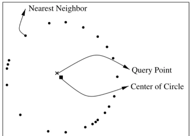
While it is natural to ask for the nearest neighbor, there is not always a meaningful answer. For instance, consider the scenario depicted in Figure 2.
Query Point Nearest Neighbor
Fig. 1. Query point and its nearest neighbor.
Query Point Center of Circle Nearest Neighbor
Fig. 2. Another query point and its nearest neighbor.
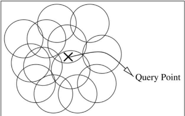
Even though there is a well-defined nearest neighbor, the difference in distance between the nearest neighbor and any other point in the data set is very small. Since the difference in distance is so small, the utility of the answer in solving concrete problems (e.g. minimizing travel cost) is very low. Furthermore, consider the scenario where the position of each point is thought to lie in some circle with high confidence (see Figure 3). Such a situation can come about either from numerical error in calculating the location, or “heuristic error”, which derives from the algorithm used to deduce the point (e.g. if a flat rather than a spherical map were used to determine distance). In this scenario, the determination of a nearest neighbor is impossible with any reasonable degree of confidence!
While the scenario depicted in Figure 2 is very contrived for a geographical database (and for any practical two dimensional application of NN), we show that it is the norm for a broad class of data distributions in high dimensionality. To establish this, we will examine the number of points that fall into a query sphere enlarged by some factor ε (see Figure 4). If few points fall into this enlarged sphere, it means that the data point nearest to the query point is separated from the rest of the data in a meaningful way. On the other hand, if
Query Point
Fig. 3. The data points are approximations. Each circle denotes a region where
the true data point is supposed to be.
(1+e)DMIN Q
DMIN DMAX
Fig. 4. Illustration of query region and enlarged region. (DMIN is the distance
to the nearest neighbor, and DMAX to the farthest data point.)
many (let alone most!) data points fall into this enlarged sphere, differentiating the “nearest neighbor” from these other data points is meaningless ifεis small. We use the notioninstabilityfor describing this phenomenon.
Definition 1 A nearest neighbor query isunstablefor a givenεif the distance
from the query point to most data points is less than (1 +ε)times the distance from the query point to its nearest neighbor.
We show that in many situations, for any fixedε >0, as dimensionality rises, the probability that a query is unstable converges to 1. Note that the points that fall in the enlarged query region are the valid answers to the approximate nearest neighbors problem (described in [6]).
3
NN in High-Dimensional Spaces
This section contains our formulation of the problem, our formal analysis of the effect of dimensionality on the meaning of the result, and some formal implica-tions of the result that enhance understanding of our primary result.
3.1 Notational Conventions
We use the following notation in the rest of the paper:
A vector: x
Probability of an event e: P[e].
Expectation of a random variable X: E[X].
Variance of a random variable X: var (X).
IID: Independent and identically distributed.
(This phrase is used with reference to the values assigned to a collection of random variables.)
X ∼F: A random variable X that takes on values following the distribution
F.
3.2 Some Results from Probability Theory
Definition 2 A sequence of random vectors (all vectors have the same arity)
A1,A2, . . . converges in probability to a constant vector c if for all ε > 0
the probability of A
m
being at most ε away from c converges to 1 asm→ ∞. In other words:∀ε >0, lim
m→∞P[kA
m
−ck ≤ε] = 1We denote this property by A
m
→pc. We also treat random variables that arenot vectors as vectors with arity 1.
Lemma 1 If B1, B2, . . . is a sequence of random variables with finite variance
andlimm→∞E[Bm] =b andlimm→∞var(Bm) = 0 thenBm→pb.
A version of Slutsky’s theorem Let A1,A2, . . . be random variables (or
vectors) and g be a continuous function. If A
m
→p c and g(c) is finite theng(A
m
)→pg(c).Corollary 1 (to Slutsky’s theorem) If X1, X2, . . . and Y1, Y2, . . . are
se-quences or random variables s.t.Xm→pa andYm→pb6= 0 thenXm/Ym→p
a/b.
3.3 Nearest Neighbor Formulation
Given a data set and a query point, we want to analyze how much the distance to the nearest neighbor differs from the distance to other data points. We do this by evaluating the number of points that are no farther away than a factor
ε larger than the distance between the query point and the NN, as illustrated in Figure 4. When examining this characteristic, we assume nothing about the structure of the distance calculation.
We will study this characteristic by examining the distribution of the dis-tance between query points and data points as some variablem changes. Note
that eventually, we will interpretmas dimensionality. However, nowhere in the following proof do we rely on that interpretation. One can view the proof as a convergence condition on a series of distributions (which we happen to call distance distributions) that provides us with a tool to talk formally about the “dimensionality curse”.
We now introduce several terms used in stating our result formally.
Definition 3:
m is the variable that our distance distributions may converge under (m ranges over all positive integers).
Fdata1, Fdata2, . . .is a sequence of data distributions.
Fquery1, Fquery2, . . . is a sequence of query distributions.
n is the (fixed) number of samples (data points) from each distribution.
∀m Pm,1, . . . , Pm,n are n independent data points per m such that Pm,i ∼
Fdatam.
Qm∼Fquerym is a query point chosen independently from allPm,i. 0< p <∞is a constant.
∀m, dm is a function that takes a data point from the domain of Fdatam and a
query point from the domain ofFquerymand returns a non-negative real number
as a result.
DMINm= min{dm(Pm,i, Qm)|1≤i≤n}.
DMAXm= max{dm(Pm,i, Qm)|1≤i≤n}.
3.4 Instability Result
Our main theoretical tool is presented below. In essence, it states that assuming the distance distribution behaves a certain way asmincreases, the difference in distance between the query point and all data points becomes negligible (i.e., the query becomes unstable). Future sections will show that the necessary behavior described in this section identifies a large class (larger than any other classes we are aware of for which the distance result is either known or can be readily inferred from known results) of workloads. More formally, we show:
Theorem 1 Under the conditions in Definition 3, if
lim m→∞var
(dm(Pm,1, Qm))p
E[(dm(Pm,1, Qm))p]
= 0 (1)
Then for every ε >0 lim
m→∞P[DMAXm≤(1 +ε)DMINm] = 1
Proof Letµm=E[(dm(Pm,i, Qm))p]. (Note that the value of this expectation
is independent ofisince allPm,i have the same distribution.) LetVm= (dm(Pm,1, Qm))p/µm.
Part 1: We’ll show thatVm→p1.
It follows that E[Vm] = 1 (because Vm is a random variable divided by its expectation.)
Trivially, limm→∞E[Vm] = 1.
The condition of the theorem (Equation 1) means that limm→∞var (Vm) = 0. This, combined with limm→∞E[Vm] = 1, enables us to use Lemma 1 to conclude that Vm→p1.
Part 2: We’ll show that ifVm→p1 then
lim
m→∞P[DMAXm≤(1 +ε)DMINm] = 1.
LetXm= (dm(Pm,1, Qm)/µm, . . . , dm(Pm,n, Qm)/µm) (a vector of arityn). Since each part of the vector Xm has the same distribution asVm, it follows that Xm→p(1, . . . ,1).
Since min and max are continuous functions we can conclude from Slutsky’s theorem that min(Xm)→pmin(1, . . . ,1) = 1, and similarly, max(Xm)→p1. Using Corollary 1 on max(Xm) and min(Xm) we get
max(Xm) min(Xm) →p
1 1 = 1
Note that DMINm=µmmin(Xm) and DMAXm=µmmax(Xm). So, DMAXm
DMINm =
µmmax(Xm)
µmmin(Xm) =
max(Xm) min(Xm) Therefore,
DMAXm DMINm →p1
By definition of convergence in probability we have that for allε >0, lim
m→∞P
DMAXm DMINm −1
≤ε
= 1 Also,
P[DMAXm≤(1 +ε)DMINm] =P
DMAXm DMINm −1≤ε
=PDMAXm
DMINm −1
≤ε
(P[DMAXm≥DMINm] = 1 so the absolute value in the last term has no effect.) Thus,
lim
m→∞P[DMAXm≤(1 +ε)DMINm] = limm→∞P
DMAXm DMINm −1
≤ε
= 1
In summary, the above theorem says that if the precondition holds (i.e., if the distance distribution behaves a certain way as mincreases), all points converge
to the same distance from the query point. Thus, under these conditions, the concept of nearest neighbor is no longer meaningful.
We may be able to use this result by directly showing thatVm→p1 and using part 2 of the proof. (For example, for IID distributions,Vm→p1 follows readily from the Weak Law of Large Numbers.) Later sections demonstrate that our result provides us with a handy tool for discussing scenarios resistant to analysis using law of large numbers arguments. From a more practical standpoint, there are two issues that must be addressed to determine the theorem’s impact:
– How restrictive is the condition lim m→∞var
(dm(Pm,1, Qm))p
E[(dm(Pm,1, Qm))p]
=
= lim m→∞
var ((dm(Pm,1, Qm))p) (E[(dm(Pm,1, Qm))p])
2 = 0 (2)
which is necessary for our results to hold? In other words, it says that as we increasem and examine the resulting distribution of distances between queries and data, the variance of the distance distribution scaled by the overall magnitude of the distance converges to 0. To provide a better under-standing of the restrictiveness of this condition, Sections 3.5 and 4 discuss scenarios that do and do not satisfy it.
– For situations in which the condition is satisfied, at what rate do distances be-tween points become indistinct as dimensionality increases? In other words, at what dimensionality does the concept of “nearest neighbor” become mean-ingless? This issue is more difficult to tackle analytically. We therefore per-formed a set of simulations that examine the relationship betweenmand the ratio of minimum and maximum distances with respect to the query point. The results of these simulations are presented in Section 5 and in [13].
3.5 Application of Our Theoretical Result
This section analyses the applicability of Theorem 1 in formally defined situ-ations. This is done by determining, for each scenario, whether the condition in Equation 2 is satisfied. Due to space considerations, we do not give a proof whether the condition in Equation 2 is satisfied or not. [13] contains a full anal-ysis of each example.
All of these scenarios define a workload and use anLp distance metric over multidimensional query and data points with dimensionalitym. (This makes the data and query points vectors with aritym.) It is important to notice that this is the first section to assign a particular meaning todm(as anLpdistance metric),
p(as the parameter toLp), andm(as dimensionality). Theorem 1 did not make use of these particular meanings.
We explore some scenarios that satisfy Equation 2 and some that do not. We start with basic IID assumptions and then relax these assumptions in various ways. We start with two “sanity checks”: we show that distances converge with
IID dimensions (Example 1), and we show that Equation 2 is not satisfied when the data and queries fall on a line (Example 2). We then discuss examples involv-ing correlated attributes and differinvolv-ing variance between dimensions, to illustrate scenarios where the Weak Law of Large Numbers cannot be applied (Examples 3, 4, and 5).
Example 1 IID Dimensions with Query and Data Independence.
Assume the following:
– The data distribution and query distribution are IID in all dimensions.
– All the appropriate moments are finite (i.e., up to thed2pe’th moment).
– The query point is chosen independently of the data points.
The conditions of Theorem 1 are satisfied under these assumptions. While this result is not original, it is a nice “sanity check.” (In this very special case we can prove Part 1 of Theorem 1 by using the weak law of large numbers. How-ever, this is not true in general.) The assumptions of this example are by no means necessary for Theorem 1 to be applicable. Throughout this section, there are examples of workloads which cannot be discussed using the Weak Law of Large Numbers. While there are innumerable slightly stronger versions of the Weak Law of Large Numbers, Example 5 contains an example which meets our condition, and for which the Weak Law of Large Numbers is inapplicable.
Example 2 Identical Dimensions with no Independence.
We use the same notation as in the previous example. In contrast to the previous case, consider the situation where all dimensions of both the query point and the data points follow identical distributions, but are completely dependent (i.e., value for dimension 1 = value for dimension 2 =. . .). Conceptually, the result is a set of data points and a query point on a diagonal line. No matter how many dimensions are added, the underlying query can actually be converted to a one-dimensional nearest neighbor problem. It is not surprising to find that the condition of Theorem 1 is not satisfied.
Example 3 Unique Dimensions with Correlation Between All Dimensions.
In this example, we intentionally break many assumptions underlying the IID case. Not only is every dimension unique, butall dimensions are correlated with all other dimensions and the variance of each additional dimension increases. The following is a description of the problem.
We generate anmdimensional data point (or query point)Xm= (X1,. . ., Xm) as follows:
– First we take independent random variables
U1, . . . , Umsuch thatUi∼Uniform(0,
√
i).
– We defineX1=U1.
– For all 2≤i≤mdefineXi=Ui+ (Xi−1/2). The condition of Theorem 1 is satisfied.
Example 4 Variance Converging to 0.
This example illustrates that there are workloads that meet the preconditions of Theorem 1, even though the variance of the distance in each added dimension converges to 0. One would expect that only some finite number of the earlier dimensions would dominate the distance. Again, this is not the case.
Suppose we choose a pointXm= (X1, . . . , Xm) such that theXi’s are inde-pendent and Xi∼N(0,1/i). Then the condition of Theorem 1 is satisfied.
Example 5 Marginal Data and Query Distributions Change with
Dimension-ality.
In this example, the marginal distributions of data and queries change with di-mensionality. Thus, the distance distribution as dimensionality increases cannot be described as the distance in a lower dimensionality plus some new component from the new dimension. As a result, the weak law of large numbers, which im-plicitly is about sums of increasing size, cannot provide insight into the behavior of this scenario. The distance distributions must be treated, as our technique suggests, as a series of random variables whose variance and expectation can be calculated and examined in terms of dimensionality.
Let themdimensional data spaceSm be the boundary of anmdimensional unit hyper-cube. (i.e., Sm= [0,1]m−(0,1)m). In addition, let the distribution of data points be uniform overSm. In other words, every point inSmhas equal probability of being sampled as a data point. Lastly, the distribution of query points is identical to the distribution of data points.
Note that the dimensions are not independent. Even in this case, the condi-tion of Theorem 1 is satisfied.
4
Meaningful Applications of High Dimensional NN
In this section, we place Theorem 1 in perspective, and observe that it should
not be interpreted to mean that high-dimensional NN is never meaningful. We do this by identifying scenarios that arise in practice and that are likely to have good separation between nearest and farthest neighbors.
4.1 Classification and Approximate Matching
To begin with, exact match and approximate match queries can be reasonable. For instance, if there is dependence between the query point and the data points such that there exists some data point that matches the query point exactly, then DMINm = 0. Thus, assuming that most of the data points aren’t duplicates, a meaningful answer can be determined. Furthermore, if the problem statement is relaxed to require that the query point be within some small distance of a data point (instead of being required to be identical to a data point), we can still call the query meaningful. Note, however, that staying within the same small distance becomes more and more difficult asmincreases since we are adding terms to the
Query Point
Nearest Cluster
Fig. 5. Nearest neighbor query in clustered data.
sum in the distance metric. For this version of the problem to remain meaningful as dimensionality increases, the query point must be increasingly closer to some data point.
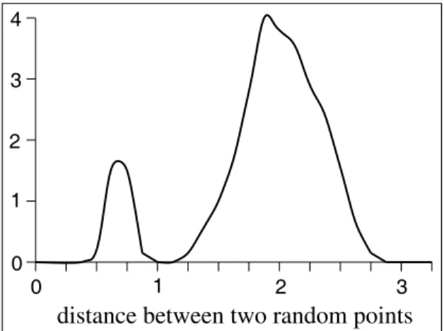
We can generalize the situation further as follows: The data consists of a set of randomly chosen points together with additional points distributed in clusters of some radius δ around one or more of the original points, and the query is required to fall within one of the data clusters (see Figure 5). This situation is the perfectly realized classification problem, where data naturally falls into discrete classes or clusters in some potentially high dimensional feature space. Figure 6 depicts a typical distance distribution in such a scenario. There is a cluster (the one into which the query point falls) that is closer than the others, which are all, more or less, indistinguishable in distance. Indeed, the proper response to such a query is to return all points within the closest cluster, not just the nearest point (which quickly becomes meaningless compared to other points in the cluster as dimensionality increases).
Observe however, that if we don’t guarantee that the query point falls within some cluster, then the cluster from which the nearest neighbor is chosen is subject to the same meaningfulness limitations as the choice of nearest neighbor in the original version of the problem; Theorem 1 then applies to the choice of the “nearest cluster”.
4.2 Implicitly Low Dimensionality
Another possible scenario where high dimensional nearest neighbor queries are meaningful occurs when the underlying dimensionality of the data is much lower than the actual dimensionality. There has been recent work on identifying these situations (e.g. [17,8,16]) and determining the useful dimensions (e.g. [20], which uses principal component analysis to identify meaningful dimensions). Of course, these techniques are only useful if NN in the underlying dimensionality is mean-ingful.
0 1 2 3 4
3 2
0
distance between two random points
1
Fig. 6. Probability density function of distance between random clustered data
and query points.
5
Experimental Studies of NN
Theorem 1 only tells us what happens when we take the dimensionality to in-finity. In practice, at what dimensionality do we anticipate nearest neighbors to become unstable? In other words, Theorem 1 describes some convergence but does not tell us the rate of convergence. We addressed this issue through em-pirical studies. Due to lack of space, we present only three synthetic workloads and one real data set. [13] includes additional synthetic workloads along with workloads over a second real data set.
We ran experiments with one IID uniform(0,1) workload and two different correlated workloads. Figure 7 shows the average DMAXm/DMINm as dimen-sionality increases of 1000 query points on synthetic data sets of one million tuples. The workload for the “recursive” line (described in Example 3) has correlation between every pair of dimensions and every new dimension has a larger variance. The “two degrees of freedom” workload generates query and data points on a two dimensional plane, and was generated as follows:
– Leta1, a2, . . .andb1, b2, . . .be constants in (-1,1). – LetU1, U2 be independent uniform(0,1).
– For all 1≤i≤mletXi=aiU1+biU2.
This last workload does not satisfy Equation 2. Figure 7 shows that the “two degrees of freedom” workload behaves similarly to the (one or) two dimensional uniform workload, regardless of the dimensionality. However, the recursive work-load (as predicted by our theorem) was affected by dimensionality. More in-terestingly, even with all the correlation and changing variances, the recursive workload behaved almost the same as the IID uniform case!
This graph demonstrates that our geometric intuition for nearest neighbor, which is based on one, two, and three dimensions, fails us at an alarming rate as
1
10
100
1000
10000
100000
1e+06
1e+07
1e+08
0
10 20 30 40 50 60 70 80 90 100
DMAX / DMIN (LOG SCALE)
dimensions (m)
two degrees of freedom
recursive
uniform
Fig. 7. Correlated distributions, one million tuples.
dimensionality increases. The distinction between nearest and farthest points, even at ten dimensions, is a tiny fraction of what it is in one, two, or three dimensions. For one dimension, DMAXm/DMINmfor “uniform” is on the order of 107, providing plenty of contrast between the nearest object and the farthest object. At 10 dimensions, this contrast is already reduced by 6 orders of mag-nitude! By 20 dimensions, the farthest point is only 4 times the distance to the closest point. These empirical results suggest that NN can become unstable with as few as 10-20 dimensions.
Figure 8 shows results for experiments done on a real data set. The data set was a 256 dimensional color histogram data set (one tuple per image) that was reduced to 64 dimensions by principal components analysis. There were approximately 13,500 tuples in the data set. We examine k-NN rather than NN because this is the traditional application of image databases.
To determine the quality of answers for NN queries, we examined the per-centage of queries in which at least half the data points were within some factor of the nearest neighbor. Examine the graph atmedian distance/k distance = 3. The graph says that fork= 1 (normal NN problem), 15% of the queries had at least half the data within a factor of 3 of the distance to the NN. Fork = 10, 50% of the queries had at least half the data within a factor of 3 of the distance to the 10th nearest neighbor. It is easy to see that the effect of changing k on the quality of the answer is most significant for small values ofk.
0
0.2
0.4
0.6
0.8
1
1
2
3
4
5
6
7
8
9
10
cumulative percent of queries
median distance / k distance
k = 1
k = 10
k = 100
k = 1000
Fig. 8. 64-D color histogram data.
Does this data set provide meaningful answers to the 1-NN problem? the 10-NN problem? the 100-10-NN problem? Perhaps, but keep in mind that the data set was derived using a heuristic that approximates image similarity. Furthermore, the nearest neighbor contrast is much lower than our intuition suggests (i.e., 2 or 3 dimensions). A careful evaluation of the relevance of the results is definitely called for.
6
Analyzing the Performance of a NN Processing
Technique
In this section, we discuss the ramifications of our results when evaluating tech-niques to solve the NN problem; in particular, many high-dimensional indexing techniques have been motivated by the NN problem. An important point that we make is that all future performance evaluations of high dimensional NN queries must include a comparison to linear scans as a sanity check.
First, our results indicate that while there exist situations in which high dimensional nearest neighbor queries are meaningful, they are very specific in nature and are quite different from the “independent dimensions” basis that most studies in the literature (e.g., [31,19,14,10,11]) use to evaluate techniques in a controlled manner. In the future, these NN technique evaluations should focus on those situations in which the results are meaningful. For instance, answers
are meaningful when the data consists of small, well-formed clusters, and the query is guaranteed to land in or very near one of these clusters.
In terms of comparisons between NN techniques, most papers do not compare against the trivial linear scan algorithm. Given our results, which argue that in many cases, as dimensionality increases, all data becomes equidistant to all other data, it is not surprising that in as few as 10 dimensions, linear scan handily beats these complicated indexing structures. 1 We give a detailed and formal discussion of this phenomenon in [27].
For instance, the performance study of the parallel solution to the k-nearest neighbors problem presented in [10] indicates that their solution scales more poorly than a parallel scan of the data, and never beats a parallel scan in any of the presented data.
[31] provides us with information on the performance of both the SS tree and the R* tree in finding the 20 nearest neighbors. Conservatively assuming that linear scans cost 15% of a random examination of the data pages, linear scan outperforms both the SS tree and the R* tree at 10 dimensions in all cases. In [19], linear scan vastly outperforms the SR tree in all cases in this paper for the 16 dimensional synthetic data set. For a 16 dimensional real data set, the SR tree performs similarly to linear scan in a few experiments, but is usually beaten by linear scan. In [14], performance numbers are presented for NN queries where bounds are imposed on the radius used to find the NN. While the performance in high dimensionality looks good in some cases, in trying to duplicate their results we found that the radius was such that few, if any, queries returned an answer. While performance of these structures in high dimensionality looks very poor, it is important to keep in mind that all the reported performance studies exam-ined situations in which the distance between the query point and the nearest neighbor differed little from the distance to other data points. Ideally, they should be evaluated for meaningful workloads. These workloads include low dimensional spaces and clustered data/queries as described in Section 4. Some of the existing structures may, in fact, work well in appropriate situations.
7
Related Work
7.1 The Curse of Dimensionality
The term dimensionality curse is often used as a vague indication that high dimensionality causes problems in some situations. The term was first used by Bellman in 1961 [7] for combinatorial estimation of multivariate functions. An example from statistics: in [26] it is used to note that multivariate density esti-mation is very problematic in high dimensions.
1 Linear scan of a set of sequentially arranged disk pages is much faster than unordered retrieval of the same pages; so much so that secondary indexes are ignored by query optimizers unless the query is estimated to fetch less than 10% of the data pages. Fetching a large number of data pages through a multi-dimensional index usually results in unordered retrieval.
In the area ofthe nearest neighbors problem it is used for indicating that a query processing technique performs worse as the dimensionality increases. In [11,5] it was observed that in some high dimensional cases, the estimate of NN query cost (using some index structure) can be very poor if “boundary effects” are not taken into account. The boundary effect is that the query region (i.e., a sphere whose center is the query point) is mainly outside the hyper-cubic data space. When one does not take into account the boundary effect, the query cost estimate can be much higher than the actual cost. The termdimensionality curse
was also used to describe this phenomenon.
In this paper, we discuss the meaning of the nearest neighbor query and not how to process such a query. Therefore, the termdimensionality curse(as used by the NN research community) is only relevant to Section 6, and not to the main results in this paper.
7.2 Computational Geometry
The nearest neighbor problem has been studied in computational geometry (e.g., [4,5,6,9,12]). However, the usual approach is to take the number of dimensions as a constant and find algorithms that behave well when the number of points is large enough. They observe that the problem is hard and define the approximate nearest neighbor problem as a weaker problem. In [6] there is an algorithm that retrieves an approximate nearest neighbor inO(logn) time for any data set. In [9] there is an algorithm that retrieves the true nearest neighbor in constant expected time under the IID dimensions assumption. However, the constants for those algorithms are exponential in dimensionality. In [6] they recommend not to use the algorithm in more than 12 dimensions. It is impractical to use the algorithm in [9] when the number of points is much lower than exponential in the number of dimensions.
7.3 Fractal Dimensions
In [17,8,16] it was suggested that real data sets usually have fractal properties (self-similarity, in particular) and that fractal dimensionality is a good tool in determining the performance of queries over the data set.
The following example illustrates that the fractal dimensionality of the data space from which we sample the data points may not always be a good indicator for the utility of nearest neighbor queries. Suppose the data points are sampled uniformly from the vertices of the unit hypercube. The data space is 2mpoints (in m dimensions), so its fractal dimensionality is 0. However, this situation is one of the worst cases for nearest neighbor queries. (This is actually the IID Bernoulli(1/2) which is even worse than IID uniform.) When the number of data points in this scenario is close to 2m, nearest neighbor queries become stable, but this is impractical for largem.
However, are there real data sets for which the (estimated) fractal dimension-ality is low, yet there is no separation between nearest and farthest neighbors? This is an intriguing question that we intend to explore in future work.
We used the technique described in [8] on two real data sets (described in [13]). However, the fractal dimensionality of those data sets could not be esti-mated (when we divided the space once in each dimension, most of the data points occupied different cells). We used the same technique on an artificial 100 dimensional data set that has known fractal dimensionality 2 and about the same number of points as the real data sets (generated like the “two degrees of freedom” workload in Section 5, but with less data). The estimate we got for the fractal dimensionality is 1.6 (which is a good estimate). Our conclusion is that the real data sets we used are inherently high dimensional; another possible explanation is that they do not exhibit fractal behavior.
8
Conclusions
In this paper, we studied the effect of dimensionality on NN queries. In particular, we identified a broad class of workloads for which the difference in distance between the nearest neighbor and other points in the data set becomes negligible. This class of distributions includes distributions typically used to evaluate NN processing techniques. Many applications use NN as a heuristic (e.g., feature vectors that describe images). In such cases, query instability is an indication of a meaningless query. This problem is worsened by the use of techniques that provide an approximate nearest neighbor to improve performance.
To find the dimensionality at which NN breaks down, we performed exten-sive simulations. The results indicated that the distinction in distance decreases fastest in the first 20 dimensions, quickly reaching a point where the difference in distance between a query point and the nearest and farthest data points drops below a factor of four. In addition to simulated workloads, we also examined two real data sets that behaved similarly (see [13]).
In addition to providing intuition and examples of distributions in that class, we also discussed situations in which NN queries do not break down in high dimensionality. In particular, the ideal data sets and workloads for classifica-tion/clustering algorithms seem reasonable in high dimensionality. However, if the scenario is deviated from (for instance, if the query point does not lie in a cluster), the queries become meaningless.
The practical ramifications of this paper are for the following two scenarios:
Evaluating a NN workload. Make sure that the distance distribution
(be-tween a random query point and a random data point) allows for enough contrast for your application. If the distance to the nearest neighbor is not much different from the average distance, the nearest neighbor may not be useful (or the most “similar”).
Evaluating a NN processing technique. When evaluating a NN processing
technique, test it on meaningful workloads. Examples for such workloads are given in Section 4. In addition, the evaluation of the technique for a particular workload should take into account any approximations that the technique uses to improve performance. Also, one should ensure that a new processing technique outperforms the most trivial solutions (e.g., sequential scan).
9
Acknowledgements
This work was partially supported by a “David and Lucile Packard Foundation Fellowship in Science and Engineering”, a “Presidential Young Investigator” award, NASA research grant NAGW-3921, ORD contract 144-ET33, and NSF grant 144-GN62.
We would also like to thank Prof. Robert Meyer for his time and valuable feedback. We would like to thank Prof. Rajeev Motwani for his helpful comments.
References
1. Agrawal, R., Faloutsos, C., Swami, A.: Efficient Similarity Search in Sequence Databases. In Proc. 4th Inter. Conf. on FODO (1993) 69–84
2. Altschul, S.F., Gish, W., Miller, W., Myers, E., Lipman, D.J.: Basic Local Align-ment Search Tool. In Journal of Molecular Biology, Vol. 215 (1990) 403–410 3. Ang, Y.H., Li, Z., Ong, S.H.: Image retrieval based on multidimensional feature
properties. In SPIE, Vol. 2420 (1995) 47–57
4. Arya, S.: Nearest Neighbor Searching and Applications. Ph.D. thesis, Univ. of Maryland at College Park (1995)
5. Arya, S., Mount, D.M., Narayan, O.: Accounting for Boundary Effects in Nearest Neighbors Searching. In Proc. 11th ACM Symposium on Computational Geometry (1995) 336–344
6. Arya, S., Mount, D.M., Netanyahu, N.S., Silverman, R., Wu, A.: An Optimal Algorithm for Nearest Neighbor Searching. In Proc. 5th ACM SIAM Symposium on Discrete Algorithms (1994) 573–582
7. Bellman, R.E.: Adaptive Control Processes. Princeton University Press (1961) 8. Belussi, A., Faloutsos, C.: Estimating the Selectivity of Spatial Queries Using the
‘Correlation’ Fractal Dimension. In Proc. VLDB (1995) 299–310
9. Bentley, J.L., Weide, B.W., Yao, A.C.: Optimal Expected-time Algorithms for Closest Point Problem”, In ACM Transactions on Mathematical Software, Vol. 6, No. 4 (1980) 563–580
10. Berchtold, S., B¨ohm, C., Braunm¨uller, B., Keim, D.A., Kriegel, H.-P.: Fast Parallel Similarity Search in Multimedia Databases. In Proc. ACM SIGMOD Int. Conf. on Management of Data (1997) 1–12
11. Berchtold, S., B¨ohm, C., B., Keim, D.A., Kriegel, H.-P.: A Cost Model for Nearest Neighbor Search in High-Dimensional Data Space. In Proc. 16th ACM SIGACT-SIGMOD-SIGART Symposium on PODS (1997) 78–86
12. Bern, M.: Approximate Closest Point Queries in High Dimensions. In Information Processing Letters, Vol. 45 (1993) 95–99
13. Beyer, K., Goldstein, J., Ramakrishnan, R., Shaft, U.: When Is Nearest Neighbors Meaningful? Technical Report No. TR1377, Computer Sciences Dept., Univ. of Wisconsin-Madison, June 1998
14. Bozkaya, T., Ozsoyoglu, M.: Distance-Based Indexing for High-Dimensional Metric Spaces. In Proc. 16th ACM SIGACT-SIGMOD-SIGART Symposium on PODS (1997) 357–368
15. Faloutsos, C., et al: Efficient and Effective Querying by Image Content. In Journal of Intelligent Information Systems, Vol. 3, No. 3 (1994) 231–262
16. Faloutsos, C., Gaede, V.: Analysis of n-Dimensional Quadtrees Using the Housdorff Fractal Dimension. In Proc. ACM SIGMOD Int. Conf. of the Management of Data (1996)
17. Faloutsos, C., Kamel, I.: Beyond Uniformity and Independence: Analysis of R-trees Using the Concept of Fractal Dimension. In Proc. 13th ACM SIGACT-SIGMOD-SIGART Symposium on PODS (1994) 4–13
18. Fayyad, U.M., Smyth, P.: Automated Analysis and Exploration of Image Databases: Results, Progress and Challenges. In Journal of intelligent information systems, Vol. 4, No. 1 (1995) 7–25
19. Katayama, N., Satoh, S.: The SR-tree: An Index Structure for High-Dimensional Nearest Neighbor Queries. In Proc. 16th ACM SIGACT-SIGMOD-SIGART Sym-posium on PODS (1997) 369–380
20. Lin, K.-I., Jagadish, H.V., Faloutsos, C.: The TV-Tree: An Index Structure for High-Dimensional Data. In VLDB Journal, Vol. 3, No. 4 (1994) 517–542
21. Manjunath, B.S., Ma, W.Y.: Texture Features for Browsing and Retrieval of Image Data. In IEEE Trans. on Pattern Analysis and Machine Learning, Vol. 18, No. 8 (1996) 837–842
22. Mehrotra, R., Gary, J.E.: Feature-Based Retrieval of Similar Shapes. In 9th Data Engineering Conference (1992) 108–115
23. Murase, H., Nayar, S.K.: Visual Learning and Recognition of 3D Objects from Appearance. In Int. J. of Computer Vision, Vol. 14, No. 1 (1995) 5–24
24. Nene, S.A., Nayar, S.K.: A Simple Algorithm for Nearest Neighbor Search in High Dimensions. In IEEE Trans. on Pattern Analysis and Machine Learning, Vol. 18, No. 8 (1996) 989–1003
25. Pentland, A., Picard, R.W., Scalroff, S.: Photobook: Tools for Content Based Ma-nipulation of Image Databases. In SPIE Vol. 2185 (1994) 34–47
26. Scott, D.W.: Multivariate Density Estimation. Wiley Interscience, Chapter 2 (1992)
27. Shaft, U., Goldstein, J., Beyer, K.: Nearest Neighbors Query Performance for Un-stable Distributions. Technical Report No. TR1388, Computer Sciences Dept., Univ. of Wisconsin-Madison, October 1998
28. Swain, M.J., Ballard D.H.: Color Indexing. In Inter. Journal of Computer Vision, Vol. 7, No. 1 (1991) 11-32
29. Swets, D.L., Weng, J.: Using Discriminant Eigenfeatures for Image Retrieval. In IEEE Trans. on Pattern Analysis and Machine Learning, Vol. 18, No. 8 (1996) 831–836
30. Taubin, G., Cooper, D.B.: Recognition and Positioning of Rigid Objects Using Algebraic Moment Invariants. In SPIE, Vol. 1570 (1991) 318–327
31. White, D.A., Jain, R.: Similarity Indexing with the SS-Tree. In ICDE (1996) 516– 523