Toby Ord
Department of Philosophy*
The University of Melbourne [email protected]
Abstract:
In this report I provide an introduction to the burgeoning field of hypercomputation – the study of machines that can compute more than Turing machines. I take an extensive survey of many of the key concepts in the field, tying together the disparate ideas and presenting them in a structure which allows comparisons of the many approaches and results. To this I add several new results and draw out some interesting consequences of hypercomputation for several different disciplines.
I begin with a succinct introduction to the classical theory of computation and its place amongst some of the negative results of the 20th Century. I then explain how the Church-Turing Thesis is commonly
misunderstood and present new theses which better describe the possible limits on computability. Following this, I introduce ten different hypermachines (including three of my own) and discuss in some depth the manners in which they attain their power and the physical plausibility of each method. I then compare the powers of the different models using a device from recursion theory. Finally, I examine the implications of hypercomputation to mathematics, physics, computer science and philosophy. Perhaps the most important of these implications is that the negative mathematical results of Gödel, Turing and Chaitin are each dependent upon the nature of physics. This both weakens these results and provides strong links between mathematics and physics. I conclude that hypercomputation is of serious academic interest within many disciplines, opening new possibilities that were previously ignored because of long held misconceptions about the limits of computation.
* The majority of this report was written as an Honours thesis at the Department of Computer Science in the University of Melbourne. This work was supervised by Harald Søndergaard.
In writing this report, I am indebted to four people. Jack Copeland, for introducing me to hypercomputation and taking my new ideas seriously. Harald Søndergaard, for allowing me the chance to do my Honours thesis on such a fascinating topic and then keeping me focused when I inevitably tried to take on too much. Peter Eckersley, for his ever enthusiastic conversations on the limits of logical thought. And finally, Bernadette Young, for her kindness and support when things looked impossible.
It has long been assumed that the Turing machine computes all the functions that are computable in any reasonable sense. It is therefore assumed to be a sufficient model for computability. What then, is one to make of the slow trickle of papers that discuss models which can compute more than the Turing machine? It is perhaps tempting to dismiss such theorising as idle speculation alike to the more fanciful areas of pure mathematics, in which models and abstractions are studied for their own sake with little regard to any real world implications.
This would be a great mistake. The study of more powerful models of computation is of considerable importance, with many far-reaching implications in computer science, mathematics, physics and philosophy. Rarely, if ever, has such an important physical claim about the limits of the universe been so widely accepted from such a weak basis of evidence. The inability of some of the best minds of the century to develop ways in which we could build machines with more computational power than Turing machines is not good evidence that this is impossible. At best, it is reason to consider the problem to be very difficult and likely to require a radically new technique or even new developments in physics.
However, we should not even go this far. A variety of theoretical models for such hypercomputation have been presented over the past century. They have, however, often been presented in rather theoretical contexts, which explains the lack of serious work on exploring the physical realisability of these models. Indeed, from what work has been done, there have recently been several serious reports about how quantum mechanics and relativity may be used to harness hypercomputation.
In many ways, the present theory of computation is in a similar position to that of geometry in the 18th
and 19th Centuries. In 1817 one of the most eminent mathematicians, Carl Friedrich Gauss, became
convinced that the fifth of Euclid’s axioms was independent of the other four and not self evident, so he began to study the consequences of dropping it. However, even Gauss was too fearful of the reactions of the rest of the mathematical community to publish this result. Eight years later, János Bolyai published his independent work on the study of geometry without Euclid’s fifth axiom and generated a storm of controversy to last many years.
His work was considered to be in obvious breach of the real-world geometry that the mathematics sought to model and thus an unnecessary and fanciful exercise. However, the new generalised geometry (of which Euclidean geometry is but a special case) gathered a following and led to many new ideas and results. In 1915, Einstein’s general theory of relativity suggested that the geometry of our universe is indeed Euclidean and was supported by much experimental evidence. The
non-Until now, much of the work on hypercomputation has been independently derived, with the occasional new models discussed in relative isolation with only a brief look at their implications. In this report I try to somewhat remedy this situation, presenting a survey of much of the past work on hypercomputation. I explain many of the models that have been presented and analyse their requirements and capabilities before drawing out the considerable implications that they bear for many important areas of mathematics and science.
1 Introduction – Classical Computation ... 1
1.1 Gödel's Incompleteness Theorem...1
1.2 Turing Machines and Computation...2
1.3 Turing Machines and Semi-computation...5
1.4 Algorithmic Information Theory ...7
2 Hypercomputation ...10
2.1 The Church-Turing Thesis...10
2.2 Other Relevant Theses...11
2.3 Recursion Theory...14
2.4 A Note on Terminology ...15
3 Hypermachines ...16
3.1 O-Machines ...16
3.2 Turing Machines with Initial Inscriptions ...17
3.3 Coupled Turing Machines ...17
3.4 Asynchronous Networks of Turing Machines ...18
3.5 Error Prone Turing Machines ...18
3.6 Probabilistic Turing Machines...18
3.7 Infinite State Turing Machines...19
3.8 Accelerated Turing Machines...20
3.9 Infinite Time Turing Machines ...20
3.10 Fair Non-Deterministic Turing Machines...22
4 Resources ...23
4.1 Assessing the Resources Used to Achieve Hypercomputation ...23
4.2 Infinite Memory...24
4.3 Non-Recursive Information Sources ...25
4.4 Infinite Specification...28
4.5 Infinite Computation...28
4.6 Fair Non-Determinism ...31
5 Capabilities ...32
5.1 The Arithmetical Hierarchy...32
6.2 To Physics ...39
6.3 To Computer Science ...40
6.4 To Philosophy...42
7 Conclusions and Further Work ...43
7.1 Conclusions...43
7.2 Further Work ...44
References...46
Chapter 1
Introduction – Classical Computation
1.1 Gödel's Incompleteness Theorem
The desire to capture the complexities of mathematical reasoning and computation in a simple and powerful manner has been a major theme of 20th Century mathematics. While developing these ideas,
several powerful negative results were reached about the limitations of computation. I refer here to the results of Kurt Gödel, Alan Turing and Gregory Chaitin. Each of these built upon the last to reach more powerful conclusions about the limitations of mathematical knowledge. As well as providing a framework for the rest of this report, these ideas will hopefully be clarified by material in later chapters and will be shown in a new and more positive light.
The 1930’s saw two of these great negative results in the foundations of mathematics, the first of which was Gödel’s very unexpected proof of 1931. In arguably the most important mathematical paper of the 20th Century [27], he proved that the leading formalisation of mathematics, Principia Mathematica,
was either an incomplete or inconsistent theory of the natural numbers. In other words, that there are propositions in the language of arithmetic that are either true but unprovable within Principia Mathematica or false but provable. Since consistency is required of all serious proof systems, Gödel's result is considered a proof of the incompleteness of Principia Mathematica and is known as Gödel's Incompleteness Theorem.
He proved the incompleteness of Principia Mathematica with a combination of two insightful ideas. First, he showed how formulae could be associated with natural numbers, to allow statements in arithmetic to refer to other statements in arithmetic. Then he showed how the predicate 'is provable in Principia Mathematica' could be translated into a statement in arithmetic. This allowed him to construct a statement that says of itself that it is not provable within Principia Mathematica. This statement has the desired property of being either true but unprovable or false but provable.
The existence of such statements for Principia Mathematica would have been considered a major result in itself, but Gödel went further and argued that his method of proof could be applied to any
formal proof system that operates be finite means. In other words, that all mechanical methods for describing a set of axioms and the rules by which theorems can be inferred can be translated into statements in arithmetic. From these statements, one could then construct new statements that attest to their own unprovability. As a consequence every such system would be incomplete.
This claim that no consistent formal system can prove all truths of arithmetic was seen as a profoundly negative result for mathematics. While on the surface it is only a limitation for our formalisation processes (and Gödel himself believed that it was not a limitation for human reasoning [21]), it was taken by many to show that there are statements in arithmetic whose truth is unknowable. Gödel’s Incompleteness Theorem is thus usually considered to be a major limitation on the power of reasoning.
1.2 Turing Machines and Computation
The second great breakthrough is intimately related to the first – completing it and extending it. Although Gödel's argument was generally accepted by the mathematical community as showing the incompleteness of all formal proof systems, it relied upon the intuitive notion of a generalised formal system. While the proof of the incompleteness of Principia Mathematica was finished and unquestionable, the incompleteness of all formal systems was dependent upon a concrete interpretation of a 'mechanical method' or 'finite means'.
The formal analysis of computation by finite means was also motivated by other problems of the day. The Entscheidungsproblem1 and Hilbert’s tenth problem2 both asked for algorithms to solve important
mathematical problems. The failure of past efforts to find these algorithms had made some mathematicians suspect that there were, in fact, no algorithms to solve them. Proving the absence of a mechanical method for doing something required a precise formalisation of what mechanical computation is. 1936 saw the independent development of three influential models of computation, aimed at doing just this: the lambda calculus, recursive functions and Turing machines.
All three were soon found to agree on which functions were computable, differing only in how they were to be computed. Alonzo Church’s lambda calculus [11] and Steven Kleene’s recursive functions [33] were arguably more elegant in this respect, but it was the mechanical action of Turing’s machines [52] that most agreed with intuitions about how people go about computing mathematical functions. Unlike the others, it was as much an instruction manual on how such a device might be built as it was a formalism for studying computation. This link between abstract computability and physical computability made Turing machines quickly become the standard model of computation. It also makes Turing machines a natural object for studying even more powerful models of computation, as is done later in this report.
A Turing machine consists of two main parts: a 'tape' for storing the input, output and scratch working, and a set of internal states and transitions detailing how the machine should function.
The tape is made up of an infinite sequence of squares, each of which can have one symbol written on it. It is usually considered as a long strip of paper that is bounded on the left, but stretches infinitely to the right. While this infinite length of the tape may seem quite unrealistic, it is normally justified by considering it to be finite but unbounded – we can imagine that the machine begins with a finite sequence of squares and new blank squares are produced and added to the tape as needed.
1 The problem of deciding whether an arbitrary formula of the predicate calculus is a tautology.
The tape begins with the input inscribed upon it and then, as the computation progresses, this gets gradually altered until it eventually contains just the output. The symbols that can be inscribed on the tape come from a fixed and finite alphabet, S, and each square can hold one symbol. Initially a finite sequence of symbols is placed upon the tape and the rest is left blank. While we could use quite complicated alphabets, we will usually use an alphabet consisting of just two symbols: 0 and 1. We equate 0 with the blank square and assume the tape to begin with a finite quantity of 1’s placed at finite distances from the beginning of the tape and the rest is filled with 0’s.
This tape is linked to the operation of the machine through a 'tape head' which, at any time, is considered to be looking at one particular square of the tape. The instructions of the machine can make this tape head scan the current symbol, change the symbol, move to the left or move to the right.
When the machine is started, it begins in a specified 'initial state'. Associated with this state are a finite list of instructions each of which has four parts (symbol 1, symbol 2, direction, new state). The machine treats this instruction as follows: if symbol 1 is at the tape head then replace it by symbol 2, move the tape head in the specified direction and then follow the instructions in the new state. If an instruction is not applicable (i.e. symbol 1 is not under the tape head) then it tries the next instruction. At most one instruction can be applicable at a given time and thus there can only be as many instructions for a given state as there are symbols. If no instructions are applicable, the machine halts and the computation is over, with the output being whatever is written on the tape at that time. If a given computation does not halt, it is said to diverge and does not produce any output.
While computation here has been defined over functions from finite strings in S to finite strings in S, it is also possible to consider the computation of other types of functions. For now, I will only examine functions from natural numbers to natural numbers. I will represent the number n in unary as a 0
followed by n1's (followed by an infinite sequence of 0’s).
The following is a short program to demonstrate this idea. It simply takes a representation of a natural number and returns 1 if it is even and 0 if it is not. Figure 1 is represents this Turing machine graphically.
state 0: ( 0, 0, right, 1 ) state 1: ( 1, 1, right, 1)
( 0, 0, left, 2) state 2: ( 1, 0, left, 3) ( 0, 0, right, 4) state 3: ( 1, 0, left, 2) state 4: ( 0, 1, left, 6 )
initial tape: initial tape:
final tape: final tape:
To represent a real number (between 0 and 1) we can use an infinite sequence over {0, 1} to represent the digits of the real in binary3. Although a computation that generates such a sequence never finishes,
there is a sense in which the real is being computed: if we want to know the value of the real to n bits of accuracy, we can wait until the Turing machine produces the first n bits.
There is a slight catch however, which is that when computing a complicated real such as p, we need some way of knowing which digits are finalised and which are not. To do this, we can give the machine another symbol # such that it prints # between every two bits of the real and never alters anything to the left of a #4.
For example, this Turing machine (starting with a blank tape) computes the value of 1§3 in binary:
state 0: ( 0, 0, right, 1 ) state 1: ( 0, #, right, 2 ) state 2: ( 0, 1, right, 3 ) state 3: ( 0, #, right, 0 )
initial tape: final tape:
An infinite set of natural numbers can be represented by a real whose (n+1)th digit is 1 if n is in the set
and 0 otherwise. A set of natural numbers is computable if and only if its corresponding real is computable. Using this encoding, the previous Turing machine computes the set of odd naturals. While they seem quite simple, Turing machines are able to compute many different functions. Indeed, Turing machines were shown to be able to compute anything that the other proposed models could compute and vice versa. Each model was shown to be able to compute the same set of functions and these functions seemed to be equivalent to those that a mathematician could compute without the use of insight.
Many independent models of computation have been produced which also compute the same functions as a Turing machine. Indeed, considerable work has been done on adding extensions to
3 There is no significant problem in representing arbitrary reals, but the arguments are much more clear and concise if attention is restricted to reals between 0 and 1.
4 Another prominent method for addressing this issue is to give the machine multiple tapes, in particular a read-only input tape, a standard tape for scratch working and a write-only tape for output. These methods are equivalent.
Turing machines – such as allowing them to operate non-deterministically or giving them multiple tapes with their own tape heads – but the enhanced models still computed the same functions. This lent further importance to this set of functions which have come to be known as the (partial) recursive
functions and even the computable functions.
1.3 Turing Machines and Semi-computation
It was, however, known since the inception of Turing machines that there were functions that they could not compute. This is clear when you consider that the set of functions from N to N is uncountable while the set of Turing machines is countable. Both Turing and Church went beyond this however, and showed specific examples of functions which could not be computed [52, 11]. The most famous of these is Turing’s halting function which takes a natural number representing a Turing machine and its input, returning 1 if the machine halts on its input and 0 if it does not. From this, we also get the existence of a specific uncomputable set {n | n represents a Turing machine / input pair that halts} and an uncomputable real (the nth digit of which is 1 if n represents a Turing machine /
input pair that halts and 0 otherwise). This set is known as the halting set and the real number as t, for Turing's constant5.
The halting function can be shown to be uncomputable by Turing machines through a reductio
argument. Assuming there is a Turing machine for the halting function, H, we can construct a modified machine H1 which takes an encoding of a Turing machine and determines whether this
machine halts when given its own encoding as input. Now consider another machine H2 which is like
H1, but loops if the given machine halts on its own encoding and halts if the given machine loops on
its encoding. If H2 is given an encoding of itself as input, it loops if and only if it would halt. This is a
contradiction. Since all other claims are verifiable, our assumption of the existence of H must be in error.
While the halting function may not be computable by Turing machines in the terms defined previously, there is still a sense in which it is partially computable. We can construct a Turing machine, H’, that takes a representation of a Turing machine, M, with some input, I, and simulates the behaviour of M on I. If M does not halt, then H’ does not halt either. If M halts, then H’ also halts, but instead of outputting the result of M on I it just outputs the number 1. Thus, H’ computes the halting function correctly if the value of the function is 1 and diverges otherwise. It is said that H’ semi-computes the halting function.
In general, we can say a function, f : X -> {0, 1} is semi-computable by Turing machines if there is a Turing machine which transforms input, x, to f(x) whenever f(x) = 1 and either returns 0 or diverges when f(x) = 0. Such functions are also said to be recursively enumerable.
Thus, the halting function is semi-computable by Turing machines.
5 There are many trivial 1-1 mappings from the set of Turing Machine / input pairs to the set of natural numbers, and for these purposes it does not matter which one is used. The different mappings give different halting functions (and different t‘s) but these all have the same important properties.
We also say that a function, f : X -> {0, 1} is co-semi-computable by Turing machines if there is a Turing machine which transforms input, x, to f(x) whenever f(x) = 0 and either returns 1 or diverges when
f(x) = 1. Such functions are also said to be co-recursively enumerable.
Thus the looping function (does a given Turing machine not halt on a given input) is co-semi-computable by Turing machines.
This concept of semi-computability also applies to Turing machines which compute sets or reals. For reals, being semi-computable corresponds to not knowing at what time each digit becomes correct. For example, one could compute t by letting all the digits start as 0 and simulating all the Turing machine/input combinations in a dovetailed manner, setting the nth bit to 1 when the nth combination
halts. In this manner, for each bit that would eventually become 1, there is a time-step at which this would occur. In other words, if we interpret the tape at any time-step as a real, the machine semi-computes the real r if and only if the reals at each time-step converge to r from below.
The co-semi-computable reals are those whose complements are semi-computable (where the complement of r is defined as 1 - r). This is equivalent to starting all the digits as 1’s and gradually changing some of them to 0, computing the limit of r from above.
As before, we can represent sets of natural numbers with reals so that a set is (co)-semi-computable if and only if its representative real is (co)-semi-computable. Intuitively, this means that for each member of a semi-computable set, there is a time at which it is determined to be in the set and for each natural number that is not a member of a given co-semi-computable set, there is a time at which it is known to not be in the set.
The Turing machine is exactly the type of model that Gödel was looking for to represent his arbitrary formal systems. In a postscriptum to his lectures of 1934 [28], Gödel praises Turing’s Machines as allowing a ‘precise and unquestionably adequate definition of the general concept of [a] formal system’. With the help of Turing’s work on computability, formal systems can be specified as Turing machines that semi-compute a set of formulae, which are considered proven. This can be considered in the terms of classical proof procedures as a recursively enumerable set of axioms with recursively enumerable rules of inference. Gödel’s Incompleteness Theorem can therefore be completely specified, stating that no consistent formal system of this type can prove all truths of arithmetic, or, that the set of true formulae of arithmetic is not recursively enumerable.
Turing’s proof of the uncomputability of the halting function by his machines also extended Gödel’s Incompleteness Theorem. Turing (and Church) had shown an ‘absolutely’ undecidable function whose values could be proven by no consistent formal system. In contrast, Gödel’s previous result only showed that each consistent formal system had its own unprovable result – there was still some hope that each statement of arithmetic was provable in some formal system.
Turing’s results were thus quite mixed in their portent. On the one hand, Turing gave a theory of computation that provided a deep understanding of algorithmic procedures and, of course, ushered in the current period of digital computing. On the other hand, he provided another alarmingly negative result for the foundations of mathematics, by showing that undecidability in mathematics was even more widespread than had been demonstrated before.
1.4 Algorithmic Information Theory
The formalised notion of computation above has also been used to explicate the concept of information. Intuitively, if we look at strings of 0’s and 1’s, some are more complex than others. For example,
01010101010101010101 seems much more ordered than 00010100111011001011. We would also say that the second string is more complex and that it appears more ‘random’. If told that one of these strings was generated by the tosses of a fair coin, we would tend to guess that it was the second.
The field of Algorithmic Information Theory (founded by Andrei Kolmogorov [35] and Gregory Chaitin [8, 9]) explains our intuitions by associating the complexity of a string with the size of the smallest program that generates it. Formally, a function H is defined which represents the 'algorithmic information content' or 'algorithmic entropy' of a string, s. H(s) is defined as the size of the shortest program (in terms of bits) which produces the string s when given no input6.
While this definition is relative to the programming language, some very general results are possible. This is because for any two languages (A and B) that both compute exactly the recursive functions, there is a fixed length program in A that will act as an interpreter from programs in B into programs in A. Thus, across all languages the algorithmic information content of a given string differs by only a constant amount.
With the concept of algorithmic information content in mind, we can say that a string is quite random if the length of its minimal program approaches the length of the string itself. With regards to the two strings above, we would expect the minimal program to generate the second string (in most languages) to be longer than the minimal program to generate the first string. This means that we would expect the first string to be quite compressible in most languages – if we had to send this string to someone using as few bits as possible, we could send the program to generate it. This trick would not work for the second string as its long minimal program (in most languages) makes it effectively incompressible. While this definition of randomness for bitstrings as length of minimal programs or compressibility seems promising, it suffers in practice since determining the minimal program for an arbitrary string is equivalent to solving the halting problem and is thus uncomputable by Turing machines. We can use a simple counting argument to see that most strings are random, but it is very difficult to show this for a given string.
The concepts of algorithmic information theory extend to infinite strings. For recursive infinite strings, such as the binary expansion of p, the algorithmic information content is simply the size of the smallest program generating p. For a non-recursive string such as the binary expansion of t, there is no finite program, so the algorithmic information content is infinite.
There is, however, a sense in which other non-recursive bitstrings could be more densely filled with information than t. Consider the case of trying to find out n bits of t (i.e., find out which of a group of
n computations halt). We could do this recursively if we were told how many of these computations halted. With this information, we could simply run them all in parallel and wait until the specified
6 Like the halting function, the exact specification of H is relative to the model of computation and the means of encoding programs, but the important properties hold for all (Turing equivalent) models and (recursive) encodings.
quantity halt. At this time, we know that the remainder will loop and thus know whether each computation loops or halts, giving us the required n bits of t. To get this information on how many of the programs halt, we only require log(n) bits, because these are sufficient to express any number less than or equal to n. Thus, the infinite amount of information in t is distributed very sparsely.
Chaitin proposed the constant, W, as an example of how an infinite amount of information could be distributed much more densely. W is called the 'halting probability' and can be considered as the chance that a program will halt if its bits are chosen by flipping a fair coin7. Like t, the value of W is
dependent upon the language being used, but its interesting properties are the same regardless [9].
† W = 2-|p|
p
Â
haltsChaitin defines an infinite bitstring, s, to be random if and only if the information content of the initial segment, sn, of length n eventually becomes and remains greater than n. By this definition, W is random
while t is not. In terms of compressibility, we can see that all non-recursive strings are incompressible in that they cannot be derived from a finite program, but only random strings like W have the property that of all their prefixes, only a finite amount are compressible.
Continuing the analogy with signal sending to these infinite bitstrings, we see that p can be sent as a finite bitstring by sending a program that computes it. On the other hand, if someone were to have access to the digits of t and wished to send them to a friend, they would need to send an infinite number of bits. For each n bits they send, however, their colleague could construct 2n bits of t using
the method described earlier. t is thus compressible in a local way, but globally incompressible. If someone had access to W, they would need to send n bits for every n bits their colleague were to receive. W is thus incompressible in both ways.
Chaitin has gone even further [9] and translated W into an exponential diophantine equation with a parameter, n. This equation has the property of having an infinite number of solutions if and only if the nth bit of W is a 1. This moves his result into the domain of arithmetic, along with Gödel’s
Incompleteness Theorem. It shows that even in arithmetic, there are sets of equations whose solutions have ‘no pattern’ in the same manner as W.
Chaitin has also shown [9] that no consistent formal system of k bits in size, can prove whether or not this diophantine equation has infinitely many solutions for more than k different values of n. The formal system cannot get out more information about the patterns of solutions in this equation that it begins with in its own axioms and rules of inference. Indeed, in predicting this additional information about the patterns of the solutions to this equation, no formal system can do better than chance. In this sense, Chaitin’s result can be seen as extending Gödel and Turing’s results to not only include incompleteness in the heart of mathematics, but also randomness.
7 For this to give a well defined number, we must add a special constraint on the programming language used to generate W which is that no program (represented as a bitstring) can be a prefix of another.
In the remainder of this report, I expand upon the ideas of this chapter and present a somewhat different view of these three famous results. This different approach will focus on an element of these results which is often overlooked: the concept of a formal system as a Turing machine. I will explore models of computation that go beyond the power of the Turing machine and examine the interesting and important effects that these have for the questions about bounds of mathematical reasoning and computation.
Chapter 2
Hypercomputation
2.1 The Church-Turing Thesis
As mentioned earlier, the primary application of the Turing machine model was as a formalised replacement for the intuitive notion of computability. By equating Turing machines and effective procedures, Turing could argue that the absence of a Turing machine to solve the decision problem for the predicate calculus implied the absence of any effective procedure.
It seems quite plausible that all functions that we would naturally regard as computable can be computed by a Turing machine, but it is important to see that this is a substantive claim and should be identified as such. This claim is known as the Church-Turing Thesis [11, 52] and is essential to proofs that certain mathematical functions/sets/reals are uncomputable. While Turing argues convincingly for this thesis, it is not something that can be proven because the concept of an effective procedure is inherently imprecise.
Turing describes an effective procedure as one that could be performed by an idealised, infinitely patient mathematician working with an unlimited supply of paper and pencils – but without insight8.
It is this that he says is equivalent in power to the Turing machine. He does not deny that other models of computation could compute things that Turing machines cannot. He does not even deny that some physically realisable machine could exceed the power of a Turing machine. He simply equates the power of Turing machines with the rather imprecise notion of a methodical mathematician.
I stress these points because the literature includes many, many, examples of using the Church-Turing Thesis to make these stronger claims. Indeed, it is a rare account of the Church-Turing Thesis that draws the distinction between these possible claims. Jack Copeland’s ‘The Broad Concept of Computation’ [13] includes a valuable account of many of the prominent papers and books that have drastically misstated the Church-Turing Thesis and examines some of the effects of this on the computational theory of mind. In this report, I attempt to rectify some of the confusion that has been caused by this mistake in the fields of mathematics and computer science.
8 Turing’s later paper ‘Computing Machinery and Intelligence’ [54] can be taken as saying that even mathematicians working with insight cannot exceed the power of Turing machines.
2.2 Other Relevant Theses
Here are a collection of claims about the relative power of Turing machines:
A: All processes performable by idealised mathematicians are simulable by Turing machines
B: All mathematically harnessable processes of the universe are simulable by Turing machines
C: All physically harnessable processes of the universe are simulable by Turing machines
D: All processes of the universe are simulable by Turing machines
E: All formalisable processes are simulable by Turing machines
A is the Church-Turing Thesis. B, C, D, E are claims that are sometimes confused with it. As mentioned earlier, there are good reasons to believe Ais true. On the other hand, in the remainder of this report I will be discussing formal processes that are not simulable by Turing machines, thus showing E to be false. These models of computation that compute more than Turing machines have come to be known as hypermachines and the study of them as hypercomputation.
B, C and Dare more contentious than the other theses and qualitatively different. Rather than being claims in philosophy or mathematics, they are assertions about the nature of physics and their truth or falsity rests in the underlying structure of our universe.
The distinctions between B, C and D are important ones. By the term mathematicallyharnessable I intuitively mean processes that could be used to compute given mathematical functions. By physically harnessable I mean processes that could be used to simulate other given physical processes. Somewhat more formally, I describe the terms as follows:
A process, P, is mathematically harnessable if and only if the input/output behaviour of P:
• is either deterministic or approximately deterministic with the chance/size of error able to be reduced to an arbitrarily small amount
• has a finite mathematical definition which can come to be known through science A process, P, is physically harnessable if and only if the input/output behaviour of P:
• can be scientifically shown to be usable in the simulation of some other specific process
Like the Church-Turing Thesis, these definitions are still somewhat vague. Unlike the Church-Turing Thesis, however, they refer to physical, epistemological and computational properties of processes that seem important to people seeking to clarify the computational limits of the universe. While these definitions require further refining before they can exactly capture the intended concepts, they seem much more amenable to such elucidation than does the Church-Turing Thesis.
According to these definitions, the physical processes that have been historically used for computation such as mechanical relay switching and current flow through transistors are mathematically and physically harnessable. These are both examples of processes that are approximately deterministic in the sense used above – quantum mechanics claims that they are really made up of many tiny random processes and that even on a large scale there is a non-zero chance of them behaving in a non-classical manner. The deterministic behaviour that they approximate is however finitely mathematically defined and we came to know about it through science. Thus, these processes can be used to compute trusted mathematical results and simulate physical systems.
It is logically possible that the mathematically harnessable, physically harnessable and non-harnessable processes differ in the computational power needed to simulate them. For example, consider a universe where arbitrarily fine measurements can be made. If there exists a naturally occurring rod of some strange mineral whose length is a non-recursive real, then the process of measuring this length (and producing this real in, say, binary notation) is not simulable by Turing machines. It may be however, that we cannot know anything else about this length (perhaps we cannot even prove it is non-recursive). In this case, we have a non-recursive process that cannot be harnessed for mathematical or physical purposes.
We could further imagine that, while being unable to know a finite mathematical description of the real (such as those of p or t), our best scientific theories may tell us that all other naturally occurring rods of this mineral must also be of the same length. In this case, the measuring of this rod can be used to simulate physical scenarios involving other such rods. Here we have a process that is physically harnessable, but not mathematically harnessable.
The different possible combinations of theses B, C and D present markedly different types of universe that we may live in:
BCD There is no hypercomputation (harnessable or otherwise) in the universe. Turing machines suffice to simulate all processes of the universe and the universe is thus inherently simulable by our current computers. In this case hypercomputation is an interesting theoretical concept with no direct physical analogue in a similar way to non-Euclidean geometry in a Newtonian universe. Hypercomputation may still be studied as an informative generalisation of computability and its theoretical results may allow unexpected developments in classical computing, but it will be considered at least as abstract an idea as that of complex numbers.
BC The universe is hypercomputational, but no more power can be harnessed than that of a Turing machine. The universe does not have enough harnessable power to build a machine that simulates arbitrary physical scenarios. This would be a very negative result for physics.
B The universe is hypercomputational and it is at least theoretically possible to build a hypermachine to simulate physical scenarios that are not simulable by Turing machines. The hypermachines cannot be understood well enough, however, to be usable to compute specific, predefined, non-recursive mathematical structures. The hypermachines may or may not be capable of simulating all arbitrary physical scenarios (we know the physically harnessable and non-harnessable processes are not simulable by a Turing machine, but it does not follow that they are equally difficult to simulate).
[none] Hypercomputation exists in the universe and is accessible. As above, the universe may or may not be capable of simulating arbitrary physical scenarios, but it is at least theoretically possible to construct hypermachines to compute some predefined non-recursive functions and to simulate some non-recursive physical scenarios. This would be a very positive universe for mathematicians, with many more mathematical theorems provable than is currently believed possible. The decision problem for the predicate calculus may be solvable and the halting function may be computable.
Unlike the standard Church-Turing Thesis, theses B, C and D present concrete constraints that our universe may or may not obey. They divide the different possibilities for the nature of our universe into a set of interesting and intriguing cases. If we were to find out that the Church-Turing Thesis was true (or that it was false), it is not at all clear what this would say about our universe. It would not say anything about the types of computation that are achievable through physical machines or even what is computable by mathematicians through insight.
While there is still considerable vagueness in the concepts that my proposed theses rely on (such as harnessability and simulability) this is of a different sort to the vagueness of the Church-Turing Thesis. The terms I have used really seem to relate to important physical limits on different types of computational power and appear to be susceptible to further clarification.
The theses discussed above are by no means the only physically important claims regarding the limits of computation. While they stratify the possible laws of physics in terms of the accessibility of hypercomputation, it is also possible to look at the degree of hypercomputation achievable in each case, replacing the references to Turing machines with other more powerful models.
Several people have investigated other methods of analysing physical limits of computation. Kreisel suggests Thesis M (for mechanical) which states that ‘the behaviour of any discrete physical system evolving according to mechanical laws is recursive’ [36]. This claim is similar to thesis D, but somewhat weaker in its restriction to discrete physical systems. This prevents it from ruling out the existence of some physical machine that uses continuous phenomena to compute non-recursive functions.
This formulation is also lacking in not taking stochastic processes into account. A device that can predict any bit of t with 51% accuracy would be a usable hypermachine and contradict theses B, C
and D above, but not Thesis M. Kreisel accounts for this possibility with his Thesis P (for probabilistic) which states that ‘any possible behaviour of a discrete physical system (according to present day physical theory) is recursive’9 [36]. However, this thesis is still restricted to discrete systems and also is
conspicuously not about the nature of the universe, but about the nature of our present day physical theory.
Deutsch takes the notions of possible outcomes further, linking probability into his very conception of what it is to compute [22]. He then presents a transformation of the Church-Turing Thesis to a physical principle – the Church-Turing Principle: ‘Every finitely realisable physical system can be perfectly simulated by a universal model computing machine operating by finite means’. Again, this is similar to
D, but is not restricted to a mere Turing machine. Deutsch is particularly interested in the case where this computing machine is itself physically realisable, in which case it asserts that a single machine can be built which can simulate any physically realisable system. This claim is of considerable interest for physicists and philosophers, stating that the universe has the power to simulate itself.
9 Some additional problems are caused by Kreisel’s definition of a possible behaviour as one with non-zero probability. In an infinite sequence of fair coin throws, all outcomes are of zero probability and his thesis thus ignores them. A better way to express his sentiment towards exceptionally unlikely cases may be to say that all possible behaviours excepting a set of measure zero are recursive.
There have been numerous other attempts at adapting the Church-Turing Thesis into a more concrete claim (see [39] for examples). This is an interesting process and one which clarifies the questions that are raised by the study of hypercomputation. Making physical versions of the original claims about effective procedures draws out the important issues at stake: what mathematical functions can one compute in the universe? How computationally difficult is it to simulate the universe? Could there be non-recursive but unharnessable processes? We have a very long way to go in answering these questions, but at least we are beginning to ask the right questions and recognise that they need to be answered.
2.3 Recursion Theory
The analysis of hypercomputation began in Turing’s 1939 paper, 'Systems of Logic Based on Ordinals' [53]. In this, Turing introduced the O-machine which could compute functions that were beyond the power of Turing machines. It was, however, much less practical in its design and not intended to represent a method that could be followed by human mathematicians. Nevertheless, its importance as an abstract tool for analysing and extending the concept of computation was recognised and it has made a great impact in the field of recursion theory.
Recursion theory (or recursive function theory) is the study of the computation of functions from N to
N. The classical models of Turing, Kleene and Church form the basis of this study by defining the sets of recursive and recursively enumerable functions. This is then extended through relative computation with models such as the O-machine, where additional resources (such as oracles) or new primitive functions can expand the set of ‘computable’ functions. Many ways to explore the relationships between these classes of functions have been found, producing an extensive body of theory [39, 41]. The main approach to this analysis is in terms of the relative difficulty of the functions. Just as multiplication can be reduced to a procedure that just involves addition, so can other non-recursive functions be reduced to each other. Where the reduction of multiplication to addition lets us say that multiplication is not harder than addition, so the reductions between other functions let us show ‘not harder than’ relations amongst them. When combined with other proofs which show that one function is definitely harder than another (such as the halting function compared to addition), a complex structure emerges and is the focus of much study.
In contrast to this detailed analysis of the mathematical relationships between the functions, there has been only a slow trickle of research into theoretical machines that can compute these functions. These machines show how very different types of resources such as infinite computation length or fair non-determinism affect computational power.
This report examines many of the hypermachines of the last six decades and attempts to unify some of their features. In chapter 3, I give brief introductions to the different models, explaining their individual approaches. In chapter 4, I look at the resources they use to achieve hypercomputation and provide some assessment of their logical and physical feasibility. In chapter 5, I use some of the results of recursion theory to examine the differing capabilities of these hypermachines. In chapter 6, I
explore some of the implications that hypercomputation has for a diverse range of computationally influenced fields, most notably mathematics, computer science and physics.
2.4 A Note on Terminology
Because it is generally considered by computer scientists that everything that is computable is computable by a Turing machine, those who study hypercomputation have often been forced into some unfortunate terminology, such as 'Computing the Uncomputable'. To rectify this, I make strong distinctions between terms that are often used synonymously.
In this text, I shall use the terms computable, semi-computable, decidable and semi-decidable as relative to a given model of computation and the terms recursive and recursively enumerable as designating specific sets of mathematical objects.
Thus, for Turing machines, the computable and semi-computable functions coincide with the recursive and recursively enumerable functions, but this need not always be the case.
Chapter 3
Hypermachines
3.1 O-Machines
The paradigm hypermachine is the O-machine, proposed by Turing in 1939 [53]. It is a Turing machine equipped with an oracle that is capable of answering questions about the membership of a specific set of natural numbers. The machine is also equipped with three special states – the call state, the 1-state and the 0-state – along with a special marker symbol, µ. To use its oracle, the machine must first write µ on two squares of the tape, then enter the call state. This sends a query to the oracle and the machine ends up in the 1-state if the number of tape squares between the µ symbols is an element of the oracle set and ends up in the 0-state otherwise.
It is easy to see that an O-machine with the halting set as its oracle can compute the halting function. While this is a trivial example (simply computing the characteristic function of its oracle), many other functions of interest can be computed using the halting oracle. Indeed, this allows all recursively enumerable functions to be computed.
By definition, a function f is recursively enumerable if and only if there is a Turing machine, m, such that for all n ΠN, m will output 1 if f(n) = 1 and either output 0 or loop otherwise. Therefore, an O-machine with the halting oracle can ask its oracle if m halts on input n. If m does not halt, the O-machine can return 0 as f(n) must be 0. If m does halt, then the O-machine can simply simulate m
on input n and return its results. As a corollary, all co-recursively enumerable functions are also computable by an O-machine with the halting oracle, by simply performing the previous computation, but returning 0 instead of 1 and vice versa.
Given the power and naturalness of the halting set, it is often used in recursion theory to describe different levels of computability. If a set is computable relative to an O-machine with oracle X, it is said to be computable in X or recursive in X. The set of Turing machine computable functions can be fitted into this hierarchy by imagining a Turing machine as an O-machine with oracle ∅ (the empty set). No O-machine can solve its own halting function (the proof for Turing machines easily generalises) so there is an obvious sequence of increasingly powerful machines. The generalisation of the halting set to O-machines with oracle X is written as X’ where ’ is known as the jump operator. Thus, the halting function (and all r.e. functions) are said to be recursive in ∅’, while the halting function for machines with oracle ∅’ is recursive in ∅’’ and so on.
The O-machines have a very interesting property that any function from N to N is computable by some O-machine, but no oracle is sufficient to allow O-machines with access to it to compute all these functions. This stems from the fact that an O-machine is a combination of a classical part (the finite set of states and transitions) and an oracle (a possibly infinite set of numbers). There are only countably many classical parts an O-machine could have, while there are uncountably many possible oracles. In one sense, this leads to a trivialisation of generalised computation – if we are allowed to choose the oracle once we know the function, it can be solved by using the oracle as an infinite look-up table. However, the notion of computation by O-machines is interesting and well founded, so long as we are looking at the functions that can be solved with a fixed oracle. This distinction is important for several of the other hypermachines as well.
3.2 Turing Machines with Initial Inscriptions
Another way to expand the capabilities of a Turing machine is to allow it to begin with information already on its tape. It is easy to see that a Turing machine with a finite number of symbols initially inscribed on its tape does not exceed the powers of one with a blank tape, because one could simply add some states to the beginning of its program which place the required symbols on its tape and then return the tape head to the start of the tape.
However, if we allow the tape to be initially inscribed with an infinite quantity of symbols, the machine's capabilities are increased. With the digits of t inscribed on the odd squares of the tape (leaving the evens for the input, scratch work and output), such a machine could quite easily compute the halting function. The initial inscription is really another form of oracle and has the same computational properties. Compared to the O-machine however, Turing machines with initial inscriptions have the advantages of a natural definition and simplicity of operation, while suffering from the need for an explicitly infinite amount of storage space and initial information.
3.3 Coupled Turing Machines
In ‘Beyond the Universal Turing Machine’ [17], Copeland and Sylvan introduce the coupled Turing machine. This is a Turing machine with one or more input channels, providing input to the machine while the computation is in progress. This input could take the form of a symbol from the machine's alphabet being written on the first square of the machine's tape. This square is reserved for the special input and cannot be written over by the tape head. As with the O-machine, the specific sequence of input determines the functions that a coupled Turing machine can perform. For example, if the machine had the digits of t being fed into it, one by one, it could compute the halting function and all other recursively enumerable functions. There is the slight complication here of the rate at which these additional bits are added, but it is still clear that if they arrive slowly enough, the machine has time to do its needed calculations before the next bit arrives.
Coupled Turing machines differ from O-machines and Turing machines with initial inscriptions, in that they are finite at any particular time. All they require is a real world process that outputs non-recursive sequences of bits.
3.4 Asynchronous Networks of Turing Machines
While networks of communicating Turing machines have been discussed in the classical literature and were found to be equivalent to single Turing machines, this result holds only for synchronous networks. In ‘Beyond the Universal Turing Machine’ [17], Copeland and Sylvan discuss asynchronous networks, with each Turing machine having a timing function Dk : N Æ N representing
the number of time units between it executing its nth action and executing its (n+1)th action10.
If two machines operate on the same tape with such timing functions, they can produce non-recursive reals or solve the halting function. This power clearly comes from the timing functions and if these are all recursive functions, the additional power disappears since the networks can once again be simulated with a single Turing machine.
3.5 Error Prone Turing Machines
A natural extension of this seemingly unharnessable hypercomputation is the error prone Turing machine which is like a normal Turing machine, but sometimes prints a different symbol to the one intended. For Turing machines with an alphabet of just 0 and 1, printing the wrong symbol just means printing a 1 where a 0 was intended and vice versa. This erroneous behaviour can be defined by an error function, e : N Æ {0, 1} where the machine writes its nth symbol incorrectly if and only if
e(n) = 1.
It is once again clear that a machine like this could compute the halting function and other non-recursive functions, depending on its error function. In some ways, this is the most plausible of the oracle-type machines discussed so far – indeed, it seems that we may already have machines like this. However, it seems most implausible that their potential hypercomputation could be harnessed to produce useful results.
3.6 Probabilistic Turing Machines
Turing machines have also been generalised to include randomness [37]. A probabilistic Turing machine
can have two applicable transitions from a given state. When in such a state, the machine chooses the transition it will take randomly with equal probability for each transition. When given the same input several times, a probabilistic Turing machine may compute different outputs. For a given input, the machine has a probability distribution of possible outputs. A probabilistic Turing machine is said to compute a function if, for each input, the chance of it giving the correct output is greater than 1/2.
Using this notion of computability, it has been shown that a probabilistic Turing machine computes only the recursive functions [37]. The same is true for computing reals or sets of natural numbers. However, there is still a sense in which probabilistic Turing machines can compute non-recursive output. Consider a machine that simply prints a 0 or a 1 with equal probability and then moves the
tape head to the right. Such a machine produces a real. Even though the probability of it producing any given real is zero (and the standard theory would thus say that this machine diverges) if we had such a machine, it would surely be producing some real. Indeed, since there are only countably many recursive reals, this machine would produce a non-recursive real with probability one. The same goes for a machine taking natural numbers as input and randomly adding zero or one to them: it would compute a non-recursive function of its input with probability one.
Considered in this way, probabilistic Turing machines are quite capable of hypercomputation, but not
harnessable hypercomputation. In many theoretical uses of probabilistic Turing machines, it is sensible to disregard such non-harnessable computation, but the question of whether or not this degenerate form of hypercomputation is possible is very fundamental to the structure of the universe and should not be ignored.
3.7 Infinite State Turing Machines
An infinite state Turing machine is a Turing machine where the set of states is allowed to be infinite. This also implies an infinite amount of transitions, but only a finite quantity leading from a given state. This gives the Turing machine an infinite program, of which only a finite (but unbounded) amount is used in any given computation. We thus obtain a model that is very similar to the O-machine, but with less distinction between classical and non-classical parts.
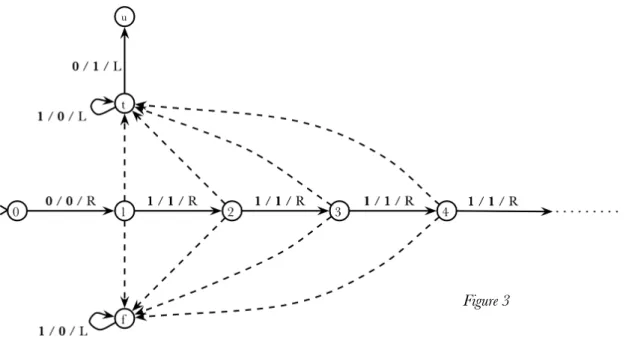
Figure 3 shows how an infinite state Turing machine can compute any function from N to {0, 1}. It is essentially an infinite lookup table which determines for all numbers given as input, what the result should be. By changing the dotted arcs, any such function can be specified – if f(n) = 0, then the dotted arc from state n to state f should be used (which will replace the number on the tape with the representation of 0), while if f(n) = 1, then the dotted arc from state n to state t should be used (which
will replace the number on the tape with the representation of 1). Either way, the transition on the arc should be 1 / 0 / L.
As can be seen here, the tape is only used for the input and output. If one wanted to define inputs by beginning in different states and outputs by terminating in different states, then the tape could be dispensed with altogether.
3.8 Accelerated Turing Machines
In the early 20th Century, Bertrand Russell [42], Ralph Blake [1] and Hermann Weyl [57]
independently proposed the idea of a process that performs its first step in one unit of time and each subsequent step in half the time of the step before. Since 1 + 1/2 + 1/4 + 1/8 + … < 2, such a process
could complete an infinity of steps in two time units. The application of this temporal patterning to Turing machines has been discussed briefly by Ian Stewart [48] and in much more depth by Copeland [16] under the name of accelerated Turing machines. Since Turing’s account of his machines has no mention of how long it takes them to perform an individual step, this acceleration not in conflict with his mathematical conception of a Turing machine.
Consider an accelerated Turing machine, A, that was programmed to simulate an arbitrary Turing machine on arbitrary input. If the Turing machine halts on its input, A then changes the value of a specified square on its tape (say the first square) from a 0 to a 1. If the Turing machine does not halt, then A leaves the special square as 0. Either way, after 2 time units, the first square on A’s tape holds the value of the halting function for this Turing machine and its input.
So far, there has been no difference between an accelerated Turing machine and a standard Turing machine other than the speed at which it operates. In particular, A has not solved the halting problem because Turing Machines are defined to output the value on their tape after they halt. In this case, A
does not halt if its simulated machine does not halt. However, the situation described above suggests a simple change which will allow A to solve the halting problem – we consider the machine’s output to be whatever is on the first square after two time units.
This model of an accelerated Turing machine only computes functions from N to {0,1}, but can be extended to functions from N to N, by designating the odd squares to be used for the special output, with each of them beginning as 0 and only being changed at most once. In this way, a natural number could be output in a unary representation on the special squares. This could even be extended to allowing real output, where all digits of the real would be written in binary on the special squares after two time units of activity.
3.9 Infinite Time Turing Machines
This process of using an infinite computation length can be further extended. In their paper ‘Infinite Time Turing Machines’ [29], Joel Hamkins and Andy Lewis present a model of a Turing machine that operates for transfinite numbers of steps. We could imagine, for instance, a machine that included
an accelerated Turing machine (M) as a part. It could initiate M’s computation, then after two time units, stop M’s movements and reset M to its initial state, leaving the tape as it was at the end of the computation. It could then restart M with its tape head on the first tape square, running it for another two time units. In such a manner, this machine would perform two infinite sequences of steps in succession. One could even imagine a succession of infinitely many restarts, with M performing the whole sequence twice as fast each time, leading to an infinite sequence of infinite sequences of steps. Perhaps surprisingly, such conceptions of infinite sequences followed by further steps are well founded. The number of steps can be seen as the ordinal numbers:
0, 1, 2, 3, ... w, w+1, w+2, ... w⋅2, w⋅2+1, w⋅2+2, ... w2, w2+1, w2+2, ... ww, ...
Here the symbol w represents the first transfinite ordinal. It is also a limitordinal, having no immediate predecessor. After an accelerated Turing machine computes for two time units, it has performed w steps of computation and if the tape is reused on another computation it has performed w⋅2 steps. The infinite sequence of infinite sequences of steps is denoted by w2.
The infinite time Turing machine is a natural extension of the Turing machine to transfinite ordinal times. To determine the configuration of the machine at any successor ordinal time, the new configuration is defined from the old one according to the standard Turing machine rules. At a limit ordinal time, however, the machine's configuration is defined based on all the preceding configurations. The machine goes into a special limit-state and each tape square takes a value as follows:
square n at time a =
†
0, if the square has settled down to 0 1, if the square has settled down to 1 1, if the square alternates between 0 and 1 unboundedly often
Ï Ì Ô Ó Ô
The tape head is placed back on the first square and the machine then continues its computation from this limit-state as it would from any other. As usual, if there is no appropriate step to execute at some point, the machine halts. It can thus perform a finite amount of steps and halt, or an infinite amount of steps and halt, or keep operating through all of the ordinal times and never halt.
Such a machine could compute any recursively enumerable function in w steps, by setting the first square on its tape to 0, then evaluating the function, setting the first square to 1 if f(n) = 1. If f(n) = 1, then after w steps, the first square will hold the value of 1 and if f(n) = 0, then after w steps, the first square will hold the value 0. A similar method also computes any of the recursively enumerable reals.
Since infinite time Turing machines can use the entirety of their tapes during their execution, it is natural to define them to accept infinite input (inscribed on, say, the odd squares) and produce infinite output. This allows them a much greater scope in the functions they can compute, but I shall restrict my study here to those infinite time Turing machines that take only finite input, to allow more direct comparison with the other models discussed.