An efficient reconciliation algorithm for social networks
Nitish Korula
Google Inc. 76 Ninth Ave, 4th Floor
New York, NY
[email protected]
Silvio Lattanzi
Google Inc. 76 Ninth Ave, 4th FloorNew York, NY
[email protected]
ABSTRACT
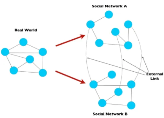
People today typically use multiple online social networks (Facebook, Twitter, Google+, LinkedIn, etc.). Each online network represents a subset of their “real” ego-networks. An interesting and challenging problem is to reconcile these on-line networks, that is, to identify all the accounts belonging to the same individual. Besides providing a richer under-standing of social dynamics, the problem has a number of practical applications. At first sight, this problem appears algorithmically challenging. Fortunately, a small fraction of individuals explicitly link their accounts across multiple networks; our work leverages these connections to identify a very large fraction of the network.
Our main contributions are to mathematically formalize the problem for the first time, and to design a simple, lo-cal, and efficient parallel algorithm to solve it. We are able to prove strong theoretical guarantees on the algorithm’s performance on well-established network models (Random Graphs, Preferential Attachment). We also experimentally confirm the effectiveness of the algorithm on synthetic and real social network data sets.
1.
INTRODUCTION
The advent of online social networks has generated a re-naissance in the study of social behaviors and in the un-derstanding of the topology of social interactions. For the first time, it has become possible to analyze networks and social phenomena on a world-wide scale and to design large-scale experiments on them. This new evolution in social science has been the center of much attention, but has also attracted a lot of critiques; in particular, a longstanding problem in the study of online social networks is to under-stand the similarity between them and “real” underlying social networks [29].
This question is particularly challenging because online social networks are often just a realization of a subset of real social networks. For example, Facebook “friends” are a good representation of the personal acquaintances of a
This work is licensed under the Creative Commons Attribution-NonCommercial-NoDerivs 3.0 Unported License. To view a copy of this li-cense, visit http://creativecommons.org/licenses/by-nc-nd/3.0/. Obtain per-mission prior to any use beyond those covered by the license. Contact copyright holder by emailing [email protected]. Articles from this volume were invited to present their results at the 40th International Conference on Very Large Data Bases, September 1st - 5th 2014, Hangzhou, China.
Proceedings of the VLDB Endowment,Vol. 7, No. 5 Copyright 2014 VLDB Endowment 2150-8097/14/01.
user, but probably a poor representation of her working contacts, while LinkedIn is a good representation of work contacts but not a very good representation of personal re-lationships. Therefore, analyzing social behaviors in any of these networks has the drawback that the results would only be partial. Furthermore, even if certain behavior can be ob-served in several networks, there are still serious problems because there is no systematic way to combine the behavior of a specific user across different social networks and be-cause some social relationships will not appear in any social network. For these reasons, identifying all the accounts be-longing to the same individual across different social services is a fundamental step in the study of social science.
Interestingly, the problem has also very important prac-tical implications. First, having a deeper understanding of the characteristics of a user across different networks helps to construct a better portrait of her, which can be used to serve personalized content or advertisements. In addition, having information about connections of a user across mul-tiple networks would make it easier to construct tools such as “friend suggestion” or “people you may want to follow”. The problem of identifying users across online social net-works (also referred to as the social network reconciliation problem) has been studied extensively using machine learn-ing techniques; several heuristics have been proposed to tackle it. However, to the best of our knowledge, it has not yet been studied formally and no rigorous results have been proved for it. One of the contributions of our work is to give a formal definition of the problem, which is a precur-sor to mathematical analysis. Such a definition requires two key components: A model of the “true” underlying social network, and a model for how each online social network is formed as a subset of this network. We discuss details of our models in Section 3.
Another possible reason for the lack of mathematical anal-ysis is that natural definitions of the problem are demotivat-ingly similar to the graph isomorphism problem.1 In addi-tion, at first sight the social network reconciliation problem seems even harder because we are not looking just for iso-morphism but for similar structures, as distinct social net-works are not identical. Fortunately, when reconciling
so-1In graph theory, an isomorphism between two graphs G
andHis a bijection,f(∗), between the vertex sets ofGand H such that any two verticesuandvofGare adjacent inG if and only if f(u) andf(v) are adjacent inH. The graph isomorphism problem is: Given two graphsG andG0 find an isomorphism between them or determine that there is no isomorphism. The graph isomorphism problem is considered very hard, and no polynomial algorithms are known for it.
cial networks, we have two advantages over general graph isomorphism: First, real social networks are not the adver-sarially designed graphs which are hard instances of graph isomorphism, and second, a small fraction of social network users explicitly link their accounts across multiple networks. The main goal of this paper is to design an algorithm with
provable guaranteesthat is simple, parallelizable and robust to malicious users. For real applications, this last prop-erty is fundamental, and often underestimated by machine learning models.2 In fact, the threat of malicious users is so prominent that large social networks (Twitter, Google+, Facebook) have introduced the notion of ‘verification’ for celebrities.
Our first contribution is to give a formal model for the graph reconciliation problem that captures the hardness of the problem and the notion of an initial set of trusted links identifying users across different networks. Intuitively, our model postulates the existence of a true underlying graph, then randomly generates 2 realizations of it which are per-turbations of the initial graph, and a set of trusted links for some users. Given this model, our next significant contri-bution is to design a simple, parallelizable algorithm (based on similar intuition to the algorithm in [23]) and to prove formally that our algorithm solves the graph reconciliation problem if the underlying graph is generated by well estab-lished network models. It is important to note that our al-gorithm relies on graph structure and the initial set of links of users across different networks in such a way that in order to circumvent it, an attacker must be able to have a lot of friends in common with the user under attack. Thus it is more resilient to attack than much of the previous work on this topic. Finally, we note that any mathematical model is, by necessity, a simplification of reality, and hence it is important to empirically validate the effectiveness of our ap-proach when the assumptions of our models are not satisfied. In Section 5, we measure the performance of our algorithm on several synthetic and “real” data sets.
We also remark that for various applications, it may be possible to improve on the performance of our algorithm by adding heuristics based on domain-specific knowledge. For example, we later discuss identifying common Wikipedia articles across languages; in this setting, machine transla-tion of article titles can provide an additransla-tional useful signal. However, an important message of this paper is that a sim-ple, efficient and scalable algorithm that does not take any domain-specific information into account can achieve excel-lent results for mathematically sound reasons.
2.
RELATED WORK
The problem of identifying Internet users was introduced to identify users across different chat groups or web ses-sions in [24, 27]. Both papers are based on similar intuition, using writing style (stylography features) and a few seman-tic features to identify users. The social network reconcil-iation problem was introduced more recently by Zafarani and Liu in [33]. The main intuition behind their paper is that users tend to use similar usernames across multi-ple social networks, and even when different, search engines
2Approaches based largely on features of a user (such as
her profile) and her neighbors can easily be tricked by a malicious user, who can create a profile locally identical to the attacked user.
find the corresponding names. To improve on these first naive approaches, several machine learning models were de-veloped [3, 17, 20, 25, 28], all of which collect several features of the users (name, location, image, connections topology), based on which they try to identify users across networks. These techniques may be very fragile with respect to ma-licious users, as it is not hard to create a fake profile with similar characteristics. Furthermore, they get lower preci-sion experimentally than our algorithm achieves. However, we note that these techniques can be combined with ours, both to validate / increase the number of initial trusted links, and to further improve the performance of our algo-rithm.
A different approach was studied in [22], where the au-thors infer missing attributes of a user in an online social network from the attribute information provided by other users in the network. To achieve their results, they retrieve communities, identify the main attribute of a community and then spread this attribute to all the user in the commu-nity. Though it is interesting, this approach suffers from the same limitations of the learning techniques discussed above. Recently, Henderson et al. [14] studied which are the most important features to identify a node in a social network, focusing only on graph structure information. They ana-lyzed several features of each ego-network, and also added the notion of recursive features on nodes at distance larger than 1 from a specific node. It is interesting to notice that their recursive features are more resilient to attack by ma-licious users, although they can be easily circumvented by the attacker typically assumed in the social network security literature [32], who can create arbitrarily many nodes.
The problem of reconciling social networks is closely con-nected to the problem of de-anonymizing social networks. Backstrom et al. introduced the problem of deanonymiz-ing social networks in [4]. In their paper, they present 2 main techniques: An active attack (nodes are added to the network before the network is anonymized), and a second passive one. Our setting is similar to that described in their passive attack. In this setting the authors are able to de-sign a heuristic with good experimental results; though their technique is very interesting, it is somewhat elaborate and does not have a provable guarantee.
In the context of de-anonymizing social networks, the work of Narayanan and Shmatikov [23] is closely related. Their algorithm is similar in spirit to ours; they look at the number of common neighbors and other statistics, and then they keep all the links above a specific threshold. There are two main differences between our work and theirs. First, we formulate the problem and the algorithm mathematically and we are able to prove theoretical guarantees for our algo-rithm. Second, to improve the precision of their algorithm in [23] the authors construct a scoring function that is expan-sive to compute. In fact the complexity of their algorithm isO((E1+E2)∆1∆2), whereE1 andE2 are the number of
edges in the two graphs and ∆1and ∆2are the maximum
de-gree in the 2 graphs. Thus their algorithm would be too slow to run on Twitter and Facebook, for example; Twitter has more than 200M users, several of whom have degree more than 20M and Facebook more than 1B users with several users of degree 5K. Instead, in our work we are able to show that a very simple technique based on degree bucketing com-bined with the number of common neighbors suffices to guar-antee strong theoretical guarguar-antees and good experimental
results. In this way we designed an algorithm with sequen-tial complexityO((E1+E2)min(∆1,∆2) log(max(∆1,∆2)))
that can be run inO(log(max(∆1,∆2))) MapReduce rounds.
In this context, our paper can be seen as the first really scalable algorithm for network de-anonymization with the-oretical guarantees. Further, we also obtain considerably higher precision experimentally, though a perfect compari-son across different datasets is not possible. The different contexts also are important: In de-anonymization, the pre-cision of 72% they report corresponds to a significant viola-tion of user privacy. In contrast, we focus on the benefits to users of linking accounts; in a user-facing application, sug-gesting an account with a 28% chance of error is unlikely to be acceptable.
Finally, independently from our work, Yartseva and Gross-glauser [31] recently studied a very similar model focus-ing only on networks generated by the Erd˝os-R´enyi random graph model.
3.
MODEL AND ALGORITHM
In this section, we first describe our formal model and its parameters. We then describe our algorithm and discuss the intuition behind it.
3.1
Model
Recall that a formal definition of the user identification problem requires first a model for the “true” underlying so-cial network G(V, E) that captures relationships between people. However, we cannot directly observe this network; instead, we consider two imperfect realizations or copies G1(V, E1) andG2(V, E2) withE1, E2⊆E. Second, we need
a model for how edges ofE are selected for the two copies E1andE2. This model must capture the fact that users do
not necessarily replicate their entire personal networks on any social networking service, but only a subset.
Any such mathematical models are necessarily imperfect descriptions of reality, and as models become more ‘realis-tic’, they become more mathematically intractable. In this paper, we consider certain well-studied models, and provide complete proofs. It is possible to generalize our mathemat-ical techniques to some variants of these models; for in-stance, with small probability, the two copies could have new “noise” edges not present in the original networkG(V, E), orvertices could be deleted in the copies. We do not fully analyze these as the generalizations require tedious calcula-tions without adding new insights. Our experimental results of Section 5 show that the algorithm performs well even in real networks where the formal mathematical assumptions are not satisfied.
For the underlying social network, our main focus is on thepreferential attachment model [5], which is historically the most cited model for social networks. Though the model does not capture some features of real social networks, the key properties we use for our analysis are those common to online social networks such as a skewed degree distribu-tion, and the fact that nodes have distinct neighbors includ-ing some long-range / random connections not shared with those immediately around them[13, 15]. In the experimental section we will consider also different models and also real social networks as our underline real networks.
For the two imperfect copies of the underlying network we assume thatG1 (respectivelyG2) is created by selecting
each edgee∈Eof the original graphG(V, E) independently
with a fixed probabilitys1 (resp. s2) (See Figure 1.) In the
real world, edges/relationships are not selected truly inde-pendently, but this serves as a reasonable approximation for observed networks. In fact, a similar model has been previ-ously considered by [26], which also produced experimental evidence from an email network to support the independent random selection of edges. Another plausible mechanism for edge creation in social network is thecascade model, in which nodes are more likely to join a new network if more of their friends have joined it. Experimentally, we show that our algorithm performs even better in the cascade model than in the independent edge deletion model.
These two models are theoretically interesting and prac-tically interesting [26]. Nevertheless, in some cases the an-alyzed social networks may differ in their scopes and so the group of friends that a user has in a social network can greatly differ from the group of friends that same user has in the other network. To capture this scenario in the ex-perimental section, we also consider the Affiliation Network model [19] (in which users participate in a number of com-munities) as the underlying social network. For each of G1, G2, and for each community, we keep or delete all the
edges inside the community with constant probability. This highly correlated edge deletion process captures the fact that a user’s personal friends might be connected to her on one network, while her work colleagues are connected on the second network. We defer the detailed description of this experiment to Section 5.
Recall that the user identification problem, givenonlythe graph information, is intractable in general graphs. Even the special case where s1 = s2 = 1 (that is, no edges
have been deleted) is equivalent to the well-studied Graph Isomorphism problem, for which no polynomial-time algo-rithm is known. Fortunately, in reality, there are additional sources of information which allow one to identify a subset of nodes across the two networks: For example, people can use the same email address to sign up on multiple websites. Users often explicitly connect their network accounts, for instance by posting a link to their Facebook profile page on Google+ or Twitter and vice versa. To model this, we assume that there is a set of users/nodes explicitly linked across the two networks G1, G2. More formally, there is a
linking probabilityl(typically,lis a small constant) and each node inV is linked across the networks independently with probability l. (In real networks, nodes may be linked with differing probabilities, but high-degree nodes / celebrities may be more likely to connect their accounts and engage in cross-network promotions; this would be more likely to help our algorithm, since low-degree nodes are less valuable as seeds because they help identify only a small number of neighbors. In the experiments of [23], the authors explic-itly consider high-degree nodes as seeds in the real-world experiments.)
In Section 3.2 below, we present a natural algorithm to solve the user identification problem with a set of linked nodes, and discuss some of its properties. Then, in Section 4, we prove that this algorithm performs well on several well-established network models. In Section 5, we show that the algorithm also works very well in practice, by examining its performance on real-world networks.
3.2
The Algorithm
distributed algorithm that uses only structural information about the graphs to expand the initial set of links into a mapping/identification of a large fraction of the nodes in the two networks.
Before describing the algorithm, we introduce a useful def-inition.
Definition 1. A pair of nodes(u1, u2)withu1∈G1, u2∈
G2 is said to be asimilarity witnessfor a pair(v1, v2)with
v1 ∈ G1, v2 ∈ G2 if u1 ∈ N1(v1), u2 ∈ N2(v2) andu1 has
been linked to / identified withu2.
Here,N1(v1) denotes the neighborhood ofv1 inG1, and
similarlyN2(v2) denotes the neighborhood ofv2 inG2.
Roughly speaking, in each phase of the algorithm, every pair of nodes (one from each network) computes an similar-ity score that is equal to the number of similarsimilar-ity witnesses they have. We then create a link between two nodesv1and
v2 ifv2 is the node inG2 with maximum similarity score to
v1 and vice versa. We then use the newly generated set of
links as input to the next phase of the algorithm.
A possible risk of this algorithm is that in early phases, when few nodes in the network have been linked, low-degree nodes could be mis-matched. To avoid this (improving preci-sion), in theith phase, we only allow nodes of degree roughly D/2i and above to be matched, whereDis a parameter re-lated to the largest node degree. Thus, in the first phase, we match only the nodes of very high degree, and in subsequent phases, we gradually decrease the degree threshold required for matching. In the experimental section we will show in fact that this simple step is very effective, reducing the error rate by more than 33%. We summarize the algorithm, that we called User-Matching, as follows:
Input:
G1(V, E1), G2(V, E2), La set of initial identification links
across the networks,D the maximum degree in the graph a minimum matching scoreT and a specified number of iterationk.
Output:
A larger set of identification links across the networks.
Algorithm:
Fori= 1, . . . , k Forj= logD, . . . ,1
For all the pairs (u, v) withu∈G1 andv∈G2
and such thatdG1(u)≥2
j
anddG2(v)≥2
j
Assign to (u, v) a score equal to the number of similarity witnesses betweenuandv If (u, v) is the pair with highest score in which eitheruorvappear and the score is aboveT add (u, v) toL.
OutputL
WheredGi(u) is the degree of nodeu inGi. Note that the internal for loop can be implemented efficiently with 4 consecutive rounds of MapReduce, so the total running time would consist ofO(klogD) MapReductions. In the exper-iments, we note that even for a small constantk (1 or 2), the algorithm returns very interesting results. The optimal choice of thresholdTdepends on the desired precision/recall tradeoff; higher choices of T improve precision, but in our experiments, we note thatT = 2 or 3 is sufficient for very high precision.
Figure 1: From the real underlying social network, the model generates two random realizations of it, A and B, and some identification links for a subset of the users across the two realizations
4.
THEORETICAL RESULTS
In this section we formally analyze the performance of our algorithm on two network models. In particular, we explain why our simple algorithm should be effective on real social networks. The core idea of the proofs and the algorithm is to leverage high degree nodes to discover all the possible map-ping between users. In fact, as we show here theoretically and later experimentally, high degree nodes are easy to de-tect. Once we are able to detect the high degree nodes, most low degree nodes can be identified using this information.
We start with the Erd˝os-R´enyi (Random) Graph model [11] to warm up with the proofs, and to explore the intuition be-hind the algorithm. Then we move to our main theoretical results, for the Preferential Attachment Model. For simplic-ity of exposition, we assume throughout this section that s1=s2=s; this does not change the proofs in any material
detail.
4.1
Warm up: Random Graphs
In this section, we prove that if the underlying ‘true’ net-work is a random graph generated from the Erd˝os-R´enyi model (also known as G(n, p)), our algorithm identifies al-most all nodes in the network with high probability.
Formally, in theG(n, p) model, we start with an empty graph onnnodes, and insert each of the n2
possible edges independently with probabilityp. We assume thatp <1/6; in fact, any constant probability results in graphs which are much denser than any social network.3 Let G be a graph generated by this process; given this underlying network G, we now construct two partial realizationsG1, G2 as
de-scribed by our model of Section 3.
We note that the probability a specific edge exists inG1or
G2 isps. Also, ifnpsis less than (1−ε) lognforε >0, the
graphsG1andG2 are not connected w.h.p. [11]. Therefore,
we assume thatnps > clognfor some constantc.
In the following we identify the nodes inG1withu1, . . . , un
and the nodes inG2 withv1, . . . , vn, where nodesui andvi
correspond to the same nodeiinG. In the first phase, the expected number of similarity witnesses for a pair (ui, vi) is 3In fact, the proof works even withp= 1/2, but it requires
more care. However, when p is too close to 1, G is close to a clique and all nodes have near-identical neighborhoods, making it impossible to distinguish between them.
(n−1)ps2·l. This follows because the expected number of
neighbors ofiinGis (n−1)p, the probability that the edge to a given neighbor survives in bothG1 andG2 iss2, and
the probability that it is initially linked isl. On the other hand, the expected number of similarity witnesses for a pair (ui, vj), withi6=jis (n−2)p2s2·l; the additional factor of
pis because a given other node must have an edge to both iand j, which occurs with probabilityp2. Thus, there is a
factor ofpdifference between the expected number of sim-ilarity witnesses a nodeui has with its true matchvi and
with some other nodevj, withi6=j. The main intuition is
that this factor ofp <1 is enough to ensure the correctness of algorithm. We prove this by separately considering two cases: Ifpis sufficiently large, the expected number of sim-ilarity witnesses is large, and we can apply a concentration bound. On the other hand, ifp is small,np2s2 is so small that the expected number of similarity witnesses is almost negligible.
We start by proving that in the first case there is always a gap between a real and a false match.
Theorem 1. If(n−2)ps2l≥24 logn(that is,p >s242l
logn n−2),
w.h.p. the number of first-phase similarity witnesses between
uiandviis at least(n−1)ps2l/2. The number of first-phase
similarity witnesses betweenui andvj, withi6=jis w.h.p.
at most(n−2)ps2l/2.
Proof. We prove both parts of the lemma using Chernoff Bounds (see, for instance, [10]).
Let consider a pair for node j. Let Yi be a r.v. such
that Yi = 1 if nodeui ∈ N1(uj) andvi ∈ N2(vj), and if
(ui, vi) ∈ L, where L is the initial seed of links acrossG1
andG2. Then, we haveP r[Y1= 1] =ps2l. IfY =Pn
−1 i=1 Yi,
the Chernoff bound implies that P r[Y < (1−δ)E[Y]] ≤
e−E[Y]δ2/2. That is, P r
Y <1
2(n−1)ps
2
l
≤e−E[Y]/8< e−3 logn= 1/n3 Now, taking the union bound over thennodes inG, w.h.p. every node has the desired number of first-phase similarity witnesses with its copy.
To prove the second part, suppose w.l.o.g. that we are considering the number of first-phase similarity witnesses betweenui and vj, with i =6 j. Let Yi = 1 if node uz ∈
N1(ui) and vz ∈ N2(vj), and if (uz, vx) ∈ L. If Y = Pn−2
i=1 Yi, the Chernoff bound implies that P r[Y > (1 +
δ)E[Y]]≤e−E[Y]δ2/4. That is,
P r
Y > 1
2p(n−2)p
2
s2l= (n−2)ps
2
l 2
≤e−E[Y](21p−1)
2/4
=e−2p(21p−1)
23 logn
≤1/n3
where the last inequality comes from the fact thatp <1/6. Taking the union bound over alln(n−1) unordered pairs of nodesui, vjgives the fact that w.h.p., every pair of different
nodes does not have too many similarity witnesses. The theorem above implies that when p is sufficiently large, there is a gap between the number of similarity wit-nesses of pairs of nodes that correspond to the same node and a pair of nodes that do not correspond to the same node. Thus the first-phase similarity witnesses are enough to com-pletely distinguish between the correct copy of a node and possible incorrect matches.
It remains only to consider the case when p is smaller than the bound required for Theorem 1. This requires the following useful lemma.
Lemma 2. LetB be a Bernoulli random variable, which is 1 with probability at most x, and 0 otherwise. Ink in-dependent trials, let Bi denote the outcome of the ithtrial,
and letB(k) =Pk
i=1Bi: If kx iso(1), the probability that
B(k) is greater than2is at mostk3x3/6 +o(k3x3).
Proof. The probability thatB(k) is at most 2 is given by: (1−x)k+kx·(1−x)k−1+ k
2
x2·(1−x)k−2. Using
the Taylor series expansion for (1−x)k−2, this is at most 1−k3x3/6−o(k3x3).
When we run our algorithm on a graph drawn fromG(n, p), we set the minimum matching threshold to be 3.
Lemma 3. Ifp≤s242l logn
n−2, w.h.p., algorithmUser-Matching
never incorrectly matches nodes uiandvj withi6=j.
Proof. Suppose for contradiction the algorithm does in-correctly match two such nodes, and consider the first time this occurs. We use Lemma 2 above. Let Bz denote the
event that the vertexzis a similarity witness foruiandvj.
In order for Bz to have occurred, we must have uz in
N1(Ui) andvz inN2(vj) and (uz, vz)∈L. The probability
that Bz = 1 is therefore at mostp2s2. Note that eachBz
is independent of the others, and that there aren−2 such events. AspisO(logn/n), the conditions of Lemma 2 apply, and hence the probability that more than 2 such events occur is at most (n−2)3p6s6. ButpisO(logn/n), and hence this event occurs with probability at most O(log6n/n3). Tak-ing the union bound over all n(n−1) unordered pairs of nodesui, vjgives the fact that w.h.p., not more than 2
sim-ilarity witnesses can exist for any such pair. But since the minimum matching threshold for our algorithm is 3, the al-gorithm does not incorrectly match this pair, contradicting our original assumption.
Having proved that our algorithm does not make errors, we now show that it identifies most of the graph.
Theorem 4. Our algorithm identifies1−o(1)fraction of the nodes w.h.p.
Proof. Note that the probability that a node is identified is 1−o(1) by the Chernoff bound because in expectation it has Ω(logn) similarity witnesses. So in expectation, we identify 1−o(1) fraction of the nodes. Furthermore, by applying the method of bounded difference [10] (each node affects the final result at most by 1), we get that the result holds also with high probability.
4.2
Preferential Attachment
The preferential attachment model was introduced by Barab´asi and Albert in [5]. In this paper we consider the formal def-inition of the model described in [6].
Definition 2. [PA model]. Let Gmn, m being a fixed
parameter, be defined inductively as follows: • Gm
1 consists of a single vertex withmself-loops.
• Gm
n is built from Gmn−1 by adding a new node u
to-gether with m edges e1u = (u, v1), . . . , emu = (u, vm)
the sum of the degrees of all the nodes when the edgeei u
is added. The endpoint vi is selected with probability deg(vi)
Mi+1, with the exception of nodeu, which is selected
with probability d(u)+1M
i+1.
The PA model is the most celebrated model for social net-works. Unlike the Erd˝os-R´enyi model, in which all nodes have roughly the same degree, PA graphs have a degree distribution that more accurately resembles the skew de-gree distribution seen in real social networks. Though more evolved models of social networks have been recently intro-duced, we focus on the PA model here because it clearly il-lustrates why our algorithm works in practice. Note that the power-law distribution of the model complicates our proofs, as the overwhelming majority of nodes only have constant degree (≤2m), and so we can no longer simply apply con-centration bounds to obtain results that hold w.h.p. For a (small) constant fraction of the nodesu, there does not exist any nodez such thatuz ∈N1(ui) andvz∈N2(vi); we
can-not hope to identify these nodes, as they have no neighbors “in common” on the two networks. In fact, if m= 4 and s= 1/2, roughly 30% of nodes of “true” degreemwill be in this situation. Therefore, to be able to identify a reasonable fraction of the nodes, one needsmto be at least a reason-ably large constant; this is not a serious constraint, as the median friend count on Facebook, for instance, is over 100. In our experimental section, we show that our algorithm is effective even with smallerm.
We now outline our overall approach to identify nodes across two PA graphs. In Lemma 11, we argue that for the nodes of very high degree, their neighborhoods are differ-ent enough that we can apply concdiffer-entration argumdiffer-ents and uniquely identify them. For nodes of intermediate degree (log3n) and less, we argue in Lemma 10 that two distinct nodes of such degree are very unlikely to have more than 8 neighbors in common. Thus, running our algorithm with a minimum matching threshold of 9 guarantees that there are no mistakes. Finally, we prove in Lemma 12 that when we run the algorithm iteratively, the high-degree nodes help us identify many other nodes, these nodes together with the high-degree nodes in turn help us identify more, and so on: Eventually, the probability that any given node is uniden-tified is less than a small constant, which implies that we correctly identify a large fraction of the nodes.
Interestingly, we notice in our experiments that on real networks, the algorithm has the same behavior as on PA graphs. In fact, as we will discuss later, the algorithm is al-ways able to identify high-degree/important nodes and then, using this information, identify the rest of the graph.
Technical Results: The first of the three main lemmas we need, Lemma 11, states that we can identify all of the high-degree nodes correctly. To prove this, we need a few techni-cal results. These results say that all nodes of high degree join the network early, and continue to increase their degree significantly throughout the process; this helps us show that high-degree nodes do not share too many neighbors.
4.2.1
High degree nodes are early-birds
Here we will prove formally that the nodes of degree Ω(log2n)
join the network very early; this will be useful to show that two high degree nodes do not share too many neighbors.
Lemma 5. Let Gmn be the preferential attachment graph
obtained after n steps. Then for any node v inserted after
timeψn, for any constantψ >0,dn(v)∈o(log2n)with high
probability, wheredn(v) is the degree of nodesvat timen.
Proof. It is possible to prove that such nodes have ex-pected constant degree, but unfortunately, it is not trivial to get a high probability result from this observation be-cause of the inherent dependencies that are present in the preferential attachment model. For this reason we will not prove the statement directly, but we will take a short de-tour inspired by the proof in [18]. In particular we will first break the interval in a constant number of small intervals. Then we will show that in each interval the degree ofvwill increase by at most O(logn) with high probability. Thus we will be able to conclude that at the end of the process the total degree ofvis at mostO(logn)(recall that we only have a constant number of interval).
As mentioned above we analyze the evolution of the degree of v in the intervalψn to n by splitting this interval in a constant number of segments of lengthλn, for some constant λ >0 to be fixed later. Now we can focus on what happens to the degree ofvin the interval (t,·λn+t] ifdt(v)≤Clogn,
for some constant C≥1 andt≥ψn. Note that if we can prove thatdλn+t≤C0logn, for some constantC0≥0 with
probability 1−o n−2
, we can then finish the proof by the arguments presented in the previous paragraph.
In order to prove this, we will take a small detour to avoid the dependencies in the preferential attachment model. More specifically, we will first show that this is true with high probability for a random variableX for which it is easy to get the concentration result. Then we will prove that the random variableX stochastically dominates the increase in the degree ofv. Thus the result will follow.
Now, let us define X as the number of heads that we get when we toss a coin which gives head with probability
C0logn
t for λn times, for some constant C
0
≥ 13C. It is possible to see that:
E[X] = C 0
logn t λn≤
C0logn ψn λn≤
C0λlogn ψ
Now we fixλ= 100ψ and we use the Chernoff bound to get the following result:
Pr
X >C 0
−C 2 logn
= Pr X >
100(C0−C) 2C0
E[X]
!
≤ 2− C0
100logn
100(C0 −C) 2C0
≤ 2−
(6C0) 13 logn
≤ 2−6 logn∈O n−3
So we know that the value ofX is bounded by C0−2Clogn with probability O n−3
. Now, note that until the degree of v is less than C0logn the probability that v increases its degree in the next step is stochastically dominated by the probability that we get an head when we toss a coin which gives head with probability C0logt n. To conclude our algorithm we study the probability thatvbecome of degree
C0logn
t precisely at timet≤t
∗≤
λn. Note that until timet∗ vhas degree smaller than C0logt n and so it is dominated by the coin. But we already know that when we toss such a coin at mostλntimes the probability of gettingC0−C
2 lognheads
is inO n−3
vreach degreeC0lognat timet∗isO(n−3). Thus by using
the union bound on all the possiblet∗,vwill get to degree C0lognwith probabilityO(n−2).
At this point we can finish the proof by taking the union bound on all the segments(recall that they are constant) (ψn, ψ+λn],(ψ+λn, ψn+ 2λ],· · · and on the number of nodes and we get that all the nodes that join the network after timeψnhave degree that is upper bounded byC00logn for some constantC00≥0 with probabilityO(n−1).
4.2.2
The rich get richer
In this section we study another fundamental property of the preferential attachment, which is that nodes with degree bigger than log2n continue to increase their degree signifi-cantly throughout the process. More formally:
Lemma 6. Let Gmn be the preferential attachment graph
obtained after n steps. Then with high probability for any nodevof degreed≥log2nand for any fixed constant≥0, a 1
3 fraction of the neighbors ofvjoined the graph after time
n.
Proof. By Lemma 5 above, we know thatvjoined the network before timenfor any fixed constant≥0. Now we consider two cases. In the first,dn(v)≤ 12log2n, in which
case the statement is true because the final degree is bigger than log2n. Otherwise, we have thatdn(v)> 12log2n, in
this case the probability thatvincrease its degree at every time step afterndominates the probability that a toss of a biased coin which gives head with probability log2mn2n comes up head. Now consider the random variableX that counts the number of heads when we toss a coin that lands head with probability log2mn2n for (1−)mntimes. The expected value ofX is:
E[X] = log
2n
2mn(1−)mn= 1−
2 log
2
n Thus using the Chernoff bound:
Pr
X≤ 1−2
2 log
2
n
≤ exp
−1
2
1−
1−
log2n
∈ O(n−2)
Thus with probabilityO(1−n−2)Xis bigger that1−22log2n but as mentioned before the increase in the degree of v stochastically dominatesX. Thus taking the union bound on all the possiblevwe get that the statement holds with probability equal toO(1−n−1). Thus the claim follows.
4.2.3
First-mover advantage
Lemma 7. Let Gmn be the preferential attachment graph
obtained after n steps. Then with high probability all the nodes that join the network before timen0.3 have degree at leastlog3n.
Proof. To prove this theorem we will use some results from [9], but before we need to introduce another model equivalent to the preferential attachment. In this new pro-cess instead of constructingGm
n, we first constructG1nmand
then we collapse the vertices 1,· · ·, mto construct the first vertex, the vertex between m+ 1,· · ·2m to construct the second vertex and so on so for. It is not hard to see that this new model is equivalent to the preferential attachment. Now we can prove our technical theorem.
Now we can state two useful equation from the proof of Lemma 6 in [9]. Consider the model Gnm1 . Let Dk =
dnm(v1) +dnm(v2) +· · ·+dnm(vk), where dnm(vi) is the
degree of a node inserted at timeiat timenm. Thenk≥1 we have:
Pr
|Dk−2
√
kmn| ≥3pmnlog(mn)
≤(mn)−2 (1) From the same paper we also have that if 0≤d≤mn−k−s, we can derive from equation (23) that
Pr(dn(vk+1) =d+ 1|Dk−2k=s)≤
s+d
2N−2k−s−d (2) From 1 we can derive that:
Pr
Dk−2k≥3 p
mnlog(mn) + 2√kmn−2k
≤(mn)−2
PrDk−2k≥5 p
kmnlog(mn)≤(mn)−2 Thus we get that:
Pr(dn(vk+1)<log3n) = log3n−1
X
0
Pr(dn(vk+1) =i)
≤ PrDk−2k≥3 p
mnlog(mn) + 2√kmn−2k
+
log3n−1 X
i=0
5√kmnlog(mn) X
j=0
Pr (Dk−2k=j)
Pr(dn(vk+1) =i|Dk−2k=j)
≤ (mn)−2+
log3n−1 X
i=0
Prdn(vk+1) =i|Dk−2k
= 5pmnlog(mn)
≤ (mn)−2+
log3n−1 X
i=0
5p
mnlog(mn) +i−1 2mn−2k−5pmnlog(mn)−i+ 1
∈ O
log4(n)
√
n
where we assumed thatk∈O
n13
.
So now by union bounding on the first mn0.3 nodes we
obtain that with high probability inGnm1 all the nodes have
degree bigger than log2n. But this implies in turn the state-ment of the theorem by construction ofGnm
1 .
Now we state our last technical lemma on handling prod-uct of generalized harmonic, the proof of this lemma is de-ferred to the final version of the paper:
Lemma 8. Letaandbbe constant greater than0. Then:
nb−2 X
i=na
nb−1 X
j>i nb X
z>j
1 i2j2z2 ∈O
1 n3a
Completing the Proof: We now use the technical lemmas above to complete our proof for the preferential attachment model.
Lemma 9. For a node u with degree d, the probability that it is incident to a node arriving at time i is at most
Proof. If nodei arrives after u, the probability that i is adjacent touis at most the given value, since there are m(i−1) edges existing in the graph already, and we take the union bound over themedges incident toi. Ifiarrivesbefore
u, lettdenote the time at whichuarrives. From Lemma 6 of [9], the degree ofiat t is at most√tilog3nw.h.p.. But there are (t−1)medges already in the graph at this time, and since uhasmedges incident to it, the probability that one of them is incident toiis at most log3n
√
t
√
i(t−1) ≤log 3
n/(i−1). Lemma 10. W.h.p, for any pair of nodes u, v of degree <log3n,|N(u)∩N(v)| ≤8.
Proof. From Lemma 7, nodesuandvmust have arrived after timet=n0.3. Let a, bbe constants such that 0.3 < a < b <1 andb≤3/2a−ε for some constant ε >0. We first show that the probability that any two nodesu, vwith degree less than log3n and arriving before timenb have 3
or more common neighbors between na and nb is at most n−ε. This implies that, setting a to 0.3, nodes u and v have at most 2 neighbors betweenna andn3a/2−ε, at most
2 betweenn3a/2−εand n9a/4, and at most 2 between n9a/4 andn27a/8 > n, for a total of 6 overall. Similarly, we show thatuandvhave at most 2 neighbors arriving beforen0.3,
which completes the lemma.
From Lemma 9 above, the probability that a node arriving at timeiis incident touandvis at most (log3n/(i−1))2.
(The events are not independent, but they are negatively correlated.) The probability that 3 nodesi, j, kare all inci-dent to bothuandv, then, is at most (log3n)6/((i−1)(j−
1)(k−1))2. Therefore, for a fixedu, v, the probability that
some 3 nodes are adjacent touandvis at most:
log18n
nb
X
i=na
nb
X
j=na
nb
X
k=na
1
((i−1)(j−1)(k−1))2
≤ log18n
1 na −
1 nb
3
There are at most nb choices for each ofuandv; taking the union bound, the probability that any pairu,vhave 3 or more neighbors in common is at most n2b−3alog18n = n−2εlog18n.
So, by setting the matching threshold to 9, the algorithm never makes errors; we now prove that it actually detects a lot of good new links.
Lemma 11. The algorithm successfully identifies any node of degree≥4 log2n/(s2l).
Proof. For any nodev of degree d(v) ≥4 log2n/(s2l), the expected number of similarity witnesses it has with its copy during the first phase is d(v)s2l; using the Chernoff
Bound, the probability that the number is less than 7/8 of its expectation is at most exp(−d(v)s2l/128)≤exp(−log2n/32) =
1
nlogn/32. Therefore, with very high probability, every node
vof degreed(v) has at least 7/8·d(v)s2lfirst-phase similarity
witnesses with its copy.
On the other hand, how many similarity witnesses can nodevhave with a copy of a different nodeu? Fixε >0, and first consider potential similarity witnesses that arrive before timet=εn; later, we consider those that arrive af-ter this time. From Lemma 6, we have dt(v) ≤ (2/3 +
ε)d(v). Even if all of these neighbors of v are also inci-dent to u, the expected number of similarity witnesses for (u, v) is at mostdt(v)s2l. Now consider the neighbors ofv
that arrive after time εn. Each of these nodes is a neigh-bor of u with probability ≤ d(u)/(2mεn). But d(u) ≤
˜
O(√n), and hence each of the neighbors ofvis a neighbor ofuwith probabilityo(1/n1/2−δ). Therefore, the expected number of similarity witnesses for (u, v) among these nodes is at most d(v)s2l/n1/2−δ. Therefore, the total expected number of similarity witnesses is at most (2/3 +ε)d(v)s2l.
Again using the Chernoff Bound, the probability that this is at least 7/8·d(v)s2lis at most exp(−3/4d(v)s2l·/64) = exp(−3 log2n/64), which is at most 1
n3 logn/64.
To conclude, we showed that with very high probability, a high-degree nodevhas at least 7/8·d(v)s2lfirst-phase sim-ilarity witnesses with its copy, and has fewer than this num-ber of witnesses to the copy of any other node. Therefore, our algorithm correctly identifies all high-degree nodes.
From the two preceding lemmas, we identify all the high-degree nodes, and make no mistakes on the low-high-degree nodes. It therefore remains only to show that we have a good suc-cess probability for the low-degree nodes. In the lemma below, we show this whenms2≥22. We note that one still obtains good results even with a higher or lower value of ms2, but it appears difficult to obtain a simple closed-form
expression for the fraction of identified nodes. For ease of exposition, we present the case of ms2 ≥22 here, but the proof generalizes in the obvious way.
Lemma 12. Suppose ms2 ≥ 22. Then, w.h.p., we
suc-cessfully identify at least 97%of the nodes.
Proof. We have already seen that all high-degree nodes (those arriving before time n0.3) are identified in the first phase of the algorithm. Note also that it never makes a mis-take; it therefore remains only to identify the lower-degree nodes. We describe a sequence of iterations in which we bound the probability of failing to identify other nodes.
Consider a sequence of roughly n0.75 iterations, in each
of which we analyze n0.25 nodes. In particular, iteration i contains all nodes that arrived between timen0.3+ (i−
1)n0.25and timen0.3+i·n0.25. We argue inductively that
after iteration i, w.h.p. the fraction of nodes belonging to this iteration that are not identified is less than 0.03, and the total fraction of degree incident to unidentified nodes is less than 0.08. Since this is true for each i, we obtain the lemma.
The base case of nodes arriving beforen0.3 has already been handled. Now, note that during any iteration, the total degree incident to nodes of this iteration is at most 2mn0.25 n0.3. Thus, when each node of this iteration, the probability that any of itsmedges is incident to another node of this iteration is less than 0.01.
Consider any of them edges incident to a given node of this iteration. For each edge, we say it isgood if it survives in both copies of the graph, and is incident to an identified node from a previous iteration. Thus, the probability that an edge is good is at leasts2·(0.99×0.92). Sincems2>22,
the expected number of good edges is greater than 20. The node will be identified if at least 8 of its edges are good; applying the Chernoff bound, the probability that a given node is unidentified is at most exp(−3.606)<0.02717.
Since this is true for each node of this iteration, regard-less of the outcomes for previous nodes of the iteration, we
can apply concentration inequalities even though the events are not independent. In particular, the number of iden-tified nodes stochastically dominates the number of suc-cesses inn0.25independent Bernoulli trials with probability
1−exp(−3.606) (see, for example, Theorem 1.2.17 of [21]). Again applying the Chernoff Bound, the probability that the fraction of unidentified nodes exceeds 0.03 is at most exp(0.27n0.25∗0.01/4), which is negligible. To complete
the induction, we need to show that the fraction of total degree incident to unidentified nodes is at most 0.08. To observe this, note that the increase in degree is 2mn0.25; the
unidentified fraction increases if the new nodes are uniden-tified (but we have seen the expected contribution here is at most 0.02717mn0.25), or if the “other” endpoint is
an-other node of this iteration (at most 0.01mn0.25), or if the “other” endpoint is an unidentified node (in expectation, at most 0.08mn0.25). Again, a simple concentration argument
completes the proof.
5.
EXPERIMENTS
In this section we analyze the performance of our algo-rithm in different experimental settings. The main goal of this section is to answer the following eight questions:
• Are our theorems robust? Do our results depend on the constants that we use or are they more general?
• How does the algorithm scale on very large graphs?
• Does our algorithm work only for an underlying “real” network generated by a random process such as Pref-erential Attachment, or does it work for real social networks?
• How does the algorithm perform when the two net-works to be matched are not generated by indepen-dently deleting edges, but by a different process like a cascade model?
• How does the algorithm perform when the two net-works to be matched have different scopes? Is the algorithm robust to highly correlated edge deletion?
• Does our model capture reality well? In more realistic scenarios, with distinct but similar graphs, does the algorithm perform acceptably?
• How does our algorithm perform when the network is under attack? Can it still have high precision? Is it easy for an adversary to trick our algorithm?
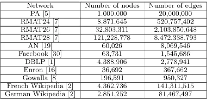
• How important is it to bucket nodes by degree? How big is the impact on the algorithm’s precision? How does our algorithm compare with a simple algorithm that just counts the number of common neighbors? To answer these eight questions, we designed 4 different experiments using 6 different publicly available data sets. These experiments are increasingly challenging for our algo-rithm, which performs well in all cases, showing its robust-ness. Before entering into the details of the experiments, we describe briefly the basic datasets used in the paper. We use synthetic random graphs generated by the Preferential Attachment [5], Affiliation Network [19], and RMAT [7] pro-cesses; we also consider an early snapshot of the Facebook graph [30], a snapshot of DBLP [1], the email network of Enron [16], a snapshot of Gowalla [8] (a social network with location information), and Wikipedia in two languages [2]. In Table 1 we report some general statistics on the networks.
Network Number of nodes Number of edges PA [5] 1,000,000 20,000,000 RMAT24 [7] 8,871,645 520,757,402 RMAT26 [7] 32,803,311 2,103,850,648 RMAT28 [7] 121,228,778 8,472,338,793 AN [19] 60,026 8,069,546 Facebook [30] 63,731 1,545,686 DBLP [1] 4,388,906 2,778,941 Enron [16] 36,692 367,662 Gowalla [8] 196,591 950,327 French Wikipedia [2] 4,362,736 141,311,515 German Wikipedia [2] 2,851,252 81,467,497
Table 1: The original 11 datasets.
Figure 2: The number of corrected pairs detected with different threshold for the preferential attach-ment model with random deletion. The precision is not shown in the plot because it is always 100%.
Robustness of our Theorems: To answer the first ques-tion, we use as an underlying graph the preferential at-tachment graph described above, with 1,000,000 nodes and m= 20. We analyze the performance of our algorithm when we delete edges with probabilitys= 0.5 and with different seed link probabilities. The main goal of this experiment is to show that the values ofm, sneeded in our proof are only required for the calculations; the algorithm is effective even with much lower values. With the specified parameters, for the majority of nodes, the expected number of neighbors in the intersection of both graphs is 5. Nevertheless, as shown in Figure 2, our algorithm performs remarkably well, making zero errors regardless of the seed link probability. Further, it recovers almost the entire graph. Unsurprisingly, lower-ing the threshold for our algorithm increases recall, but it is interesting to note that in this setting, it does not affect precision at all.
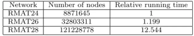
Efficiency of our algorithms: Here we tested our algo-rithms with datasets of increasing size. In particular we generate 3 synthetic random graphs of increasing size using the RMAT random model. Then we use the three graphs as the underlying “real” networks and we generate 6 graphs from them with edges surviving with probability 0.5. Fi-nally we analyze the running time of our algorithm with seed link probability equal to 0.10. As shown in Table 2, using the same amount of resources, the running time of the algorithm increases by at most a factor 12.544 between the smallest and the largest graph.
Robustness to other models of the underlying graph:
Network Number of nodes Relative running time RMAT24 8871645 1
RMAT26 32803311 1.199 RMAT28 121228778 12.544
Table 2: The relative running time of the algorithm on three RMAT graphs as a function of numbers of nodes in the graph.
Pr Threshold 5 Threshold 4 Threshold 2 Good Bad Good Bad Good Bad 20% 23915 0 28527 53 41472 203 10% 23832 49 32105 112 38752 213 5% 11091 43 28602 118 36484 236 Pr Threshold 5 Threshold 4 Threshold 3 Good Bad Good Bad Good Bad 10% 3426 61 3549 90 3666 149
Table 3: Results for Facebook (Top) and Enron (Bottom) under the random deletion model. Pr de-notes the seed link probability.
and consider the snapshots of Facebook and the Enron email networks as our initial underlying networks. For Facebook, edges survive either with probabilitys = 0.5 ors = 0.75, and we analyze performance of our algorithm with different seed link probabilities. For Enron, which is a much sparser network, we delete the edges with probabilitys = 0.5 and analyze performance of our algorithm with seed link proba-bility equal to 0.10. The main goal of these experiments is to show that our algorithm has good performance even out-side the boundary of our theoretical results even when the underlying network is not generated by a random model.
In the first experiment with Facebook, when edges survive with probability 0.75, there are 63584 nodes with degree at least 1 in both networks.4 In the second, with edges
sur-viving with probability 0.5, there are 62854 nodes with this property. In this case, the results are also very strong; see Table 3. Roughly 28% of nodes have extremely low degree (≤5), and so our algorithm cannot obtain recall as high as in the previous setting. However, we identify a very large fraction of the roughly 45250 nodes with degree above 5, and the precision is still remarkably good; in all cases, the error is well under 1%. Table 2 presents the full results for the harder case, with edge survival probability 0.5. With edge survival probability 0.75 (not shown in the table), per-formance is even better: At threshold 2 and the lowest seed link probability of 5%, we correctly identify 46626 nodes and incorrectly identify 20, an error rate of well under 0.05%. In the case of Enron, the original email network is very sparse, with an average degree of approximately 20; this means that each copy has average degree roughly 10, which is much sparser than real social networks. Of the 36,692 original nodes, only 21,624 exist in the intersection of the two copies; over 18,000 of these have degree≤ 5, and the average degree is just over 4. Still, with matching threshold 5, we identify almost all the nodes of degree 5 and above, and even in this very sparse graph, the error rate among newly identified nodes is 4.8%.
4Note that we can only detect nodes which have at least
degree 1 in both networks
Figure 3: The number of corrected pairs detected with different threshold for the two Facebook graphs generated by the Independent Cascade Model. The plot does not show precision, since it is always 100%.
Pr Threshold 4 Threshold 3 Threshold 2 Good Bad Good Bad Good Bad 10% 54770 0 55863 0 55942 0
Table 4: Results for the Affiliation Networks model under correlated edge deletion probability.
Robustness to different deletion models: We now turn our attention to the fourth question: How much do our re-sults depend on the process by which the two copies are generated? To answer this, we analyze a different model where we generate the two copies of the underlying graph using the Independent Cascade Model of [12]. More specif-ically, we construct a graph starting from one seed node in the underlying social network and we add to the graph the neighbors of the node with probability p = 0.05. Subse-quently, every time we add a node, we consider all its neigh-bors and add each of them independently with probability p= 0.05 (note that we can try to add a node to the graph multiple times).
The results in this cascade model are extremely good; in fact, for both Facebook and Enron we have 0 errors; as shown for Facebook in Figure 3, we are able to identify al-most all the nodes in the intersection of the two graphs (even at seed link prob. 5%, we identify 16,273/16533 = 98.4%).
Robustness to correlated edge deletion: We now ana-lyze one of the most challenging scenarios for our algorithm where, independently in the two realizations of the social network, we delete all or none of the edges in a commu-nity. For this purpose, we consider the Affiliation Networks model [19] as the underlying real network. In this model, a bipartite graph of users and interests is constructed using a preferential attachment-like process and then two users are connected in the network if and only if they share an inter-est (for the model details, refer to [19]). To generate the two copies in our experiment, we delete the interests inde-pendently in each copy with probability 0.25, and then we generate the graph using only the surviving interests. Note that in this setting, the same node in the two realizations can have very different neighbors. Still, our algorithm has very high precision and recall, as shown in Table 4.
Real world scenarios: Now we move to the most chal-lenging case, where the two graphs are no longer generated by a mathematical process that makes 2 imperfect copies
of the same underlying network. For this purpose, we con-duct two types of experiments. First, we use the DBLP and the Gowalla datasets in which each edge is annotated with a time, and construct 2 networks by taking edges in disjoint time intervals. Then we consider the French- and German-language Wikipedia link graph.
From the co-authorship graph of DBLP, the first network is generated by considering only the publications written in even years, and the second is generated by considering only the publications written in odd years. Gowalla is a social network where each user could also check-in to a location (each check-in has an associated timestamp). Using this information we generate two Gowalla graphs; in the first graph, we have an edge between nodes if they are friends and if and only if they check-in to approximately the same location in an odd month. In the second, we have an edge be-tween nodes if they are friends and if and only if they check-in check-in approximately the same location check-in an even month.
Note that for both DBLP and Gowalla, the two con-structed graphs have a different set of nodes and edges, with correlations different from the previous independent deletion models. Nevertheless we will see that the intersection is big enough to retrieve a good part of the networks.
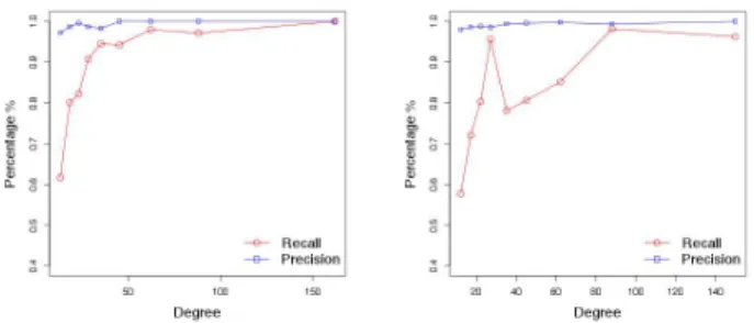
In DBLP, there are 380,129 nodes in the intersection of the two graphs, but the considerable majority of them have extremely low degree. Over 310K have degree less than 5 in the intersection of the two graphs, and so again we cannot hope for extremely high recall. However, we do find consid-erably more nodes than in the input set. We start with a 10% probability of seed links, resulting in 32087 seeds; how-ever, note that most of these have extremely low degree, and hence are not very useful. As shown in table 5, we have nearly 69,000 nodes identified, with an error rate of under 4.17%. Note that we identify over half the nodes of degree at least 11, and a considerably larger fraction of those with higher degree. We include a plot showing precision and re-call for nodes of various degrees (Figure 4).
For Gowalla, there are 38103 nodes in the intersection of the two graphs, of which over 32K have degree≤5. We start with 3800 seeds, of which most are low-degree and hence not useful. We identify over 4000 of the (nearly 6000) nodes of degree above 5, with an error rate of 3.75%. See Table 5 and Figure 4 for more details.
Finally for a still more challenging scenario, we consider a case where the 2 networks do not have any common source, but yet may have some similarity in their structure. In par-ticular, we consider the case of the French- and German-language Wikipedia sites, which have 4.36M and 2.85M nodes respectively. Wikipedia also maintains a set of inter-language links, which connect corresponding articles in a pair of lan-guages; for French and German, there are 531710 links, cor-responding to only 12.19% of the French articles. The rel-atively small number of links illustrates the extent of the difference between the French and German networks. Start-ing with 10% of the inter-language links as seeds, we are able to nearly triple the number of links (including finding a number of new links not in the input inter-language set), with an error rate of 17.5% in new links. However, some of these mistakes are due to human errors in Wikipedia’s inter-language links, while others mistake French articles to closely connected German ones; for instance, we link the French article for Lee Harvey Oswald (the assassin of Pres-ident Kennedy) to the German article on the assassination.
Pr Threshold 5 Threshold 4 Threshold 2 Good Bad Good Bad Good Bad 10 42797 58 53026 641 68641 2985
Pr Threshold 5 Threshold 4 Threshold 2 Good Bad Good Bad Good Bad 10 5520 29 5917 48 7931 155
Pr Threshold 5 Threshold 3 Good Bad Good Bad 10 108343 9441 122740 14373
Table 5: Results for DBLP (Top), Gowala (Middle), and Wikipedia (Bottom)
Figure 4: Precision and Recall vs. Degree Distribution for Gowala (left) and DBLP (right).
Robustness to attack: We now turn our attention to a very challenging question: what is the performance of our algorithm when the network is under attack? In order to an-swer this question, we again consider the Facebook network as the underlying social network, and from it we generate two realizations with edge probability 0.75. Then, in order to simulate an attack, in each network for each node vwe create a malicious copy of it, w, and for each nodeu con-nected to vin the network (that is,u∈N(v)), we add the edge (u, w) independently with probability 0.5. Note that this is a very strong attack model (it assumes that users will accept a friend request from a ’fake’ friend with probability 0.5), and is designed to circumvent our matching algorithm. Nevertheless when we run our algorithm with seed link prob-ability equal to 0.1, and with threshold equal to 2 we notice that we are still able to align a very large fraction of the two networks with just a few errors (46955 correct matches and 114 wrong matches, out of 63731 possible good matches).
Importance of degree bucketing, comparison with straightforward algorithm: We now consider our last question: How important is it to bucket nodes by degree? How big is the impact on the algorithm’s precision? How does our algorithm compare with a straightforward algo-rithm that just counts the number of common neighbors? To answer this question, we run a few experiments. First, we consider the Facebook graph with edge survival proba-bility 0.5 and seed link probability 5%, and we repeat the experiments again without using the degree bucketing and with threshold equal 1. In this case we observe that the number of bad matching increases by a factor of 50% with-out any significant change in the number of good matchings. Then we consider other two interesting scenarios: How does this simple algorithm perform on Facebook under at-tack? And how does it perform on matching Wikipedia
pages? Those two experiments show two weaknesses of this simple algorithm. More precisely, in the first case the simple algorithm obtains 100% precision but its recall is very low. It is indeed able to reconstruct less than half of the number of matches found by our algorithm (22346 vs 46955). On the other hand, the second setting shows that the precision of this simple algorithm can be very low. Specifically, the error rate of the algorithm is 27.87%, while our algorithm has er-ror rate only 17.31%. In this second setting (for Wikipedia) the recall is also very low, less than 13.52%; there are 71854 correct matches, of which most (53174) are seed links, and 7216 wrong matches.
6.
CONCLUSIONS
In this paper, we present the first provably good algo-rithm for social network reconciliation. We show that in well-studied models of social networks, we can identify al-most the entire network, with no errors. Surprisingly, the perfect precision of our algorithm holds even experimentally in synthetic networks. For the more realistic data sets, we still identify a very large fraction of the nodes with very low error rates. Interesting directions for future work include extending our theoretical results to more network models and validating the algorithm on different and more realistic data sets.
AcknowledgementWe thank Jon Kleinberg for useful dis-cussions and Zolt´an Gy¨ongyi for suggesting the problem.
7.
REFERENCES
[1] Dblp.http://dblp.uni-trier.de/xml/.
[2] Wikipedia dumps.http://dumps.wikimedia.org/. [3] F. Abel, N. Henze, E. Herder, and D. Krause.
Interweaving public user profiles on the web. In
UMAP 2010, pages 16–27.
[4] L. Backstrom, C. Dwork, and J. Kleinberg. Wherefore art thou r3579x?: anonymized social networks, hidden patterns, and structural steganography. InWWW 2007, pages 181–190.
[5] A.-L. Barab´asi and R. Albert. Emergence of scaling in random networks.Science, 286(5439):509–512, 1999. [6] B. Bollob´as and O. Riordan. The diameter of a
scale-free random graph.Combinatorica, 24(1):5–34, 2004.
[7] D. Chakrabarti, Y. Zhan, and C. Faloutsos. R-mat: A recursive model for graph mining. InSDM 2004. [8] E. Cho, S. A. Myers, and J. Leskovec. Friendship and
mobility: Friendship and mobility: User movement in location-based social networks. InKDD 2011, pages 1082–1090.
[9] C. Cooper and A. Frieze. The cover time of the preferential attachment graph.Journal of
Combinatorial Theory Series B, 97(2):269–290, 2007. [10] D. P. Dubhashi and A. Panconesi.Concentration of
Measure for the Analysis of Randomized Algorithms. Cambridge University Press, 2009.
[11] P. Erd˝os and A. R´enyi. On Random Graphs I.Publ. Math. Debrecen, 6:290–297, 1959.
[12] J. Goldenberg, B. Libai, and E. Muller. Talk of the network: Complex systems look at the underlying process of word-of-mouth.Marketing Letters 2001, pages 211–223.
[13] M. Granovetter. The strength of weak ties: A network theory revisited. Sociological Theory, 1:201–233, 1983. [14] K. Henderson, B. Gallagher, L. Li, L. Akoglu,
T. Eliassi-Rad, H. Tong, and C. Faloutsos. It’s who you know: graph mining using recursive structural features. In KDD 2011, pages 663–671.
[15] J. Kleinberg. Navigation in a small world.Nature, 406(6798):845, 2000.
[16] B. Klimmt and Y. Yang. Introducing the enron corpus. InCEAS conference 2004.
[17] S. Labitzke, I. Taranu, and H. Hartenstein. What your friends tell others about you: Low cost linkability of social network profiles. InACM Social Network Mining and Analysis 2011, pages 51–60. [18] S. Lattanzi.Algorithms and models for social
networks. PhD thesis, Sapienza, 2011.
[19] S. Lattanzi and D. Sivakumar. Affiliation networks. In
STOC 2009, pages 427–434.
[20] A. Malhotra, L. Totti, W. M. Jr., P. Kumaraguru, and V. Almeida. Studying user footprints in different online social networks. InCSOSN 2012, pages 1065–1070.
[21] A. M˝uller and D. Stoyan.Comparison Methods for Stochastic Models and Risks. Wiley, 2002.
[22] A. Mislove, B. Viswanath, P. K. Gummadi, and P. Druschel. You are who you know: inferring user profiles in online social networks. InWSDM 2010, pages 251–260.
[23] A. Narayanan and V. Shmatikov. De-anonymizing social networks. InS&P (Oakland) 2009, pages 111–125.
[24] J. Novak, P. Raghavan, and A. Tomkins. Anti-aliasing on the web. InWWW 2004, pages 30–39.
[25] A. Nunes, P. Calado, and B. Martins. Resolving user identities over social networks through supervised learning and rich similarity features. InSAC 2012, pages 728–729.
[26] P. Pedarsani and M. Grossglauser. On the privacy of anonymized networks. InKDD 2011, pages 1235–1243. [27] J. R. Rao and P. Rohatgi. Can pseudonymity really
guarantee privacy? InUSENIX 2000, pages 85–96. [28] M. Rowe and F. Ciravegna. Harnessing the social web:
The science of identity disambiguation. InWeb Science Conference 2010.
[29] G. Schoenebeck. Potential networks, contagious communities, and understanding social network structure. InWWW 2013, pages 1123–1132. [30] B. Viswanath, A. Mislove, M. Cha, and K. P.
Gummadi. On the evolution of user interaction in facebook. InWOSN 2009, pages 37–42.
[31] L. Yartseva and M. Grossglauser. On the performance of percolation graph matching. InCOSN 2013, pages 119–130.
[32] H. Yu, M. Kaminsky, P. B. Gibbons, and A. D. Flaxman. Sybilguard: defending against sybil attacks via social networks.IEEE/ACM Trans. Netw. 16(3), pages 267–278.
[33] R. Zafarani and H. Liu. Connecting corresponding identities across communities. InICWSM 2009, pages 354–357.