Thinking in Parallel: Some Basic Data-Parallel Algorithms and Techniques

(1)

Thinking in Parallel:

Some Basic Data-Parallel Algorithms and Techniques

Uzi Vishkin

∗

October 12, 2010

∗_{Copyright 1992-2009, Uzi Vishkin. These class notes reflect the theorertical part in the Parallel} Algorithms course at UMD. The parallel programming part and its computer architecture context within the PRAM-On-Chip Explicit Multi-Threading (XMT) platform is provided through the XMT home page www.umiacs.umd.edu/users/vishkin/XMT and the class home page. Comments are welcome: please write to me using my last name at umd.edu

(2)

1. Preface - A Case for Studying Parallel Algorithmics

1.1. Summary

We start with two kinds of justification, and proceed to a suggestion:

• Basic Need. Technological difficulties coupled with fundamental physical limita-tions will continue to lead computer designers into introducing an increasing amount of parallelism to essentially all the machines that they are building. Given a com-putational task, one important performance goal is faster completion time. In addi-tion to this “single task compleaddi-tion time” objective, at least one other performance objective is also very important. Namely, increasing the number of computational tasks that can be completed within a given time window. The latter “task through-put” objective is not addressed in the current notes. There are several ways in which machine parallelism can help in improving single task completion time. It would be ideal if an existing program could be translated, using compiler methods, into effectively utilizing machine parallelism. Following decades of research, and some significant yet overall limited accomplishments, it is quite clear that, in general, such compiler methods are insufficient. Given a standard serial program, written in a serial performance language such as C, a fundamental problem for which com-piler methods have been short handed is the extraction of parallelism. Namely, deriving from a program many operations that could be executed concurrently. An effective way for getting around this problem is to have the programmer concep-tualize the parallelism in the algorithm at hand and express the concurrency the algorithm permits in a computer program that allows such expression.

• Methodology - the system of methods and principles is new. Parallelism is a concern that is missing from “traditional” algorithmic design. Unfortunately, it turns out that most efficient serial data structures and quite a few serial algorithms provide rather inefficient parallel algorithms. The design of parallel algorithms and data structures, or even the design of existing algorithms and data structures for par-allelism, require new paradigms and techniques. These notes attempt to provide a short guided tour of some of the new concepts at a level and scope which make it possible for inclusion as early as in an undergraduate curriculum in computer science and engineering.

(5)

• Suggestion - where to teach this? We suggest to incorporate the design for paral-lelism of algorithms and data structures in the computer science and engineering basic curriculum. Turing award winner N. Wirth entitled one of his books: algo-rithms+data structures=programs. Instead of the current practice where computer science and engineering students are taught to be in charge of incorporating data structures in order to serialize an algorithms, they will be in charge of expressing its parallelism. Even this relatively modest goal of expressing parallelism which is inherent in an existing (“serial”) algorithm requires non-trivial understanding. The current notes seek to provide such understanding. Since algorithmic design for parallelism involves “first principles” that cannot be derived from other areas, we further suggest to include this topic in the standard curriculum for a bachelor degree in computer science and engineering, perhaps as a component in one of the courses on algorithms and data-structures.

To sharpen the above statements on the basic need, we consider two notions: machine parallelism and algorithm parallelism.

Machine parallelism - Each possible state of a computer system, sometimes called its instantaneous description, can be presented by listing the contents of all its data cells, where data cells include memory cells and registers. For instance, pipelining with, say s, single cycle stages, may be described by associating a data cell with each stage; all s cells may change in a single cycle of the machine. More generally, a transition function may describe all possible changes of data cells that can occur in a single cycle; the set of data cells that change in a cycle define themachine parallelismof the cycle; a machine is literally serialif the size of this set never exceeds one. Machine parallelism comes in such forms as: (1) processor parallelism (a machine with several processors); (2) pipelining; or (3) in connection with the Very-Long Instruction Word (VLIW) technology, to mention just a few.

We claim that literally serial machines hardly exist and that considerable increase in machine parallelism is to be expected.

Parallel algorithms- We will focus our attention on the design and analysis of efficient parallel algorithms within theWork-Depth (WD)model of parallel computation. The main methodological goal of these notes is to cope with the ill-defined goal of educating the reader to “think in parallel”. For this purpose, we outline an informal model of computation, called Informal Work-Depth (IWD). The presentation reaches this important model of computation at a relatively late stage, when the reader is ready for it. There is no inconsistency between the centrality of the IWD and the focus on the WD, as explained next. WD allows to present algorithmic methods and paradigms including their complexity analysis and the their in a rigorous manner, while IWD will be used for outlining ideas and high level descriptions.

The following two interrelated contexts may explain why the IWD model may be more robust than any particular WD model.

(6)

(i) Direct hardware implementation of some routines. It may be possible to implement some routines, such as performing the sum or prefix-sum ofn variables, within the same performance bounds as simply “reading these variables”. A reasonable rule-of-thumb for selecting a programmer’s model for parallel computation might be to start with some model that includes primitives which are considered essential, and then augment it with useful primitives, as long as the cost of implementing them effectively does not increase the cost of implementing the original model.

(ii) The ongoing evolution of programming languages. Development of facilities for ex-pressing parallelism is an important driving force there; popular programming languages (such as C and Fortran) are being augmented with constructs for this purpose. Con-structs offered by a language may affect the programmer’s view on his/her model of computation, and are likely to fit better the more loosely defined IWD. See reference to Fetch-and-Add and Prefix-Sum constructs later.

1.2. More background and detail

A legacy of traditional computer science has been to seek appropriate levels of abstrac-tion. But, why have abstractions worked? To what extent does the introduction of abstractions between the user and the machine reduce the available computational ca-pability? Following the ingenious insights of Alan Turing, in 1936, where he showed the existence of a universal computing machine that can simulate any computing machine, we emphasize high-level computer languages. Such languages are much more convenient to human beings than are machine languages whose instructions consists of sequences of zeros and ones that machine can execute. Programs written in the high-level lan-guages can be translated into machine lanlan-guages to yield the desired results without sacrificing expression power. Usually, the overheads involved are minimal and could be offset only by very sophisticated machine language programs, and even then only after an overwhelming investment in human time. In a nutshell, this manuscript is all about seeking and developingproper levels of abstractions for designing parallel algorithms and reasoning about their performance and correctness.

We suggest that based on the state-of-the-art, the Work-Depth model has to be a standard programmer’s model for any successful general-purpose parallel machine. In other words, our assertion implies that a general-purpose parallel machine cannot be successful unless it can be effectively programmed using the Work-Depth programmer’s model. This does not mean that there will not be others styles of programming, or models of parallel computation, which some, or all, of these computer systems will support. The author predicted in several position papers since the early 1980’s that the strongest non parallel machine will continue in the future to outperform, as a general-purpose machine, any parallel machine that does not support the Work-Depth model. Indeed, currently there is no other parallel programming models which is a serious contender primarily since no other model enables solving nearly as many problems as the Work-Depth model.

(7)

However, a skeptical reader may wonder, why should Work-Depth be a preferred pro-grammer’s model?

We base our answer to this question on experience. For nearly thirty years, numerous researchers have asked this very question, and quite a few alternative models of parallel computation have been suggested. Thousands of research papers were published with algorithms for these models. This exciting research experience can be summarized as follows:

• Unique knowledge-base. The knowledge-base on Work-Depth (or PRAM)

algo-rithms exceeds in order of magnitude any knowledge-base of parallel algoalgo-rithms within any other model. Paradigms and techniques that have been developed led to efficient and fast parallel algorithms for numerous problems. This applies to a diversity of areas, including data-structures, computational geometry, graph prob-lems, pattern matching, arithmetic computations and comparison problems. This provides an overwhelming circumstantial evidence for the unique importance of Work-Depth algorithms.

• Simplicity. A majority of the users of a future general-purpose parallel computer would like, and/or need, the convenience of a simple programmer’s model, since they will not have the time to master advanced, complex computer science skills. Designing algorithms and developing computer programs is an intellectually de-manding and time consuming job. Overall, the time for doing those represents the most expensive component in using computers for applications. This truism applies to parallel algorithms, parallel programming and parallel computers, as well. The relative simplicity of the Work-Depth model is one of the main reasons for its broad appeal. The Work-Depth (or PRAM) model of computation strips away levels of algorithmic complexity concerning synchronization, reliability, data locality, machine connectivity, and communication contention and thereby allows the algorithm designer to focus on the fundamental computational difficulties of the problem at hand. Indeed, the result has been a substantial number of efficient algorithms designed in this model, as well as of design paradigms and utilities for designing such algorithms.

• Reusability. All generations of an evolutionary development of parallel machines must support a single robust programmer’s model. If such a model cannot be promised, the whole development risks immediate failure, because of the follow-ing. Imagine a computer industry decision maker that considers whether to invest several human-years in writing code for some computer application using a certain parallel programming language (or stick to his/her existing serial code). By the time the code development will have been finished, the language is likely to become, or about to become, obsolete. The only reasonable business decision under this cir-cumstances is simply not to do it. Machines that do not support a robust parallel programming language are likely to remain an academic exercise, since from the

(8)

industry perspective, the test for successful parallel computers is their continued usability. At the present time, “Work-Depth-related” programming language is the only serious candidate for playing the role of such a robust programming language. • To get started. Some sophisticated programmers of parallel machines are willing to tune an algorithm that they design to the specifics of a certain parallel machine. The following methodology has become common practice among such program-mers: start with a Work-Depth algorithm for the problem under consideration and advance from there.

• Performance prediction. This point of performance prediction needs clarification, since the use the Work-Depth model for performance prediction of a buildable archi-tecture is being developed concurrently with the current version of this publication. To make sure that the current paragraph remains current, we refer the interested reader to the home page for the PRAM-On-Chip project at the University of Mary-land. A pointer is provided in the section.

• Formal emulation. Early work has shown Work-Depth algorithms to be formally emulatable on high interconnect machines, and formal machine designs that support a large number of virtual processes can, in fact, give a speedup that approaches the number of processors for some sufficiently large problems. Some new machine designs are aimed at realizing idealizations that support pipelined, virtual unit time access of the Work-Depth model.

Note that in the context of serial computation, which has of course been a tremendous success story (the whole computer era), all the above points can be attributed to the serial random-access-machine (RAM) model of serial computation, which is arguably, a “standard programmer’s model” for a general-purpose serial machine. We finish with commenting on what appears to be a common misconception:

• Misconception: The Work-Depth model, or the closely related PRAM model, are machine models. These model are only meant to be convenient programmer’s mod-els; in other words, design your algorithms for the Work-Depth, or the PRAM, model; use the algorithm to develop a computer program in an appropriate lan-guage; the machine software will later take your code and translate it to result in an effective use of a machine.

Other approaches The approach advocated here for taking advantage of machine par-allelism is certainly not the only one that has been proposed. Below two more approaches are noted: (i)Let compilers do it. A widely studied approach for taking advantage of such parallelism is through automatic parallelization, where a compiler attempts to find paral-lelism, typically in programs written in a conventional language, such as C. As appealing

(9)

as it may seem, this approach has not worked well in practice even for simpler languages such as Fortran. (ii) Parallel programming not through parallel algorithms. This hands-on mode of operatihands-on has been used primarily for the programming of massively parallel processors. A parallel program is often derived from a serial one through a multi-stage effort by the programmer. This multi-stage effort tends to be rather involved since it targets a “coarse-grained” parallel system that requires decomposition of the execution into relatively large “chunk”. See, for example, Culler and Singh’s book on parallel com-puter architectures [CS99]. Many attribute the programming difficulty of such machines to this methodology. In contrast, the approach presented in this text is much more sim-ilar to the serial approach as taught to computer science and engineering students. As many readers of this text would recognize, courses on algorithms and data structures are standard in practically any undergraduate computer science and engineering curriculum and are considered a critical component in the education of programming. Envisioning a curriculum that addresses parallel computing, this manuscript could provide its basic algorithms component. However, it should be noted that the approach presented in the current text does not necessarily provide a good alternative for parallel systems which are too coarse-grained.

2. Introduction

We start with describing a model of computation which is called the parallel random-access machine (PRAM). Besides its historical role, as the model for which many parallel algorithms were originally written, it is easy to understand its assumption. We then proceed to describe the Work-Depth (WD) model, which is essentially equivalent to the PRAM model. The WD model, which is more convenient for describing parallel algorithms, is the principal model for presenting parallel algorithms in these notes.

2.1. The PRAM Model

We review the basics of the PRAM model. A PRAM employs psynchronous processors, all having unit time access to a shared memory. Each processor has also a local memory. See Figure 1.

At each time unit a processor can write into the shared memory (i.e., copy one of its local memory registers into a shared memory cell), read into shared memory (i.e., copy a shared memory cell into one of its local memory registers ), or do some computation with respect to its local memory. We will avoid entering this level of detail in describing PRAM algorithms. That is, an instruction of the form:

processor i: c := a + b

wherea, band care shared memory locations, will be a short form for instructing proces-sor ito: first, copy location ainto its local memory, second, copy location binto its local memory, third, add them, and, fourth, write the result into locationc. This paragraph is

(10)

Shared memory

P2 Pn

P1

Figure 1: Processors and shared memory

a first example for selecting a level of abstraction, which as noted before, is an important theme in this manuscript.

There are a variety of rules for resolving access conflicts to the same shared memory location. The most common areexclusive-read exclusive-write (EREW), concurrent-read exclusive-write (CREW), and concurrent-read concurrent-write (CRCW), giving rise to several PRAM models. An EREW PRAM does not allow simultaneous access by more than one processor to the same memory location for read or write purposes, while a CREW PRAM allows concurrent access for reads but not for writes, and a CRCW PRAM allows concurrent access for both reads and writes. We shall assume that in a concurrent-write model, an arbitrary processor among the processors attempting to write into a common memory location, succeeds. This is called the Arbitrary CRCW rule. There are two alternative CRCW rules: (i) By the Priority CRCW rule, the smallest numbered, among the processors attempting to write into a common memory location, actually succeeds. (ii) The Common CRCW rule allows concurrent writes only when all the processors attempting to write into a common memory location are trying to write the same value.

For concreteness, we proceed to an example of a PRAM algorithm. However, before doing this we present thepardo“programming construct”, which is heavily used in these notes to express operations that are performed in parallel:

- for Pi , 1≤i≤n pardo

- A(i) := B(i)

This means that the following n operations are performed concurrently: processor P1 assigns B(1) into A(1), processor P2 assigns B(2) into A(2), and so on.

2.1.1. Example of a PRAM algorithm The summation problem

Input: An array A=A(1). . . A(n) ofn numbers. The problem is to compute A(1) +. . .+ A(n).

(11)

The summation algorithm below works in rounds. In each round, add, in parallel, pairs of elements as follows: add each odd-numbered element and its successive even-numbered element.

For example, assume that n = 8; then the outcome of the first round is A(1) +A(2), A(3) +A(4), A(5) +A(6), A(7) +A(8) the outcome of the second round is

A(1) +A(2) +A(3) +A(4), A(5) +A(6) +A(7) +A(8) and the outcome of the third round is

A(1) +A(2) +A(3) +A(4) +A(5) +A(6) +A(7) +A(8)

which is the sum that we seek. A detailed PRAM description of this “pairwise summa-tion” algorithm follows.

For simplicity, assume that: (i) we are given a two dimensional arrayB (whose entries are B(h, i), 0 _≤h _≤ logn and 1 ₁_≤ _i _≤ _n/₂h_{) for storing all intermediate steps of the}

computation, and (ii) n= 2l _{for some integer} _l_.

ALGORITHM 1 (Summation) 1. for Pi , 1≤i≤n pardo

2. B(0, i) := A(i)

3. for h := 1 to log n do

4. if i_≤n/2h

5. then B(h, i) := B(h₋1,2i₋1) + B(h₋1,2i)

6. else stay idle

7. for i = 1: outputB(log n,1);for i > 1: stay idle

See Figure 2.

Algorithm 1 uses p = n processors. Line 2 takes one round, line 3 defines a loop taking logn rounds, and line 7 takes one round. Since each round takes constant time, Algorithm 1 runs in O(log n) time.

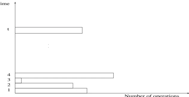
So, an algorithm in the PRAM model

is presented in terms of a sequence of parallel time units (or “rounds”, or “pulses”); we allowpinstructions to be performed at each time unit, one per processor; this means that a time unit consists of a sequence of exactly p instructions to be performed concurrently. See Figure 3

(12)

B(3,1)

B(2,1) B(2,2)

B(1,1) B(1,2) B(1,3) B(1,4)

B(0,1)=A(1) B(0,2)=A(2) B(0,3)=A(3) B(0,4)=A(4) B(0,5)=A(5) B(0,6)=A(6) B(0,7)=A(7) B(0,8)=A(8)

Figure 2: Summation on ann = 8 processor PRAM

Time

. .

p Number of operations 1

2 3 t

Figure 3: Standard PRAM mode: in each of the t steps of an algorithm, exactly p operations, arranged in a sequence, are performed

We refer to such a presentation, as the standard PRAM mode.

The standard PRAM mode has a few drawbacks: (i) It does not reveal how the algorithm will run on PRAMs with different number of processors; specifically, it does not tell to what extent more processors will speed the computation, or fewer processors will slow it. (ii) Fully specifying the allocation of instructions to processors requires a level of detail which might be unnecessary (since a compiler can extract it automatically - see the WD-presentation sufficiency theorem below).

(13)

2.2. Work-Depth presentation of algorithms

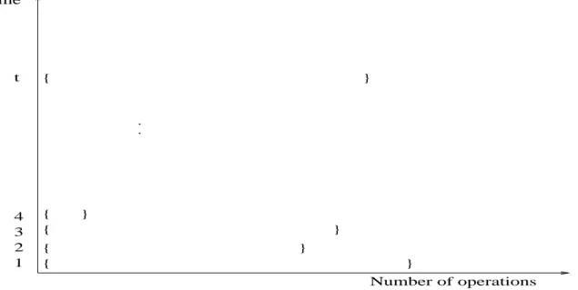
An alternative model which is actually an alternative presentation mode, called Work-Depth, is outlined next. Work-Depth algorithms are also presentedin terms of a sequence of parallel time units (or “rounds”, or “pulses”); however, each time unit consists of a sequence of instructions to be performed concurrently; the sequence of instructions may include any number. See Figure 4.

Number of operations

. .

Time

1 2 3 4 t

Figure 4: WD mode: in each of thetsteps of an algorithm as many operations as needed by the algorithm, arranged in a sequence, are performed

Comment on rigor. Strictly speaking, WD actually defines a slightly different model of computation. Consider an instruction of the form

- for i , 1_≤i_≤α pardo - A(i) := B(C(i))

where the time unit under consideration, consists of a sequence of α concurrent

instruc-tions, for some positive integer α. Models such as Common CRCW WD, Arbitrary

CRCW WD, or Priority CRCW WD, are defined as their PRAM respective counterparts with α processors. We explain below why these WD models are essentially equivalent to their PRAM counterpart and therefore treat the WD only as a separate presentation mode and suppress the fact that these are actually (slightly) different models. The only additional assumption, which we make for proving these equivalences, is as follows. In case the same variable is accessed for both reads and write in the same time unit, all the reads precede all the writes.

The summation example (cont’d). We give a WD presentation for a summation algorithm. It is interesting to note that Algorithm 2, below, highlights the following

(14)

“greedy-parallelism” attribute in the summation algorithm: At each point in time the summation algorithm seeks to break the problem into as many pairwise additions as possible, or, in other words, into the largest possible number of independent tasks that can performed concurrently. We make the same assumptions as for Algorithm 1, above.

ALGORITHM 2 (WD-Summation) 1. for i , 1_≤i_≤n pardo

2. B(0, i) := A(i) 3. for h := 1 to log n

4. for i , 1_≤i_≤n/2h _pardo

5. B(h, i) := B(h₋1,2i₋1) + B(h₋1,2i) 6. for i = 1 pardo output B(log n,1)

The first round of the algorithm (lines 1 and 2) has n operations. The second round (lines 4 and 5 for h= 1) has n/2 operations. The third round (lines 4 and 5 for h= 2) has n/4 operations. In general, the kth round of the algorithm, 1 _≤ k _≤ logn+ 1, has n/2k−1 _{operations and round log}_n _{+ 2 (line 6) has one more operation (note that the use}

of a pardo instruction in line 6 is somewhat artificial). The total number of operations is 2n and the time is logn + 2. We will use this information in the corollary below.

The next theorem demonstrates that the WD presentation mode does not suffer from the same drawbacks as the standard PRAM mode, and that every algorithm in the WD mode can be automatically translated into a PRAM algorithm.

The WD-presentation sufficiency Theorem. Consider an algorithm in the WD mode that takes a total of x =x(n) elementary operations and d=d(n) time. The algorithm can be implemented by anyp=p(n)-processor within O(x/p + d) time, using the same concurrent-write convention as in the WD presentation.

Note that the theorem actually represents five separate theorems for five respective concurrent-read and concurrent-write models: EREW, CREW, Common CRCW, Ar-bitrary CRCW and Priority CRCW.

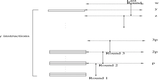
Proof of the Theorem. After explaining the notion of a round-robin simulation, we advance to proving the theorem. Given a sequence of y instructions inst1, . . . , insty, a

round-robin simulation of these instructions by p processors, P1. . . Pp, means the

fol-lowing _⌈y/p_⌉ rounds. See also Figure 5. In round 1, the first group of p instructions inst1. . . instp are performed in parallel, as follows. For each j, 1 ≤j ≤ p, processor Pj

performs instruction instj, respectively. In round 2, the second group of p instructions

instp+1. . . inst2p is performed in parallel, as follows. For each j, 1 ≤ j ≤ p, processor

Pj performs instruction instj+p, respectively. And so on, where in round⌈y/p⌉ (the last

round) some of the processors may stay idle if there are not enough instructions for all of them. The reader can also find a concrete demonstration of this important notion of round-robin simulation in Algorithm 2’ below.

(15)

Round

p 2p 3p y

. . .

. . . . . .

z w

y instructions

Round 1 Round 2

Round 3 Last

Figure 5: Round robin emulation of y instructions by p processors in _⌈y/p_⌉ rounds. In each of the first_⌈y/p_{⌉ −}1 rounds,pinstructions are emulated for a total ofz = p(_⌈y/p_{⌉ −} 1) instructions. In round _⌈y/p_⌉, the remaining y₋z instructions are emulated, each by a processor, while the remaining w₋y processor stay idle, where w = p(_⌈y/p_⌉).

of instructions to be performed by the algorithm at round i. Note that by the definition of x, Pd_i₌₁ xi = x. The p processors can ”simulate” round i of the algorithm in two

stages. In the first stage, only the read instructions of round i are emulated; each read instruction causes storage into a temporary variable. This is done in_⌈xi/p⌉ ≤xi/p + 1

time units, using a round-robin simulation of the xi reads of round i by p processors.

In the second stage, all the other instructions of round i (including write instructions) are performed in additional _⌈xi/p⌉ ≤ xi/p + 1 time units, again using a round-robin

simulations by pprocessors. The theorem follows.

We leave it as an exercise to verify the above proof for the various concurrent-read and concurrent-write models. It can also be readily seen that a converse of the theorem holds true: simply consider a p-processor PRAM algorithm as being in the WD mode, with a sequence ofp instructions at each time unit.

A Corollary (The summation example (cont’d)). As a corollary of the theorem, we conclude that the summation algorithm, Algorithm 2, would run in O(n/p + log n) time on a p-processor PRAM. For p_≤ n/log n, this implies a running time of O(n/p), while for p _≥n/log n, the implied running time is O(log n). Since the algorithm does not involve concurrent reads or writes, thep-processors algorithm can run on an EREW PRAM.

For concreteness, we demonstrate below the spirit of the above proof (of the presentation sufficiency theorem) with respect to Algorithm 2 that was given in the WD-presentation mode. We show how to run it on a p-processor PRAM. Note that, unlike the proof, we emulate the read instructions in the same time unit as other instructions.

(16)

The reader may better appreciate the WD-mode and the WD-presentation sufficiency theorem in view of Algorithm 2’: the theorem saves the need for the tedious effort of manually producing the PRAM-mode.

ALGORITHM 2’ (Summation on a p-processor PRAM)

1. for Pi , 1≤i≤p pardo

2. for j := 1 to _⌈n/p_{⌉ −}1do

- B(0, i + (j ₋1)p) := A(i + (j₋1)p) 3. for i , 1_≤i_≤n ₋ (_⌈n/p_{⌉ −}1)p

- B(0, i + (_⌈n/p_{⌉ −}1)p) := A(i + (_⌈n/p_{⌉ −}1)p) - for i , n ₋ (_⌈n/p_{⌉ −}1)p_≤i_≤p

- stay idle

4. for h := 1 to log n

5. for j := 1 to _⌈n/(2h_p₎_{⌉ −}₁_do _{(*an instruction}_j _{:= 1} _to ₀_do _means:

- “do nothing”*)

- B(h, i+ (j₋1)p) := B(h₋1,2(i+ (j₋1)p)₋1) + B(h₋1,2(i+ (j₋1)p)) 6. for i , 1_≤i_≤n ₋ (_⌈n/(2h_p₎_{⌉ −}₁₎_p

- B(h, i+ (_⌈n/(2h_p₎_{⌉ −}₁₎_p_{) :=} _B₍_h₋₁_,₂₍_i_{+ (}_⌈_n/₍₂h_p₎_{⌉ −}₁₎_p₎₋_{1) +}

- B(h₋1,2(i+ (_⌈n/(2h_p₎_{⌉ −}₁₎_p₎₎

- for i , n ₋ (_⌈n/(2h_p₎_{⌉ −}₁₎_p_≤_i_≤_p

- stay idle

7. for i= 1 output B(log n,1);for i >1 stay idle

Algorithm 2’ simply emulates in a round-robin fashion each sequence of concurrent instruction of Algorithm 2. For instance, lines 1 and 2 in Algorithm 2 have a sequence of n instructions. These instructions are emulated in Algorithm 2’ in_⌈n/p_{⌉ −}1 rounds by line 2, and in an additional round by line 3. The running time of Algorithm 2’ is as follows. Line 2 take _⌈n/p_{⌉ −}1 rounds, and line 3 takes one round, for a total of _⌈n/p_⌉ rounds. The loop for h=k of lines 5-6 takes a total_⌈n/(2h_p₎_⌉ _{rounds. Line 7 takes one}

more round. Summing up the rounds gives

⌈n/p_⌉ + log_Xn

i=1

⌈n/(2hp)_⌉+ 1_≤ log_Xn

i=0

(n/(2hp) + 1) + 1 = O(n/p + logn)

rounds for the PRAM algorithms. This is the same as implied by the WD-presentation sufficiency theorem without going through the hassle of Algorithm 2’.

Measuring the performance of parallel algorithms.

Consider a problem whose input length is n. Given a parallel algorithm in the WD mode for the problem, we can measure its performance in terms of worst-case running time, denotedT(n), and total number of operations, denotedW(n) (where W stands for work). The following are alternative ways for measuring the performance of a parallel algorithm. We have actually shown that they are all asymptotically equivalent.

(17)

1. W(n) operations and T(n) time.

2. P(n) = W(n)/T(n) processors and T(n) time (on a PRAM).

3. W(n)/p time using any number of p_≤W(n)/T(n) processors (on a PRAM). 4. W(n)/p + T(n) time using any number of pprocessors (on a PRAM).

Exercise 1: The above four ways for measuring performance of a parallel algorithms form six pairs. Prove that the pairs are all asymptotically equivalent.

2.3. Goals for Designers of Parallel Algorithms

Our main goal in designing parallel algorithms is efficiency. We intentionally refrain from giving a strict formal definition for when an algorithm is to be considered efficient, but give several informal guidelines.

Consider two parallel algorithms for the same problem. One performs a total of W1(n) operations in T1(n) time and the other performs a total of W2(n) operations in

T2(n) time. Generally, we would like to consider the first algorithm more efficient than the second algorithm if W1(n) = o(W2(n)), regardless of their running times; and if

W1(n) and W2(n) grow asymptotically the same, then the first algorithm is considered more efficient if T1(n) = o(T2(n)). A reason for not giving a categoric definition is the following example. Consider an extreme case where W1(n) = O(n) and T1(n) = O(n), and W2(n) = O(nlogn) and T2(n) = O(logn). It is hard to decide which algorithm is more efficient since the first algorithm needs less work, but the second is much faster. In this case, both algorithms are probably interesting. It is not hard to imagine two users, each interested in different input sizes and in different target machines (i.e., with a different number of processors), where for one user the first algorithm performs better, while for the second user the second algorithm performs better.

Consider a problem, and let T(n) be the best known worst case time upper bound on a serial algorithm for an input of length n.

Assume further that we can prove that this upper bound cannot be asymptotically improved. (Using complexity theory terms, T(n) is the serial time complexity of the problem.) Consider a parallel algorithm for the same problem that performs W(n) op-erations in Tpar(n) time. The parallel algorithm is said to be work-optimal, if W(n)

grows asymptotically the same as T(n). A work-optimal parallel algorithm is work-time-optimal if its running time T(n) cannot be improved by another work-optimal algorithm.

The problem with the definitions above is that often the serial complexity of problems is not known. We see a need to coin a term that will capture the sense of accomplishment for such cases, as well. Assume that we do not know whether T(n) can be improved

(18)

asymptotically, and consider a parallel algorithm for the same problem that performs W(n) work in Tpar(n) time. The parallel algorithm is said to achieve linear speed-up,

ifW(n) grows asymptotically the same asT(n). The problem with this definition is that it may not withstand the test of time: someday, an improved serial algorithm can change the best serial upper bound, and an algorithm that once achieved linear speed-up no longer does that.

Perspective Earlier we used some analogies to serial computation in order to justify the choice of the Work-Depth (or PRAM) model of computation. Still, it is crucial to recognize the following difference between parallel and serial computation in trying to draw further analogies. Serial computing opened the era of computing. To some extent the job was easy because there was no previous computing paradigm that had to be challenged. The situation with parallel computing is different. Serial computing is an enormous success. The problem with this paradigm are as follows: (i) Parallel computing can offer better performance, and (ii) Whether it is already correct to conclude that the serial paradigm has reached a dead-end when it comes to building machines that are much stronger than currently available, or too early, physical and technological limitations suggest that it is just a matter of time till this happens.

2.4. Some final Comments

2.4.1. Default assumption regarding shared assumption access resolution These notes will focus on the the Arbitrary CRCW PRAM and its respective WD model. A partial explanation for this is provided by the following comments regarding the rel-ative power of PRAM models: (1) The Priority CRCW PRAM is most powerful, then come the Arbitrary CRCW PRAM, the Common CRCW PRAM, the CREW PRAM, and finally the EREW PRAM. (2) Some formal simulation results of the most powerful Priority CRCW PRAM on the least powerful EREW PRAM show that the models do not differ substantially. (3) Since all these PRAM models are only virtual models of real machines, a more practical perspective is to compare their emulations on a possible target machine. It turns out that the models differ even less from this perspective. In view of the above points, it remains to justify the choice of the Arbitrary CRCW PRAM over the stronger Priority CRCW PRAM. The reason is that its implementation considerations favor relaxing the order in which concurrent operations can be performed. The home page for the UMD PRAM-On-Chip project provides more information.

2.4.2. NC: A Related, Yet Different, Efficiency Goal In stating the goals for parallel computing, one has to remember that its primary objective is to challenge the supremacy of serial computing. For this reason, our definitions of either linear speed-up or optimal speed-up are very sensitive to relationship between a parallel algorithm and its the serial alternative. The theoretical parallel computing literature had been motivated

(19)

by other goals as well. A complexity theory approach, which opined that “a problem is amenable to parallel computing if it can be solved in poly-logarithmic time using a polynomial number of processors”, has received a lot of attention in the literature. Such problems are widely known as the class NC, or Nick’s Class, in honor of Nick Pippenger). This complexity theory approach is of fundamental importance: for instance, if one shows that a problem is “log-space complete for P” then the problem is unlikely to be in the class NC - a very useful insight. Therefore, a next step, beyond these notes, for a reader who wants to know more about parallel algorithms, will have to include learning the basic concepts of this theory.

2.4.3. On selection of material for these notes The goal of these notes is to familiarize the reader with the elementary routines, techniques and paradigms in the current knowledge base on parallel algorithm. In planning these notes, we were guided by the following two principles.

The first principle is actually a compromise between two conflicting approaches: (1) “Breadth-first search”: Present the theory as a “bag of tricks”, describing one trick at a time. Assuming that the curriculum can allocate only a limited time to the topics covered in these notes, this will maximize the number of tricks learned at the expense of not exposing the reader to more involved parallel algorithms. However, since designing parallel algorithms may be a rather involved task, an important aspect may be missed by this approach. This brings us to the second approach. (2) “Depth-first search”: Present in full a few relatively involved parallel algorithms.

Thesecond principle applies a“prefix rule of thumb”. At each point, we tried to evaluate what would be the next most important thing that the reader should know assuming that he/she has time to learn only one more section. These two principles may explain to the more knowledgeable reader our selection of material.

2.4.4. Level of material I taught this material on several occasions to beginning graduate students; recently, undergraduates were allowed to take the course as an elective and constituted a considerable fraction of the class. The first ten sections (i.e., everything excluding the section on graph connectivity) were taught in 21 lecture hours, where a lecture hour is defined as 50 minutes net time of teaching. My impression is that this material is suitable for undergraduate computer science students in their junior or senior year, and can cover about a half of an undergraduate course. This can be combined into a full course with another topic for the remaining part of the course. Another option is to teach next the connectivity section, which took the author 6-7 more hours. Together with some additional material (e.g., introduction to parallel computing, or even introduction to NP-Completeness) this can make a junior or senior level undergraduate course or a beginning graduate course.

(20)

3. Technique: Balanced Binary Trees; Problem: Prefix-Sums

Parallel prefix-sums might be the most heavily used routine in parallel algorithms. We already saw how balanced binary trees are used in a parallel summation algorithm. This section demonstrates a slightly more involved use of balanced binary trees.

The prefix-sums problem

Input: An array A of n elements drawn from some domain. Assume that a binary

operation, denoted _∗, is defined on the set. Assume also that _∗ is associative; namely, for any elements a, b, c in the set, a_∗(b_∗c) = (a_∗b)_∗c.

(The operation_∗ is pronounced “star” and often referred to as “sum” because addition, relative to real numbers, is a common example for _∗.)

The n prefix-sums of array A are defined asPi

j=1A(j), fori, 1≤i≤n, or:

A(1)

A(1)_∗A(2) . . .

A(1)_∗A(2)_∗. . ._∗A(i) . . .

A(1)_∗A(2)_∗ . . . _∗A(n)

The prefix sums algorithm below assumes that n = 2k _{for some integer} _k_{, and that}

the arrays B(h, i) and C(h, i) for 0_≤ h _≤logn and 1_≤ i _≤n/2h_{, are given for storing}

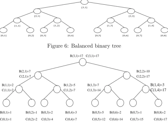
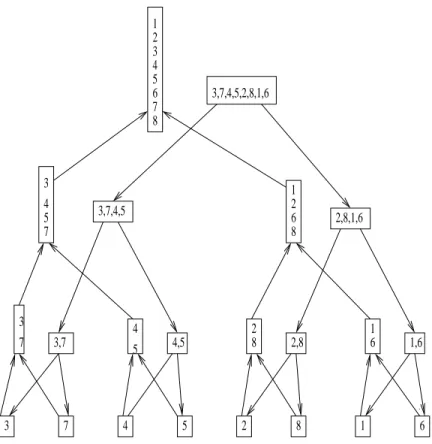
intermediate steps of the computation. The algorithm works in two stages each taking logarithmic time. The first stage (lines 1-3 below) is similar to the summation algorithm of the previous section, where the computation advances from the leaves of a balanced binary tree to the root and computes, for each internal node [h, i] of the tree, the sum of its descendant leaves into B(h, i). The second stage (lines 4-7 below) advances in the opposite direction, from the root to the leaves. For each internal node [h, i] the prefix sum of its rightmost leaf is entered into C(h, i). Namely, C(h, i) is the prefix-sum A(1)_∗A(2)_∗. . ._∗A(α), where [0, α] is the rightmost descendant leaf of [h, i]. In particular, C(0,1), C(0,2), . . . , C(0, n) have the desired prefix-sums. Figure 6 describes the B and C arrays, and the drilling example below. describes a balanced binary tree, Figure 7.

(21)

[0,1] [0,2] [0,3] [0,4] [0,5] [0,6] [0,7] [0,8]

[2,1] [2,2]

[3,1]

[1,1] [1,2] [1,3] [1,4]

Figure 6: Balanced binary tree

C(1,4)=17 B(1,4)=3

B(0,2)=1 B(0,3)=2 B(0,7)=1 B(0,8)=2 B(1,2)=5

B(1,1)=2

B(3,1)=17 C(3,1)=17

C(2,2)=17 B(2,2)=10

C(0,2)=2 C(0,3)=4 C(0,4)=7 C(0,5)=12 C(0,8)=17 C(1,3)=14

C(1,2)=7 C(2,1)=7

B(0,4)=3 B(0,5)=5 B(1,3)=7

B(0,6)=2

C(0,6)=14 C(0,7)=15 B(2,1)=7

B(0,1)=1 C(0,1)=1 C(1,1)=2

Figure 7: The prefix-sums algorithm

ALGORITHM 1 (Prefix-sums) 1. for i , 1_≤i_≤n pardo

- B(0, i) := A(i) 2. for h := 1 to log n

3. for i , 1_≤i_≤n/2h _pardo

- B(h, i) := B(h₋1,2i₋1) _∗ B(h₋1,2i) 4. for h := logn to 0

5. for i even, 1 _≤i_≤n/2h _pardo

- C(h, i) := C(h+ 1, i/2) 6. for i= 1 pardo

- C(h,1) := B(h,1)

7. for i odd, 3_≤i_≤n/2h _pardo

- C(h, i) := C(h+ 1,(i₋1)/2) _∗ B(h, i) 8. for i , 1_≤i_≤n pardo

(22)

A drilling example. Let us run Algorithm 1 on the following instance. See also Figure 7. n = 8 and A = 1,1,2,3,5,2,1,2 and _∗ is the + operation. Line 1 implies B(0; 1. . .8) = 1,1,2,3,5,2,1,2. Lines 2-3 imply: B(1; 1,2,3,4) = 2,5,7,3 for h= 1, B(2; 1,2) = 7,10 forh= 2, andB(3,1) = 17 forh= 3. Lines 4-7 implyC(3,1) = 17 for h = 3, C(2; 1,2) = 7,17 for h = 2, C(1; 1,2,3,4) = 2,7,14,17 for h = 1, and finally C(0; 1. . .8) = 1,2,4,7,12,14,15,17 for h= 0.

Complexity. The operations of the prefix-sums algorithm can be “charged” to nodes of the balanced binary tree, so that no node will be charged by more than a constant number of operations. These charges can be done as follows. For each assignment into either B(h, i) or C(h, i), the operations that led to it are charged to node [i, j]. Since the number of nodes of the tree is 2n₋1, W(n), the total number of operations of the algorithm isO(n). The time isO(logn) since it is dominated by the loops of lines 2 and 4, each requiring logn rounds.

Theorem 3.1: The prefix-sums algorithm runs in O(n) work and O(logn)time.

3.1. Application - the Compaction Problem

We already mentioned that the prefix-sums routine is heavily used in parallel algorithms. One trivial application, which is needed later in these notes, follows:

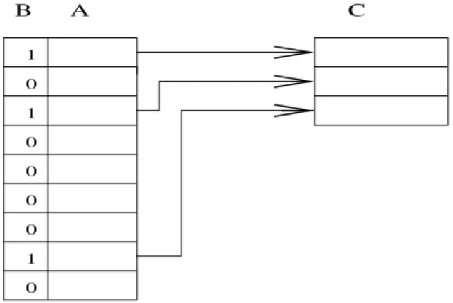
Input. An array A = A(1), . . . , A(n) of (any kind of) elements and another array B = B(1), . . . , B(n) of bits (each valued zero or one).

Thecompactionproblem is to find a one-to-one mapping from the subset of elements of A(i), for whichB(i) = 1, 1_≤i_≤n, to the sequence (1,2, . . . , s), wheresis the (a priori unknown) numbers of ones in B. Below we assume that the mapping should be order preserving. That is, if A(i) is mapped to k and A(j) is mapped to k+ 1 then i < j. However, quite a few applications of compaction do not need to be order preserving.

For computing this mapping, simply compute all prefix sums with respect to array B. Consider an entry B(i) = 1. If the prefix sum ofiis j then map A(i) into j. See also Figure 8.

Theorem 3.2: The compaction algorithm runs inO(n) work and O(logn) time.

Exercise 2: Let A be a memory address in the shared memory of a PRAM. Suppose

that all p processors of the PRAM need to “know” the value stored in A. Give a fast

EREW algorithm forbroadcastingthe value of Ato allpprocessors. How much time will

this take?

Exercise 3: The minimum problem is defined as follows. Input: An array A of n ele-ments drawn from some totally ordered set. The minimum problem is to find the smallest

(23)

B A C 1

0 1 0 0 0 0 1 0

Figure 8: Application of prefix-sums for compaction

element in array A.

(1) Give an EREW PRAM algorithm that runs in O(n) work and O(logn) time for the

problem.

(2) Suppose we are given only p_≤n/logn processors, which are numbered from1 top.

For the algorithm of item (1) above, describe the algorithm to be executed by processor

i, 1_≤i_≤p.

The prefix-minproblem has the same input as for the minimum problem and we need to find for each i, 1_≤i_≤n, the smallest element among A(1), A(2), . . . , A(i).

problem.

Exercise 4: The nearest-one problem is defined as follows. Input: An array A of size n

of bits; namely, the value of each entry ofA is either 0 or1. The nearest-one problem is to find for each i, 1_≤i_≤n, the largest index j _≤i, such thatA(j) = 1.

problem.

The input for the segmented prefix-sums problem includes the same binary array A as

above, and in addition an array B of size n of numbers. The segmented prefix-sums

problem is to find for each i, 1 _≤i_≤n, the sum B(j) +B(j + 1) +. . .+B(i), where j

is the nearest-one for i(if i has no nearest-one we define its nearest-one to be 1).

(2) Give an EREW PRAM algorithm for the problem that runs inO(n)work andO(logn)

time.

3.2. Recursive Presentation of the Prefix-Sums Algorithm

Recursive presentations are useful for describing serial algorithms. They are also useful for describing parallel ones. Sometimes they play a special role in shedding new light on a technique being used.

(24)

The input for the recursive procedure is an array (x1, x2, . . . , xm) and the output is

given in another array (u1, u2, . . . , um). We assume that log2m is a non-negative integer. PREFIX-SUMS(x1, x2, . . . , xm;u1, u2, . . . , um)

1. if m= 1 then u1 := x1; exit 2. for i, 1_≤i_≤m/2 pardo - yi := x2i−1∗x2i

3. PREFIX-SUMS(y1, y2, . . . , ym/2;v1, v2, . . . , vm/2) 4. for i even, 1_≤i_≤m pardo

- ui := vi/2

5. for i= 1 pardo

- u1 := x1

6. for i odd, 3_≤i_≤m pardo - ui := v(i−1)/2∗xi

The prefix-sums algorithm is started by the following routine call: PREFIX-SUMS(A(1), A(2), . . . , A(n);C(0,1), C(0,2), . . . , C(0, n)).

The complexity analysis implied by this recursive presentation is rather concise and elegant. The time required by the routine PREFIX-SUMS, excluding the recursive call in instruction 3, isO(1), or_≤α, for some positive constantα. The number of operations required by the routine, excluding the recursive call in instruction 3, is O(m), or _≤βm, for some positive constant β. Since the recursive call is for a problem of size m/2, the running time, T(n), and the total number of operations, W(n), satisfy the recurrences:

T(n)_≤T(n/2) + α W(n)_≤W(n/2) + βn Their solutions areT(n) = O(logn), andW(n) = O(n).

Exercise 5: Multiplying two n_×n matrices A and B results in another n_×n matrix

C, whose elements ci,j satisfy ci,j = Pnk=1ai,kbk,j.

(1) Given two such matrices A and B, show how to compute matrix C inO(logn) time

using n3 _processors.

(2) Suppose we are given only p _≤ n3 _{processors, which are numbered from} ₁ _to _p_.

Describe the algorithm of item (1) above to be executed by processor i, 1_≤i_≤p.

(3) In case your algorithm for item (1) above required more than O(n3₎ _{work, show how}

to improve its work complexity to get matrix C in O(n3₎ _{work and} _O_(log_n₎ _time.

(4) Suppose we are given onlyp_≤n3_/_log_n _{processors, which are numbered from}₁_to_p_.

(25)

4. The Simple Merging-Sorting Cluster

In this section we present two simple algorithmic paradigms called: partitioning and divide-and-conquer. Our main reason for considering the problems of merging and sorting in this section is for demonstrating these paradigms.

4.1. Technique: Partitioning; Problem: Merging

Input: Two arraysA = A(1). . . A(n) and B = B(1). . . B(m) consisting of elements drawn from a totally ordered domain S. We assume that each array is monotonically non-decreasing.

The merging problem is to map each of these elements into an array

C = C(1). . . C(n+m) which is also monotonically non-decreasing.

For simplicity, we will assume that: (i) the elements of A and B are pairwise distinct, (ii) n = m, and (iii) both logn and n/logn are integers. Extending the algorithm to cases where some or all of these assumptions do not hold is left as an exercise.

It turns out that a very simple divide-and-conquer approach, which we call parti-tioning, enables to obtain an efficient parallel algorithm for the problem. An outline of the paradigm follows by rephrasing the merging problem as a ranking problem, for which three algorithms are presented. The first algorithm is parallel and is called a “surplus-log” algorithm. The second is a standard serial algorithm. The third algorithm is the parallel merging algorithm. Guided by the partitioning paradigm, the third and final algorithm uses the first and second algorithms as building blocks.

The partitioning paradigm Let n denote the size of the input for a problem. In-formally, a partitioning paradigm for designing a parallel algorithm could consist of the following two stages:

partitioning - partition the input into a large number, say p, of independent small jobs, so that the size of the largest small job is roughly n/p, and

actual work - do the small jobs concurrently, using a separate (possibly serial) algo-rithm for each.

A sometimes subtle issue in applying this simple paradigm is in bringing about the lowest upper bound possible on the size of any of the jobs to be done in parallel.

The merging problem can be rephrased as a ranking problem, as follows. Let

B(j) = z be an element of B, which is not in A. Then RANK(j, A) is defined to be i if A(i) < z < A(i + 1), for 1 _≤ i < n; RANK(j, A) = 0 if z < A(1) and RANK(j, A) = n if z > A(n). The ranking problem, denoted RANK(A, B) is to compute: (i)RANK(i, B) (namely, to rank element A(i) inB), for every 1_≤i_≤n, and

(26)

(ii) RANK(i, A) for every 1_≤i_≤n.

Claim. Given a solution to the ranking problem, the merging problem can be solved in constant time and linear work. (Namely in O(1) time andO(n+m) work.)

To see this, observe that element A(i), 1 _≤ i _≤ n should appear in location i + RANK(i, B) of the merged array C. That is, given a solution to the ranking problem, the following instructions extend it into a solution for the merging problem: for 1_≤i_≤n pardo

- C(i + RANK(i, B)) := A(i) for 1_≤i_≤n pardo

- C(i + RANK(i, A)) := B(i)

It is now easy to see that the Claim follows. This allows devoting the remainder of this section to the ranking problem.

Our first “surplus-log” parallel algorithm for the ranking problem works as fol-lows.

for 1_≤i_≤n pardo

- Compute RANK(i, B) using the standard binary search method. - Compute RANK(i, A) using binary search

For completeness, we describe the binary search method. The goal is to compute RANK(i, B) whereB = B(1, . . . , n). Binary search is a recursive method. Assume be-low thatx = _⌈n/2_⌉. ElementB(x) is called themiddleelement ofB. Now,RANK(i, B) is computed recursively as follows.

if n= 1

then if A(i)< B(1)then RANK(i, B) := 0 else RANK(i, B) := 1 else

- if A(i)< B(x) then RANK(i, B) := RANK(i, B(1, . . . , x₋1)) - if A(i)> B(x) then RANK(i, B) := x + RANK(i, B(x+ 1, . . . , n))

Binary search takes O(logn) time. The above surplus-log parallel algorithm for the ranking problem takes a total ofO(nlogn) work andO(logn) time. The namesurplus-log highlights the O(nlogn), instead of O(n), bound for work.

A serial routine for the ranking problem follows. Since it will be used later with n₆=m, we differentiate the two values in the routine below.

SERIAL₋RANK(A(1), A(2), . . . , A(n);B(1), B(2), . . . , B(m))

k := 0 andl := 0; add two auxiliary elementsA(n+ 1) and B(m+ 1) which are each larger than both A(n) and B(m)

while k _≤n orl _≤m do - if A(k+ 1)< B(l+ 1)

- then RANK(k+ 1, B) := l; k := k+ 1 - else RANK(l+ 1, A) := k; l := l+ 1

In words, starting from A(1) and B(1), in each round one element from A is compared with one element ofB and the rank of the smaller among them is determined. SERIAL₋

(27)

RANK takes a total ofO(n+m) time.

We are ready to present the parallel algorithm for ranking. For simplicity, we assume again thatn=mand thatA(n+ 1) andB(n+ 1) are each larger than both A(n) and B(n).

Stage 1 (partitioning). Let x = n/logn. We use a variant of the surplus-log algo-rithm for the purpose of partitioning the original ranking problem into O(x) problems.

1.1 We select x elements of A and copy them into a new array A SELECT. The x

elements are selected so as to partition A into x (roughly) equal blocks. Specifically, A SELECT = A(1), A(1 + logn), A(1 + 2 logn). . . A(n + 1 ₋ logn). For each A SELECT(i), 1 _≤ i _≤ x separately (and in parallel), compute RANK(i, B) using binary search in O(logn) time. (Note: It should be clear from the context that i is an index in array A SELECT and not array A.)

1.2 Similarly, we select x elements of B, and copy them into a new array

B SELECT. Thexelements partition B intop(roughly) equal blocks: B SELECT = B(1), B(1 + logn), B(1 + 2 logn). . . B(n+ 1₋logn). For each B SELECT(i), 1_≤ i _≤ x separately, compute RANK(i, A) using binary search in O(logn) time; i is an index in array B SELECT.

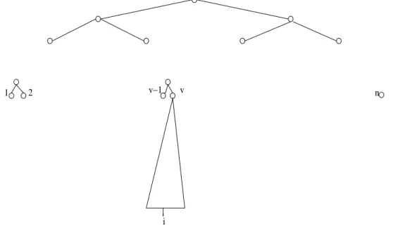
The situation following the above computation is illustrated in Figure 9.

High-level description of Stage 2. The original ranking problem was partitioned in Stage 1 into 2n/logn “small ranking problems”. The ranking of each non-selected element ofAandBis determined in Stage 2 byexactly onesmall problem. Importantly, the size of each small problem does not exceed 2 logn. This allows solving in parallel all small problems, where each will be solved in O(logn) time using SERIAL₋RANK.

Each element A SELECT(i) and B SELECT(i), 1_≤i _≤n/logn, defines a small ranking problem of those elements in A and B which are just larger than itself. Specifi-cally:

Stage 2(a) (actual ranking for the small problems ofA SELECT(1, . . . , n/logn). Let A SELECT(i), for some i, 1 _≤ i _≤ n/logn. The input of the ranking problem of A SELECT(i) consists of two subarrays: (i) the successive subarray of A that spans between element (i ₋1) logn + 1, denoted a₋ start₋a(i), and some element de-noted a₋end₋a(i), and (ii) the successive subarray of B that spans between element a₋start₋b(i) = RANK(i, B) + 1 (i is an index of A SELECT) and some element a₋end₋b(i). Rather than showing how to finda₋end₋a(i) anda₋end₋b(i), we show how to determine that SERIAL₋RANK has completed its “small ranking problem”. As the comparisons between elements of A and B proceed, this determination is made upon the first comparison in which another element of A SELECT or B SELECT (or A(n+ 1) or B(n+ 1)) “loses”. The rationale being that that this comparison already belongs to the next small problem.

Stage 2(b) (actual ranking for the small problems ofB SELECT(1, . . . , n/logn). The input of the problems defined by an elementB SELECT(i), 1_≤i_≤n/logn, con-sists of: (i) the successive subarray of B that spans between element (i₋1) logn + 1,

(28)

4 6 8 9 16 17 18 19 20 21 23 25 27 29 31 32 1 2 3 5 7 10 11 12 13 14 15 22 24 26 28 30 6 8 9 17 18 19 21 23 25 29 31 32 2 3 5 10 11 12 14 15 26 28 30 22

A

B

_A

_B

Step 2

actual work

Step 1

partitioning

Figure 9: Main steps of the ranking/merging algorithm

denoted b₋start₋b(i), and some element denoted b₋end₋b(i), and (ii) the succes-sive subarray of A that spans between element b₋start₋a(i) = RANK(i, A) + 1 (i is an index of B SELECT) and some element b ₋end ₋a(i). Determining that SERIAL₋RANK has completed its small ranking problem is similar to case (a) above. Complexity. Stage 1 takesO(xlogn) work andO(logn) time, which translates into O(n) work and O(logn) time. Since the input for each of the 2n/logn small ranking problems contains at most logn elements from array Aand at most logn elements from array B, Stage 2 employs O(n/logn) serial algorithms, each takes O(logn) time. The total work is, therefore, O(n) and the time is O(logn).

Theorem 4.1: The merging/ranking algorithm runs inO(n)work and O(logn) time.

Exercise 6: Consider the merging problem as stated in this section. Consider a variant

(29)

positive integer between 1and n. Describe the resulting merging algorithm and analyze

its time and work complexity as a function of both x and n.

Exercise 7: Consider the merging problem as stated in this section, and assume that the values of the input elements are not pairwise distinct. Adapt the merging algorithm for this problem, so that it will take the same work and the same running time.

Exercise 8: Consider the merging problem as above, and assume that the values of n

and m are not equal. Adapt the merging algorithm for this problem. What are the new

work and time complexities?

Exercise 9: Consider the merging algorithm presented in this section. Suppose that the algorithm needs to be programmed using the smallest number of Spawn commands in an XMT-C single-program multiple-data (SPMD) program. What is the smallest number of Spawn commands possible? Justify your answer.

(Note: This exercise should be given only after XMT-C programming has been intro-duced.)

4.2. Technique: Divide and Conquer; Problem: Sorting-by-merging

Divide and conquer is a useful paradigm for designing serial algorithms. Below, we show that it can also be useful for designing a parallel algorithm for the sorting prob-lem.

Input: An array of n elements A = A(1), . . . , A(n), drawn from a totally ordered domain.

The sorting problem is to reorder (permute) the elements of A into an array

B = B(1), . . . , B(n), such that B(1)_≤B(2)_≤. . ._≤B(n).

Sorting-by-merging is a classic serial algorithm. This section demonstrates that some-times a serial algorithm translates directly into a reasonably efficient parallel algorithm. A recursive description follows.

MERGE ₋SORT(A(1), A(2), . . . , A(n);B(1), B(2), . . . , B(n)) Assume that n= 2l _{for some integer} _l _≥₀

if n = 1

then return B(1) :=A(1)

else call, in parallel, MERGE₋SORT(A(1), . . . , A(n/2);C(1), . . . C(n/2)) and - MERGE₋SORT(A(n/2 + 1), . . . , A(n);C(n/2 + 1), . . . , C(n))

- Merge C(1), . . . C(n/2)) andC(n/2 + 1), . . . , C(n)) into B(1), B(2), . . . , B(n))

(30)

4 5

7 4 5 2 8 1 6

3,7 4,5

2

8 2,8 1,6

1 6 3

5 7 4

2,8,1,6 1

2 8 6 3,7,4,5,2,8,1,6 1

2 4 5 6 7 8 3

3 3 7

3,7,4,5

Figure 10: Example of the merge-sort algorithm

A = (3,7,4,5,2,8,1,6). The eight elements are repeatedly split into two sets till singleton sets are obtained; in the figure, move downwards as this process progresses. The single elements are then repeatedly pairwise merged till the original eight elements are sorted; in the figure, move upwards as this process progresses.

Complexity. The merging algorithm of the previous section runs in logarithmic time and linear work. Hence, the time and work of merge-sort satisfies the following recurrence inequalities:

T(n)_≤T(n/2) + αlogn; W(n)_≤2W(n/2) + βn

where α, β > 0 are constants. The solutions are T(n) = O(log2n) and

W(n) = O(nlogn).

Theorem 4.2: Merge-sort runs in O(nlogn) work and O(log2n)time.

Similar to the prefix-sums algorithm above, the merge-sort algorithm could have also been classified as a “balanced binary tree” algorithm. In order to see the connection, try to give a non-recursive description of merge-sort.

(31)

5. “Putting Things Together” - a First Example. Techniques:

Informal Work-Depth (IWD), and Accelerating Cascades;

Problem: Selection

One of the biggest challenges in designing parallel algorithms is overall planning (“macro-design”). In this section, we will learn two macro-techniques: (1) Accelerating Cascades provides a way for taking several parallel algorithms for a given problem and deriving out of them a parallel algorithm, which is more efficient than any of them separately; and (2) Informal Work-Depth (IWD) is a description methodology for parallel algorithm. The methodology guides algorithm designers to: (i) focus on the most crucial aspects of a parallel algorithm, while suppressing a considerable number of significant details, and (ii) add these missing details at a later stage. IWD frees the parallel algorithm designers to devote undivided attention to achieving the best work and time. The experience and training acquired through these notes provide the skills for filling in the missing details at a later stage. Overall, this improves the effectiveness of parallel algorithm design. In this section, we demonstrate these techniques for designing a fast parallel algorithm that needs onlyO(n) work for the selection problem.

The selection problem

Input: An array A = A(1), A(2), . . . , A(n) ofn elements drawn from a totally ordered domain, and an integer k, 1_≤k _≤n.

An element A(j) is ak-th smallest element ofAif at mostk₋1 elements ofAare smaller and at mostn₋k elements are larger. Formally,_|{i:A(i)< A(j)f or1_≤i_≤n_{}| ≤}k₋1 and _|{i:A(i)> A(j)f or 1_≤i_≤n_{}| ≤}n₋k.

The selection problem is to find a k-th smallest element of A.

Example. Let A = 9,7,2,3,8,5,7,4,2,3,5,6 be an array of 12 integers, and let k = 4. Then, each among A(4) and A(10) (whose value is 3) is a 4-th smallest element of A. Fork = 5, A(8) = 4 is the only 5-th smallest element.

The selection problem has several notable instances: (i) for k = 1 the selection problem becomes the problem of finding the minimum element in A, (ii) for k = n the selection problem becomes the problem of finding the maximum element inA, and (iii) for k =_⌈n/2_⌉ the k-smallest element is themedianof A and the selection problem amounts to finding this median.

5.1. Accelerating Cascades

For devising the fast O(n)-work algorithm for the selection problem, we will use two building blocks. Each building block is itself an algorithm for the problem:

(1) Algorithm 1 works in O(logn) iterations. Each iteration takes an instance of the selection problem of size m and reduces it in O(logm) time and O(m) work to another instance of the selection problem whose size is bounded by a fraction of m (specifically,

(32)

≤3m/4). Concluding that the total running time of such an algorithm is O(log2n) and its total work is O(n) is easy.

(2) Algorithm 2 runs in O(logn) time and O(nlogn) work.

The advantage of Algorithm 1 is that it needs only O(n) work, while the advantage of Algorithm 2 is that it requires less time. The accelerating cascades technique gives a way for combining these algorithms into a single algorithm that is both fast and needs O(n) work. The main idea is to start with Algorithm 1, but, instead of running it to completion, switch to Algorithm 2. This is demonstrated next.

An ultra-high-level description of the selection algorithm

Step 1. Apply Algorithm 1 forO(log logn) rounds to reduce an original instance of the selection problem into an instance of size _≤n/logn.

Step 2. Apply Algorithm 2.

Complexity analysis. We first confirm thatr = O(log logn) rounds are sufficient to bring the size of the problem below n/logn. To get (3/4)r_n _≤ _n/_log_n_{, we need}

(4/3)r _≥ _log_n_{. The smallest value of} _r _{for which this holds is log}

4/3logn. This is indeed O(log logn). So, Step 1 takes O(lognlog logn) time. The number of operations is Pr−1

i=0(3/4)in = O(n). Step 2 takes additional O(logn) time and O(n) work. So, in total, we get O(lognlog logn) time, andO(n) work.

Following this illustration of the accelerating cascades technique, we proceed to present the general technique.

The Accelerating Cascades Technique

Consider the following situation: for a given problem of size n we have two parallel algorithms. Algorithm A performs W1(n) operations in T1(n) time, and Algorithm B performs W2(n) operations in T2(n) time. Suppose that Algorithm A is more efficient (W1(n) < W2(n)), while Algorithm B is faster (T1(n) < T2(n) ). Assume also that Algorithm A is a “reducing algorithm” in the following sense. Given a problem of size n, Algorithm A operates in phases where the output of each successive phase is a smaller instance of the problem. The accelerating cascades technique composes a new algorithm out of algorithms A and B, as follows. Start by applying Algorithm A. Once the output size of a phase of this algorithm is below some threshold, finish by switching to Algorithm B. It is easy to see from the ultra-high-level description of the selection algorithm that it indeed demonstrates the accelerating cascades technique. It is, of course, possible that instead of the first algorithm there will be a chain of several reducing algorithms with increasing work and decreasing running times. The composed algorithm will start with the slowest (and most work-efficient) reducing algorithm, switch to the second-slowest (and second most work-efficient) reducing algorithm, and so on, until the fastest and least work-efficient reducing algorithm. Finally, it will switch to the last algorithm which need not be a reducing one.

Remark The accelerating cascades framework permits the following kind of budget considerations in the design of parallel algorithms and programs. Given a “budget” for