OF MENU COST MODELS∗ EMINAKAMURA ANDJ ´ONSTEINSSON
We establish five facts about prices in the U.S. economy: (1) For consumer prices, the median frequency of nonsale price change is roughly half of what it is including sales (9–12% per month versus 19–20% per month for identical items; 11–13% per month versus 21–22% per month including product substitutions). The median frequency of price change for finished-goods producer prices is comparable to that of consumer prices excluding sales. (2) One-third of nonsale price changes are price decreases. (3) The frequency of price increases covaries strongly with inflation, whereas the frequency of price decreases and the size of price increases and price decreases do not. (4) The frequency of price change is highly seasonal: it is highest in the first quarter and then declines. (5) We find no evidence of upward-sloping hazard functions of price changes for individual products. We show that the first, second, and third facts are consistent with a benchmark menu-cost model, whereas the fourth and fifth facts are not.
I. INTRODUCTION
The nature of price setting has important implications for a range of issues in macroeconomics, including the welfare conse-quences of business cycles, the behavior of real exchange rates, and optimal monetary policy. We use Bureau of Labor Statistics (BLS) microdata underlying the consumer and producer price dices to document five basic features of price adjustment. We in-terpret this evidence through the lens of a benchmark menu cost model.
We begin by estimating the frequency of price change. Until recently, the best sources of information on U.S. pricing behavior were studies of price adjustment for particular products (Cecchetti 1986; Kashyap 1995), broader surveys of firm managers (Blinder et al. 1998), and evidence on the dynamics of industrial prices (Carlton 1986). The conventional wisdom from this literature was
∗We would like to thank Robert Barro for invaluable advice and encour-agement. We would like to thank Daniel Benjamin, David Berger, Leon Berkel-mans, Craig Brown, Charles Carlstrom, Gary Chamberlain, Tim Erickson, Mark Gertler, Mike Golosov, Gita Gopinath, Teague Ruder, Oleksiy Kryvtsov, Gregory Kurtzon, Robert McClelland, Greg Mankiw, Ariel Pakes, Ricardo Reis, Roberto Rigobon, John Rogers, Ken Rogoff, Philippa Scott, Aleh Tsyvinsky, Randal Ver-brugge, Michael Woodford, seminar participants at various institutions as well as our editor, Larry Katz, and anonymous referees for helpful comments and discus-sions. We particularly want to thank Mark Bils and Pete Klenow for thoughtful and inspiring conversations. We are grateful to Martin Feldstein for helping us obtain access to the data; without his help this work would not have been possible. We are grateful to the Warburg Fund at Harvard University for financial support.
C
2008 by the President and Fellows of Harvard College and the Massachusetts Institute of Technology.
The Quarterly Journal of Economics, November 2008
that prices adjusted on average once a year. Bils and Klenow (2004) dramatically altered this conventional wisdom by showing that the median frequency of price change for nonshelter con-sumer prices in 1995–1997 was 21%, implying a median duration of 4.3 months.
We use a substantially more detailed data set than Bils and Klenow (2004) that contains the micro-level price data underlying the nonshelter component of the Consumer Price Index (CPI).1
This data set has been used by Hosken and Reiffen (2007, 2004) and Klenow and Kryvtsov (2008) to analyze price adjustment behavior. We find that temporary sales play an important role in generating price flexibility for retail prices in categories that account for about 40% of nonshelter consumer expenditures. Whereas the median frequency of price change including sales is 19%–20% per month, we find that the median frequency of nonsale price change for identical items is only 9%–12% per month depending on the time period and how we treat nonsale price changes over the course of sales and stockouts.
Our estimates of the median frequency of price change for identical items may be inverted to obtain estimates of the me-dian duration of regular prices. Excluding product substitutions, these frequency estimates imply uncensored durations of regular prices of between 8 and 11 months. Yet, substitutions often trun-cate regular price spells. If we include price changes associated with product substitutions, the median frequency of nonsale price change increases by between 1 and 2 percentage points. This im-plies median durations until either the regular price changes or the product disappears at between 7 and 9 months.
The importance of temporary sales—and to a lesser extent substitutions—in generating price changes in the U.S. data draws attention to the question of whether the relative frequency of dif-ferent types of price changes is an important determinant of the macroeconomic implications of price rigidity. In other words: “Is a price change just a price change?” An important lesson from the theoretical literature on price adjustment is that different types of price adjustments can have strikingly different macroeconomic
1. Bils and Klenow (2004) used the BLS Commodities and Services Substitu-tion Rate Table for 1995–1997. This data set contains average frequencies of price changes and substitutions by disaggregated product categories over the 1995– 1997 period. In contrast, the CPI research database contains the actual data se-ries on prices underlying the Consumer Price Index for the 1988–2005 period. See Section II for a more detailed discussion of the data.
implications. For example, the Calvo (1983) model and the Caplin and Spulber (1987) model have very different macroeconomic im-plications for the same frequency of price change.
For this reason, an important focus of this paper is to docu-ment and contrast the empirical characteristics of the different types of price changes observed in U.S. consumer data. First, we document that sale price changes display markedly different em-pirical features than regular price changes. Sale price changes are much more transient than regular price changes; and in most cases where a price is observed before and after a sale, the price returns to its original level following the sale.
There are a number of reasons why it may be important to distinguish between sale and nonsale price changes. First, the transience of price adjustment associated with sales implies that a given number of price changes due to sales yield much less aggregate price adjustment than the same number of regular price changes (Kehoe and Midrigan 2007). Second, some types of sales may be orthogonal to macroeconomic conditions. Third, transitory sales are a much more pervasive phenomenon in retail prices than in wholesale prices, implying that temporary sales may be less responsive to shocks at the wholesale than at the retail level of production.
Price changes due to product substitutions are a second class of price changes that we argue is fundamentally different from the regular price changes typically emphasized by macroeconomists. This source of price flexibility is particularly important for durable goods. For example, the spring and fall clothing seasons in apparel and the new model year for cars are associated with a large num-ber of price changes due to the introduction of new products. Many factors other than a firm’s desire to change its price influence its decision to introduce a new product. The theoretical literature on price adjustment has shown that price changes that are mo-tivated primarily by a large difference between a firm’s current price and its desired price yield much greater aggregate price flexibility than those that are motivated by other factors (Caplin and Spulber 1987; Golosov and Lucas 2007). In state-dependent pricing models, it is therefore crucial to treat product substitu-tions separately from other types of price changes (Nakamura and Steinsson 2007). In contrast, time-dependent pricing models should arguably be calibrated to the frequency of price change including substitutions because in these models the timing ofall
We also present the first broad-based evidence on U.S. price dynamics at the producer level. To study this issue, we created a new data set on producer prices from the production files used by the BLS to construct the Producer Price Index (PPI). The me-dian frequency of price change for finished-goods producer prices was 10.8% in 1998–2005; it was 13.3% for intermediate-goods pro-ducer prices; and it was 98.9% for crude materials. Moreover, we document a high correlation between the frequency of nonsale con-sumer price changes and the frequency of producer price changes at a very disaggregated level. The price rigidity in finished-goods producer prices is comparable to the rigidity of consumer prices excluding sales but substantially greater than the rigidity of con-sumer prices including sales.
There is a tremendous amount of heterogeneity across sec-tors in both the frequency of price change and the importance of temporary sales. Different summary statistics on price flexibility therefore give very different answers regarding the degree of price flexibility in the U.S. economy. Following Bils and Klenow (2004), we focus on the weighted median frequency of price adjustment across categories. Excluding sales lowers the median frequency of price change of consumer prices by over 50%, while it lowers the mean frequency of price change by only about 20%. This is because sales are concentrated in sectors of the economy, such as food and apparel, that have a frequency of price change close to the median frequency of price change across sectors.
There is no model-free way of selecting what is the appropri-ate summary statistic to describe the amount of aggregappropri-ate price flexibility in an economy in which the frequency of price change varies across sectors from over 90% per month to less than 5% per month. In Nakamura and Steinsson (2007), we calibrate a multisector menu cost model to the sectoral distribution of the frequency and absolute size of price changes excluding sales. We use this model to investigate which statistic about price rigidity is most informative about the degree of monetary nonneutrality in the economy. The degree of monetary nonneutrality implied by our multisector model is triple that implied by a single-sector model calibrated to the mean frequency of price change of all firms but similar to that implied by a single-sector model calibrated to the median frequency of price change.2
2. Carvalho (2006) studies the effect of heterogeneous price rigidity in time-dependent models. For the Calvo model, he finds that a single-sector model
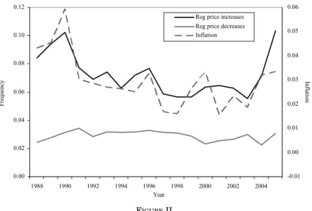
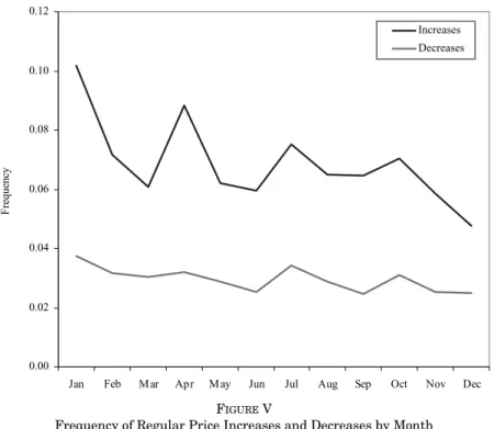
The second feature of price change that we investigate is the fraction of price changes that are price decreases. We find this fraction to be roughly one-third in both consumer prices excluding sales and finished-goods producer prices. We present a benchmark menu cost model along the lines of Golosov and Lucas (2007) and show that the fraction of price changes that are decreases helps pin down the key parameters of this model. The third feature of price change that we investigate is how the frequency and size of price change covaries with the inflation rate. We find that the frequency of price increases covaries quite strongly with the rate of inflation, whereas the frequency of price decreases and the size of price increases and decreases do not. This fact provides a natural test for our calibrated benchmark menu cost model. The fourth feature of price change that we investigate is the extent of seasonal synchronization. We find that price rigidity is highly seasonal both for consumer and producer prices. Prices are substantially more likely to change in the first quarter than in other quarters.
The fifth and final issue that we investigate is the haz-ard function of price change. The main empirical challenge in estimating the hazard function of price change is the fact that heterogeneity in the level of the hazard function across products—if not properly accounted for—leads to a downward bias in the slope of the hazard function. We use the empirical model of Meyer (1990) to account for heterogeneity. The hazard function of consumer prices including sales is steeply downward sloping for sectors with frequent sales. In contrast, the estimated hazard function of price change for both consumer prices exclud-ing sales and producer prices is slightly downward slopexclud-ing for the first few months and then mostly flat. The only substantial deviation from a flat hazard after the first few months is a large spike in the hazard at twelve months for services and producer prices.3We show that menu cost models can give rise to a wide calibrated to the mean duration of price spells in the economy replicates the de-gree of monetary nonneutrality in a multisector model. We present estimates of the mean duration in Table I.
3. Earlier empirical work on the hazard function of price changes includes Cecchetti (1986), Jonker, Folkertsma, and Blijenberg (2004), ´Alvarez, Burriel, and Hernando (2005), Baumgartner et al. (2005), Campbell and Eden (2005), Dias, Robalo Marques, and Santo Silva (2005), Foug´ere, Bihan, and Sevestre (2005), and Goette, Minsch, and Tyran (2005). Empirical support for upward-sloping hazard functions appears to arise mostly in studies in which almost all price changes are increases. Several of these papers use the conditional logit specification to account for unobserved heterogeneity. Unfortunately, this specification yields inconsistent estimates of the shape of the hazard function (Willis 2006).
variety of hazard functions, depending on the relative importance of inflation and idiosyncratic shocks. The hazard function implied by our calibrated benchmark menu cost model is sharply upward sloping for the first few months.
Klenow and Kryvtsov (2008) report related statistics regard-ing the frequency of price change, the relationship between the size and frequency of price adjustments and the ination rate, and the hazard function of price change. Their frequency of price change estimates are very similar to ours, although their interpretation of these statistics is somewhat different. They estimate the median implied duration of regular prices, including substitutions, to be 7.2 months. Their estimator is similar to the one we use in line 10 of Table I.4 A time-weighted average
of our estimates in line 10 of Table I is 7.5 months. For regular prices excluding substitutions, they report 8.7 months and a time-weighted average of our estimates is also 8.7 months (line 6 of Table I). They report a median implied duration of 9.3 months based on adjacent regular prices. A time-weighted average of our estimates is 9.6 months (line 3 of Table I). The range of numbers we report has a higher upper bound because we split the sample and report results separately for the subsample 1998–2005 for which the rate of inflation was lower.
An important body of work on price adjustment in Europe has been carried out by the Inflation Persistence Network of the European Central Bank. ´Alvarez et al. (2006) and Dhyne et al. (2006) summarize the conclusions of a number of papers on the frequency of price adjustment in consumer prices for the countries of the Euro area. Vermeulen et al. (2006) summarize analogous studies on producer prices in the Euro area. Fabiani et al. (2004) summarize survey evidence on price adjustment in the Euro area. Our findings regarding the frequency of price change, the relation-ship between the frequency of price increases and inflation, and the seasonality of price changes find strong support in a number of European countries.5
4. The main difference between the estimate in line 10 of Table I and the estimate used by Klenow and Kryvtsov (2008) is that their estimator does not condition on the state (regular price, sale, or stockout), whereas ours does.
5. A number of other recent papers have studied the frequency and size of price changes using disaggregated price data, including Lach and Tsiddon (1992), Baharad and Eden (2004), Konieczny and Skrzypacz (2005), Hobijn, Ravenna, and Tambalotti (2006), Midrigan (2006), Kackmeister (2007), and Gopinath and Rigobon (2008).
The paper is organized as follows. In Section II, we describe the data. In Section III, we present evidence on the frequency of price change, the fraction of price changes that are price in-creases, the frequency of product turnover, the absolute size of price changes, and temporary sales. In Section IV, we present and calibrate a benchmark menu cost model. In Section V, we present evidence on how the frequency and size of price changes vary with inflation. In Section VI, we present evidence on the seasonality of price changes and sales. In Section VII, we present our estimates of the hazard function of price change. Section VIII concludes.
II. THEDATA
We use two data sets gathered by the BLS in this paper. The first is the CPI Research Database. This is a confidential data set that contains product-level price data used to construct the CPI. The second is an analogous data set of producer prices that we have created from the production files underlying the PPI. We will refer to this data set as the PPI Research Database. The CPI Research Database has been used by Hosken and Reiffen (2007, 2004) and Klenow and Kryvtsov (2008).6The PPI Research
Database has not been used before.
II.A. The CPI Research Database
Each month the BLS collects prices of thousands of individual goods and services for the purpose of constructing the CPI. The CPI Research Database contains the nonshelter component of this data set from 1988 to the present. The goods and services included in the CPI Research Database constitute about 70% of consumer expenditures. Prices are sampled in 87 geographical areas across the United States. Prices of all items are collected monthly in the three most populous locations (New York, Los Angeles, and Chicago). Prices of food and energy are collected monthly in all other locations as well. Prices of other items are collected bimonthly. In most of our analysis, we use only monthly observations.7
6. Bils and Klenow (2004) used the BLS Commodities and Services Substitu-tion Rate Table for 1995–1997. The SubstituSubstitu-tion Rate Table contains the average frequency of price change including product substitutions and imputed missing values for all products in the CPI.
7. As a robustness test, we compared the bimonthly frequency of price change in the portion of our data set that is sampled bimonthly to the bimonthly fre-quency of price change in the portion of our data set that is sampled monthly. The
The CPI Research Database identifies products at an ex-tremely detailed level. In general, two products are considered different products in the database if they carry different bar codes. In addition, the same product at two different outlets is considered different products in the database. An example of a product in the database is a two-liter bottle of Diet Coke sold at a particular su-permarket in New York. The database reports whether a product was “on sale” when its price was sampled in a particular month.8
We use this sales flag to calculate statistics about the frequency and size of price change excluding sales. Some prices in the database are derived from the price of other products rather than being based on a collected price. We drop all such observations.9
The BLS divides products into so called Entry Level Items (ELIs). Examples of ELIs are “Carbonated Drinks,” “Washers & Driers,” “Woman’s Outerwear,” and “Funeral Expenses.” Before 1998, the BLS divided the data set into roughly 360 ELIs. In 1998, the BLS revised the ELI structure of the data set. Since then, it has divided the data set into roughly 270 ELIs. The revision in the ELI structure of the data set in 1998 implies that in many cases we calculate statistics separately for the periods 1988–1997 and 1998–2005. Most of our results are similar for the two sam-ple periods. For concreteness, we will refer to the estimates for the latter period in the text unless we indicate otherwise. In all of the statistics we present on the frequency and size of price changes, we focus on weighted medians and means across ELIs.
bimonthly frequency of price change is slightly lower in the bimonthly data than in the monthly data.
8. BLS field agents are instructed to mark a price as a sale price if it is considered by the outlet to be temporarily lower than the regular selling price and is available to all consumers. In practice, the BLS sales flag corresponds roughly to whether there is a “sale” sign next to the price when it is collected. If an outlet never sells a product at its “regular” price—that is, the product is always on sale— the BLS field agent is directed not to label it as a sale price. Sales available to customers with savings or discount cards are reported as sales only if the outlet confirms that more than 50% of its customers use these cards. Bonus items may be reported as sales as long as they satisfy the normal criteria for sales described above. Three categories in which the sale flag is never used by design are new and used cars and airfares. The approach that is used to collect price data for these categories is quite different from the procedure used to collect price data for other categories. The price series for new cars combines data on list prices with data on average “deals” obtained by consumers. The used car data are based on an index of used car prices. The data on airline tickets are based on a sample of tickets from the U.S. Department of Transportation data bank. Chapter 10 of the unpublished BLS manualPrice Reporting Rulescontains a more detailed description of the definition of sales used by the BLS.
9. Chapter 17 of theBLS Handbook of Methods(U.S. Department of Labor 1997) contains a far more detailed description of the consumer price data collected by the BLS.
The weights we use are CPI expenditure weights from 1990 for our statistics on the period 1988–1997 and weights from 2000 for our statistics on the period 1998–2005. The statistics at the ELI level are unweighted averages within the ELI.
II.B. The PPI Research Database
We construct the PPI Research Database from the production files underlying the U.S. PPI. The earliest prices in the database are from the late 1970s. For the period 1988–2005, which we focus on in most of our analysis, the PPI Research Database contains data for categories that constitute well in excess of 90% of the value weight for the Finished Goods PPI.10An important
difference between the CPI and the PPI is that the PPI is collected by BLS through a survey of firms. This methodology introduces greater concerns about data quality than in the CPI where BLS agents sample prices of products “on the shelf.” Stigler and Kindahl (1970) criticized the methodology used to gather the PPI data because it relied on “list” prices rather than transaction prices. Since then, the BLS has revamped its data collection methodology to focus expressly on collecting actual transaction prices. Specifically, the BLS requests the price of actual shipments transacted within a particular time frame.11 Note that many of
the transactions for which prices are collected as part of the PPI are part of implicit or explicit long-term contracts between firms and their suppliers. The presence of such long-term contracts makes interpreting PPI data more complicated than interpreting CPI data, as we discuss further in Section III.D.
Another difference between the consumer and producer price data is that the definition of a good in the PPI Research Database typically includes information about the buyer of the product as well as a detailed set of product and transaction characteristics. The definition is meant to capture all “price-determining vari-ables.” Price-determining variables may include the buyer, the quantity being bought, the method of shipment, the transaction terms, the day of the month on which the transaction takes place, and product characteristics. This implies that if a seller charges a different price to different customers, the BLS will collect prices for a transaction involving the same customer month after month.
10. The weights referred to here are the post-1997 value weights used to construct the Finished Goods PPI.
11. See Chapter 14 of theBLS Handbook of Methods(U.S. Department of Labor 1997) for a more detailed description of BLS procedures.
The price data in the PPI are collected in two steps. When a product is first introduced into the data set, the BLS collects “checklist” information by conducting a personal visit to the firm. The checklist contains information on characteristics of the prod-uct, buyer, and seller as well as the terms and date of the transac-tion. The checklist also contains information on various types of addendums to the standard price, for example, whether the price involves a trade or quantity discount or other type of discounts or surcharges. Once the product is initiated, price information is collected using a repricing form. The repricing forms are mailed or faxed. If the form is not returned, a BLS industry analyst calls the firm to collect information over the phone. The checklist in-formation is updated when an industry is resampled every five to seven years.
An important concern with the methods used to collect the PPI data is that the repricing form used to update prices in the PPI first asks whether the price has changed relative to the pre-vious month and then asks the respondent to report a new price if the price did change. This structure of the repricing form may introduce a bias toward no change into the data. To evaluate sen-sitivity of the price data to the method used to collect prices, we compared the behavior of prices during the anthrax scare of 2001 to the behavior of prices during other time periods. In October and November 2001, all mail to government agencies was rerouted, and PPI collected all prices by a phone survey. Controlling for the relationship between the frequency of price change and infla-tion, we found no significant differences in the frequency of price change in 2001 versus the same months in other years.12Another
feature of the data that suggests that the producer price data con-tain meaningful information is the high correlation between the frequency of price change for manufacturing prices and consumer prices excluding sales documented in Section III.E.
The BLS constructs indexes for three different stages of pro-cessing: finished goods, intermediate goods, and crude materials. We focus attention on finished goods, but also report basic results
12. The idea of using the anthrax scare of 2001 for this purpose is due to Gopinath and Rigobon (2008). Our approach is slightly different than theirs. We compare the frequency of price change during the anthrax scare with the frequency of price change in the same months of other years rather than the adjacent months because the frequency of producer prices is highly seasonal. Specifically, we regress the absolute size and frequency of price change in October and November of each year on a dummy for 1998 and the PPI. The coefficient on the “anthrax dummy” in the frequency regression is 0.0057 with a standard error of 0.0084, and in the absolute size regression it is 0.0041 with a standard error of 0.0030. Neither coefficient is statistically significant.
for intermediate goods and crude materials. Our method for cal-culating statistics at various levels of aggregation in the PPI is somewhat more complicated than in the CPI. The most detailed grouping in the PPI Research Database is the cell code. We do not attempt to construct value weights at this level because there is a substantial amount of churning in the cell codes used in the PPI from year to year. We instead obtain value weights for the PPI at the four-digit commodity code level. We then construct statis-tics on the frequency of price change at the four-digit commodity code level in the following way. First, we calculate the unweighted average frequency of price change within cell codes. Next, we cal-culate the unweighted median frequency of price change across cell codes within the four-digit commodity code. Finally, we con-struct aggregate statistics by taking value-weighted medians over the median price change frequencies at the four-digit commod-ity code level. This approach is similar to the approach taken by Gopinath and Rigobon (2008) for import and export price data. For the purpose of matching PPI categories with CPI ELIs, we con-struct unweighted medians within six-digit and eight-digit prod-uct categories.
III. HOWOFTEN ANDHOWMUCHDOPRICESCHANGE?
In this section, we present statistics on the frequency and size of price changes in the U.S. economy. While this may seem straightforward, there are a number of important issues to be con-sidered. We therefore discuss the construction of these statistics in some detail. An important lesson from the theoretical litera-ture on price adjustment is that different types of price adjust-ments have substantially different macroeconomic implications. The menu cost model has the strong prediction that the products “selected” to change their prices in response to an expansionary monetary shock disproportionately have prices that are far below their current optimum level. As a consequence of this selection effect, the price level responds relatively rapidly to the shock, and the effects of the shock on aggregate output are relatively transient (Caplin and Spulber 1987; Golosov and Lucas 2007). In contrast, if the timing of price changes is random, as in the Calvo (1983) model, monetary shocks have significantly more persistent effects on output.
Motivated by this theoretical literature, we distinguish between three broad classes of price changes: (1) regular price changes for identical items, (2) temporary sales, and (3) price
changes due to product substitution. We present statistics for these different types of price changes separately. We document that sales have empirical characteristics very different from regular price changes. Price changes associated with sales are highly transient and the price of the product returns to the old regular price after most sales. Kehoe and Midrigan (2007) argue that transitory price changes, such as temporary sales, yield much less aggregate price flexibility than an equal number of permanent price changes.
Our motive for distinguishing between price changes asso-ciated with product substitution and price changes for identical items is that new product introduction is motivated by many factors other than a firm’s desire to change its price. Product substitutions are by far most common in the apparel and transportation sectors. In these sectors, the introduction of new products is driven by factors such as the fall and spring clothing seasons, and the new model year for automobiles. Although the introduction of the new spring clothing line may be a good opportunity for a firm to adjust its price, this type of new product introduction does not occurbecauseof the firm’s desire to adjust its price, limiting the strength of the selection effect.
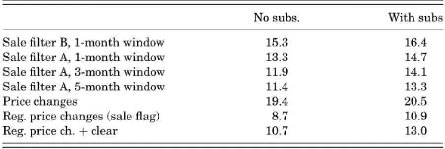
Two important measurement issues arise. First, how do we identify the presence of temporary sales? The BLS gathers data on whether a product was “on sale” when its price was sampled in a particular month. We use this sale flag as our primary measure of the presence of temporary sales.13We also consider identifying
sales based on a “sale filter” in Section III.H. Second, estimating the frequency of adjustment for regular prices is complicated by times when firms’ regular prices are not observed because of sales and stockouts. In the absence of a theory of sales and stockouts, there is no unique way of filling in these gaps in the regular price series.14 We present four estimates of the frequency of regular
13. This is the approach adopted by Bils and Klenow (2004) and the main approach used by Klenow and Kryvtsov (2008).
14. One can object to the notion that it is meaningful to say that a latent regular price exists during sales and stockouts. After all, the good is not available at the regular price in the case of sales and not available at all in the case of stockouts. However, the fact that the regular price of the product is often the same after sales and stockouts as before suggests that the old regular price should be viewed as a latent state variable in the firm’s pricing problem. Also, anecdotial evidence suggests that many sales take the form of a discount relative to the product’s most recent regular price, suggesting that the latent regular price influences the sale price. Finally, high-frequency data suggest that most sales and stockouts last for a much shorter period than an entire month. This implies that the products may
A
B
R R R R . R R S R R
No sales: 0 1 0 . . 0 . . 0
With sales: . .
0 1 0 . . 0 1 1 0
R R R R . R R S R R
No sales: . 0 1 0 . . 0 . . 0
With sales: . 0 1 0 . . 0 1 1 0
FIGUREI
Construction of Price Change Variables with and without Sales
Notes. Each panel reports the first ten observations for a hypothetical price series. The top row of each panel records the values of the sales flag for the ten observations. The letter “R” denotes “regular price” while the letter “S” denotes “sales.” Below the flag is a graph of the evolution of the price of the product. At the bottom of each panel are two indicator variables. The first records price changes, while the second records regular price changes.
price change corresponding to four different treatments of regular prices during sales and stockouts.
The simplest approach is to estimate the frequency of regular price change during periods when the presence or absence of reg-ular price changes is directly observable, that is, when contiguous nonsale observations are made. Figure I graphically illustrates this simple procedure. The two panels in the figure report the first ten observations for two hypothetical products. Each panel con-tains a graph of the evolution of the price of the product for these ten observations. At the top of each panel in the figure, we record with the letter “R” and the letter “S” whether each observation is a regular price or a sale, respectively. At the bottom of each panel,
in fact be available at some unobserved regular price for a large fraction of the month in question.
there are indicator variables that record price changes including and excluding sales. First, notice that the price change variable is missing for the first observation. This is because the price in the previous month is not observed. Second, notice that the fifth price observation is missing. This yields two missing values in the price change variable. Third, notice that the eighth observation is a sale. The sale yields two price changes in the “raw” price change variable. However, dropping the sale observation from the data set yields two missing observations for the regular price change variable. In this example, our estimate of the frequency of regular price change based on contiguous observations would therefore be 1/5=20%.
This procedure has the advantage that it does not make any assumption regarding the behavior of the unobserved regular price series over the course of the sale. It provides a direct estimate of the extent of price flexibility that does not arise from sales. Yet, this procedure has the disadvantage that it does not incorporate in any way information in the data set about whether a product’s regular price is the same before and after sales and stockouts. If regular prices follow a constant hazard model, then the frequency of regular price change during the periods when regular prices are observed provides a good estimate of the frequency of regular price change during periods when regular prices are not observed.15
However, the behavior of regular prices may be systematically different over the course of sales and stockouts than during other periods. In this case, the implied durations of regular prices asso-ciated with this method are likely to be systematically biased.
Our second procedure for calculating the frequency of price change assumes that the latent regular price series is equal to the last observed regular price until a change is observed. This is the procedure used by Klenow and Kryvtsov (2005) and Gopinath and Rigobon (2008). In the context of the menu cost model, this procedure would be appropriate if regular prices were systemati-cally readjusted at the end of (but not during) sales or stockouts. To implement this procedure, we carry forward the last observed regular price through sale and stockout periods and calculate the
15. It may at first seem that the procedure based only on contiguous observa-tions necessarily underestimates the frequency of regular price change because it does not count regular price changes during sales and stockouts. In this regard, it is important to notice that while using only contiguous observations leads one to drop a price change during the sale in Panel B, it also causes one to drop a “no change” during the sale in period A and during the stockout in both panels. If the probability of regular price change is the same during sales and stockouts as it is during other periods (as in a constant hazard model) then dropping the sale price observations has no systematic effect on the estimates.
frequency of price change of the resulting series.16This procedure has the appealing feature that it captures the price changes and “no changes” after sales and stockouts in a particularly simple way. However, it assumes that only one regular price change can occur over the course of a sale or stockout. It therefore assumes a maximum amount of rigidity during sales and stockouts.
Our third procedure makes the assumption that the latent regular price series evolves stochastically over the course of a sale. In the context of the menu cost model, this procedure would be appropriate if regular prices were adjusted both during and after sales. The key difference between this procedure and the previous ones is that it allows for more than one price change over the course of the period when regular prices are unobserved. To implement this procedure, we take the following weighted average: (1−s)f+s f, where f is the measure of the frequency of price change based on contiguous nonsale, nonstockout obser-vation, f is a direct estimate of the frequency of regular price change during one- and two-month sales, andsis the fraction of price change observations corresponding to sales.17 Our fourth
procedure is analogous to the third procedure except that it estimates a separate process for latent regular prices during both sales and stockouts. This is a very similar procedure to the one used by Klenow and Kryvtsov (2008).
16. We carry forward prices if they are followed by another regular price within five months. For longer gaps, we do not fill in the missing observations. It is not obvious how to construct statistics on price flexibility for goods that are not always available. Analogous to stockouts, almost all stores close at night. One could therefore say that prices all rise to infinity at night as well as during stockouts. Consider one economy with 24-hour stores and another with 12-hour stores that both reset all prices on January 1. One measure of price flexibility would be the frequency of price change relative to the total amount of time the good is available. According to this measure the second economy has twice as much price flexibility as the first. Yet prices in the latter economy would not respond more rapidly to aggregate shocks. In contrast, suppose all goods in the economy are available for only one month a year and firms reset their prices at that time. In this economy, prices are perfectly flexible even though the price of each good changes only once a year. The key distinction is whether prices reflect current economic conditions. This distinction motivates our decision to carry prices forward only for four months or less.
17. We calculate f=ω1f1+(1−ω1)f2, where f1and f2are the monthly fre-quency of regular price change during one- and two-periods sales, respectively. These frequencies are estimated using the method described in Section III.B.;ω1 is the fraction of sales that are one-period sales. In small samples, this proce-dure yields an upward-biased estimate of the probability of price change during sale and missing periods due to Jensen’s inequality. We have considered other weighted averages of sales spells of different lengths; this choice makes little dif-ference because most sales spells are short. We only make use of cases where a price is observed before and after the event in calculating the probability of price change over the course of sales and stockouts. In particular, clearance sales do not contribute to these statistics.
Following Bils and Klenow (2004) and Dhyne et al. (2006), we have focused on estimating the frequency of price change. An alternative empirical strategy is to record the duration of each price spell and calculate the weighted median duration across all price spells. However, the presence of a large number of censored price spells complicates this approach. To account for right cen-soring, one must estimate a hazard model. This is a challenging problem because of the presence of heterogeneity. Left censoring is particularly problematic in applications with heterogeneity. The standard practice in the duration literature is to drop left-censored spells. This introduces an initial-conditions problem that biases the estimated duration downward in the presence of heterogene-ity (Heckman and Singer 1986). Intuitively, longer spells are more likely to be left censored.
III.A. The Frequency of Price Change: Consumer Prices
Table I reports estimates of the frequency of price change for nonshelter goods and services in the CPI. The first two columns in the table report estimates for the median frequency of price change excluding and including both sales and substitutions.18
Our four estimates of the median frequency of regular price change for identical items range from 8.7% per month to 11.9%, depending on the sample period and treatment of missing obser-vations. We define the corresponding median implied duration to bed= −1/ln(1− f), where f is the median frequency.19 These
estimates therefore imply median durations of eight to eleven months. Procedures 3 and 4 yield higher estimates than Proce-dure 1 because the frequency of regular price change over the course of sales and stockouts is estimated to be on average about 2 percentage points higher than during other periods. Including substitutions raises the frequency of price change by 1–2 percent-age points (Panel C).20
18. These statistics are estimated by first calculating the mean frequency of price change for each ELI and then taking a weighted median across ELIs.
19. A constant hazardλof price change implies a monthly probability of a price change equal tof=1−e−λ. This impliesλ= −ln(1− f) andd=1/λ= −1/ln(1−
f). In the case of statistics where substitutions are excluded, the implied duration is an estimate of duration where product exit is viewed as a censoring event. In other words, it is a measure of the median uncensored duration.
20. Our procedure in row (10) of Table I is similar to the procedure used by Klenow and Kryvtsov (2008). The main difference is that our procedure allows for a different frequency of price change during sales/stockout than during periods when the regular price is observed.
T ABLE I F REQUENCY O F P RICE C HANGE IN T HE CPI Median frequency M edian implied d uration M ean frequency Mean implied d uration 1988–1997 1998–2005 1988–1997 1998–2005 1988–1997 1998–2005 1988–1997 1998–2005 (%) (%) (months) (months) (%) (%) (months) (months) A. Inc luding sales Exc luding substitutions 20.3 19.4 4 .4 4.6 23.9 26.5 8 .3 9.0 Inc luding substitutions 21.7 20.5 4 .1 4.4 25.2 27.7 7 .5 7.7 B . Exc luding sales and substitutions Contiguous observations 11.1 8 .7 8.5 11.0 18.7 21.1 11.6 13.0 Carry regular p rice forw ard d uring sales a nd stoc kouts 11.2 9 .0 8.4 10.6 18.6 20.9 11.0 12.3 Estimate frequency o f p rice ch ange during sales 11.5 9 .6 8.2 9 .9 19.0 21.3 11.2 12.5 Estimate frequency o f p rice ch ange during sales a nd stoc kouts 11.9 9 .9 7.9 9 .6 18.9 21.5 10.8 11.7 C . Exc luding sales , inc luding substitutions Contiguous observations 12.7 10.9 7 .4 8.7 20.4 22.8 9 .3 9.8 Carry regular p rice forw ard d uring sales a nd stoc kouts 12.3 10.6 7 .6 8.9 19.7 22.0 9 .6 10.4 Estimate frequency o f p rice ch ange during sales 12.8 11.3 7 .3 8.3 20.8 22.8 9 .2 9.8 Estimate frequency o f p rice ch ange during sales a nd stoc kouts 13.0 11.8 7 .2 8.0 20.7 23.1 9 .0 9.3 Notes . All frequencies are reported in p ercent per m onth. Implied d urations are reported in m onths . “Median frequency” d enotes the w eighted m edian frequen cy of price change . It is calculated by first calculating the mean frequency o f p rice ch ange for e ac h E LI and then taking a weighted median across ELIs within the m ajor group using C PI expenditure weights . The “Median implied d uration” is equal to − 1 / ln(1 − f ), where f is the m edian frequency of price change . “Mean frequency” d enotes the w eighted m ean frequency of price ch ange . “Mean implied d uration” denotes the weighted implied d uration o f p rice ch ange . It is calculated b y fi rst calculating the implied d uration for eac h ELI a s − 1 / ln(1 − f ), where f is the frequency of price change for a particular E LI, a nd then taking a w eighted m ean a cross E LI’ s using C PI expenditure w eights .
In contrast, the frequency of price change for identical items including sales was 19.4% for 1998–2005 and 20.3% for 1988– 1997, implying median durations of 4.6 months and 4.4 months, respectively. The frequency of regular price change is therefore roughly 50% lower than the frequency of price change including sales. Adjusting for sales makes such a large difference not only because sales are common in the data—the expenditure-weighted fraction of price changes due to sales is 21.5%—but also because of the uneven distribution of sales across goods. Table II reports the fraction of price change due to sales by major group. On the one extreme, 87.1% of price changes in apparel and 66.8% of price changes in household furnishings are due to sales. On the other, virtually no price changes in utilities, vehicle fuel, and services—a category that has an expenditure weight of 38.5%—are due to sales.
The sectors that have few sales tend to have either very high (utilities, vehicle fuel and travel) or very low (services) unadjusted frequencies of price change. The sales adjustment is therefore concentrated in sectors that start off with a frequency of price change that is relatively close to the median frequency of price change. This heterogeneity in the prevalence of sales implies that the median frequency of price change drops by roughly 50% when sales are excluded, rather than 21.5%.21
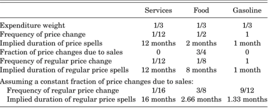
To see this point more clearly, consider the three-sector ex-ample presented in Table III. Suppose the three sectors in the economy are services, food, and gasoline. Each has an expendi-ture weight of 1/3. Prices of services change once a year and have no sales. Prices of food change every other month, but 3/4 of these price changes are sales. The price of gasoline changes every month and gasoline never goes on sale. In this example, as in our data, sales are concentrated in the sector that is in the middle of the distribution of price change frequency. Adjusting for sales sec-tor by secsec-tor yields a median frequency of regular price change of 1/8 and a median duration of 8 months. However, applying a blanket adjustment of 3/12 to all sectors—the overall fraction of
21. Bils and Klenow (2004) also present a statistic on the frequency of price change adjusted for sales. Because of data limitations, they were not able to adjust for sales at the good level. Instead, they adjusted the median frequency of price change by the fraction of price changes due to sales in the entire data set. This procedure yields an estimate of the sales-adjusted median duration of 5.5 months. It is a valid adjustment for sales under the assumption that sales account for the same fraction of price changes in all sectors. As we discuss, this assumption is dramatically at odds with the data.
T ABLE II F REQUENCY O F P RICE C HANGE B Y M AJOR G ROUP IN 1998–2005 Regular p rices P rices S ales Median Median Mean Mean F rac . F rac . Major g roup W e ight F req. Impl. dur . freq. F rac . up F req. Impl. dur . freq. F rac . up price ch. obs . Processed food 8 . 21 0 . 59 . 01 0 . 66 5 . 42 5 . 93 . 32 5 . 55 4 . 75 7 . 91 6 . 6 Unprocessed food 5 . 92 5 . 03 . 52 5 . 46 1 . 23 7 . 32 . 13 9 . 55 3 . 33 7 . 91 7 . 1 Household furnishing 5 . 06 . 01 6 . 16 . 56 2 . 91 9 . 44 . 62 0 . 64 9 . 06 6 . 82 1 . 2 Apparel 6 . 53 . 62 7 . 33 . 65 7 . 13 1 . 02 . 73 0 . 13 6 . 18 7 . 13 4 . 5 Transportation goods 8 . 33 1 . 32 . 72 1 . 34 5 . 93 1 . 32 . 72 2 . 24 4 . 08 . 02 . 7 Recreation g oods 3 . 66 . 01 6 . 36 . 16 2 . 01 1 . 97 . 91 3 . 75 1 . 34 9 . 11 0 . 9 Other g oods 5 . 41 5 . 06 . 11 3 . 97 3 . 71 5 . 55 . 92 0 . 66 1 . 33 2 . 61 5 . 3 Utilities 5 . 33 8 . 12 . 14 9 . 45 3 . 13 8 . 12 . 14 9 . 45 3 . 10 . 00 . 0 V e hic le fuel 5 . 18 7 . 60 . 58 7 . 45 3 . 58 7 . 60 . 58 7 . 55 3 . 40 . 00 . 3 Tra v el 5 . 54 1 . 71 . 94 3 . 75 2 . 84 2 . 81 . 84 4 . 45 2 . 21 . 52 . 1 Services (exc l. tra v el) 3 8 . 56 . 11 5 . 88 . 87 9 . 06 . 61 4 . 69 . 17 6 . 83 . 10 . 5 All sectors 100 . 08 . 71 1 . 02 1 . 16 4 . 81 9 . 44 . 62 6 . 55 7 . 12 1 . 57 . 4 Notes . All frequencies are reported in p ercent per m onth. D urations are reported in m onths . F ractions a re reported as percentages . Regular p rices d enote p rices exc luding sales . “W eight” denotes the CPI e xpenditure weight of the m ajor group; “median freq. ” d enotes the w eighted m edian frequency of price change . It is calculate db yfi rs tc a lc u la ti n g th em e a n frequency o f p rice ch ange for e ac h E LI and then taking a weighted median across ELIs within the m ajor group u sing CPI e xpenditure weights . The o ther med ian statistics in this table a re calculated in an analogous m anner: “median impl. dur .” is e qual to − 1 / ln(1 − f ), where f is the m edian frequency of price change . “Mean freq. ” d enotes the e xpenditure weighted mean frequency o f p rice ch ange; “frac . u p” denotes the median fraction of price changes that are p rice increases; “frac . p rice ch .” and “frac . o bs .” denote the e xpenditure weighted mean fraction of price changes that are d ue to sales a nd fraction of observations that are sales . T he sector weights add up to 97.4% because u se d cars a re not inc luded in any sector .
TABLE III
SALESADJUSTMENTWHENSALESARECONCENTRATED INCERTAINSECTORS
Services Food Gasoline
Expenditure weight 1/3 1/3 1/3
Frequency of price change 1/12 1/2 1
Implied duration of price spells 12 months 2 months 1 month
Fraction of price changes due to sales 0 3/4 0
Frequency of regular price change 1/12 1/8 1
Implied duration of regular price spells 12 months 8 months 1 month Assuming a constant fraction of price changes due to sales:
Frequency of regular price change 1/16 3/8 9/12
Implied duration of regular price spells 16 months 2.66 months 1.33 months
Notes.In this example the expenditure-weighted fraction of price changes due to sales is 3/12. Assuming
that the fraction of price changes due to sales is the same across sectors, the frequency of regular price change equals the frequency of price change multiplied by 1−3/12=9/12. For simplicity, we assume that only one price change can occur per month in this example.
price changes due to sales in the entire economy—yields a me-dian frequency of price change of 3/8 and a meme-dian duration of 2.67 months.
There is a huge amount of heterogeneity in the frequency of regular price change across sectors in the U.S. economy (Table II). Furthermore, the distribution of the frequency of regular price change is very right skewed. Most of the mass of the distribution lies below a frequency of regular price change of 12%, whereas cat-egories such as vehicle fuel have a frequency of price change sub-stantially higher than 50%. As a consequence, the mean frequency of regular price change is almost twice the median frequency of regular price change. Table I reports that the weighted mean frequency of price change in the 1998–2005 period is 26%–28% including sales and 21%–22% excluding sales. These estimates are consistent with the estimates of Klenow and Kryvtsov (2005). Table I also reports the weighted mean implied durations for the various alternative procedures for calculating the frequency of price change. Jensen’s inequality implies that the mean implied duration is not the same as the implied duration for a product with the mean frequency of price change. Our estimates of the mean implied duration lie between 9 and 13 months.
One issue that arises in considering the macroeconomic im-plications of sales is that the quantity sold on sale is likely to be disproportionately large relative to the fraction of time the product is on sale. In the extreme, suppose all of the volume for a particular
product is sold on sale. In this case, does the rigidity of the regular price influence real quantities? The answer to this question de-pends on whether sale prices are set entirely independently from nonsale prices or sale prices are partially set relative to a prod-uct’s regular price (e.g., 20% discount). In the second case, even if all products are sold on sale, the rigidity of regular prices still influences real quantities through its effect on the sales prices.
III.B. Behavior of Prices after Sales
Sales exhibit empirical features markedly different from reg-ular price changes.22Table IV presents statistics on sales for the
four major groups for which sales are most important: processed food, unprocessed food, household furnishings, and apparel. First, sales are much shorter than regular price spells. The fraction of sales that last just one period ranges between 35% and 60% in the four major groups in Table IV, and the average length of sales is just 1.8–2.3 months. Longer sales are more prevalent in apparel and household furnishings because clearance sales tend to be longer than other sales and are relatively frequent in these sectors.
Second, the price of a product usually returns to its original regular price following a sale. For the major groups in Table IV, prices return to their original regular price between 60.0% and 86.3% of the time after a one-period sale. Evidently, many sales price changes are highly transient. Clearance sales are not in-cluded in these statistics because a new regular price is not observed after the sale. Yet, clearance sales, like other types of sales, yield highly transient price changes, as we discuss in the supplementary material to this paper.23
22. Explanations for sales in the industrial organization literature may be grouped into two categories: (1) intertemporal price discrimination (Varian 1980; Sobel 1984) and (2) inventory management (Lazear 1986; Pashigian 1988; Aguirregabiria 1999). Hosken and Reiffen (2004) use CPI data to evaluate the empirical implications of these models.
23. Our evidence regarding the length of sales and the fraction of price changes that return to the original regular price is limited by the fact that our data set samples prices only once a month. Higher frequency data sets suggest that many sales are substantially shorter than one month (Pesendorfer 2002). This suggests that our estimates of the length of sales are upward biased and that our estimates of the fraction of price changes that return to the original price are downward biased. The fractions reported in Table IV imply that the frequency of regular price change during sales is highly correlated with the frequency of regu-lar price change during nonsale periods and only slightly higher on average. The supplementary material is available both on the QJE website and the personal websites of the authors.
T ABLE IV S ALES AND P RICES D URING S ALES F req. p rice ch . F rac . return F rac . o f sales F req. p rice ch . F req. reg . d uring o ne-period a fter one-period that last during one-period A v. d ur . price ch. sales sales one p eriod sales/miss . sales Processed food 10.5 11.4 78.5 64.7 11.1 2 .0 Unprocessed food 25.0 22.5 60.0 63.2 22.1 1 .8 Household furnishings 6.0 11.6 78.2 43.3 9 .4 2.3 Apparel 3.6 7 .1 86.3 35.8 5 .9 2.1 Notes . The sample p eriod is 1998–2005. “F req. reg . price ch. ” d enotes the m edian frequency of price changes exc luding sales . “F req. p rice ch . d uring o ne-per iod sales” d enotes the m edian m onthly frequency o f regular price change d uring sales that last one m onth. T he monthly frequency is calculated as 1 − (1 − f ) 0 . 5 where f is the fraction o f p rices that return to their o riginal level after o ne-period sales . “F rac . return a fter one-period sales” denotes the median fraction of prices that return to the ir original level a fter one-period sales . “F rac . of sales that last o ne period” d enotes the m edian fraction o f sales that last one m onth. In calculating this statistic w e d rop left-censored sal e spells . M edians are calculated b y first calculating a n a verage within eac h ELI a nd then calculating a n e xpenditure-weighted m edian a cross E LIs w ithin the major g roup . “F req. p rice ch . during one-period sales/miss .” denotes the median monthly frequency of regular p rice ch ange during sales o r m issing periods that last o ne month, calculated in the m anner d escribed a bove for sales . “A v. d ur . sales” denotes the weighted a v erage d uration o f sale p eriods in months .
TABLE V
FREQUENCY OFSUBSTITUTION ANDPRICECHANGE BYCATEGORY Pr. ch. w/subs Price change Subs.
Major group Weight freq. Freq. reg. Freq. Freq. reg. Freq.
Processed food 8.2 1.3 10.9 26.1 10.5 25.9
Unprocessed food 5.9 1.2 25.6 37.2 25.0 37.3
Household furnishing 5.0 5.0 9.2 20.6 6.0 19.4
Apparel 6.5 9.9 7.9 32.2 3.6 31.0
Transportation goods 8.3 10.2 36.6 36.6 31.3 31.3
Recreation goods 3.6 6.3 7.3 14.3 6.0 11.9
Other goods 5.4 1.0 15.4 16.2 15.0 15.5
Utilities 5.3 0.6 38.5 38.5 38.1 38.1
Vehicle fuel 5.1 0.2 87.6 87.6 87.6 87.6
Travel 5.5 1.9 42.5 43.5 41.7 42.8
Services (excl. travel) 38.5 0.9 7.2 7.4 6.1 6.6
Notes.The sample period is 1998–2005. “Subs. freq.” gives the median monthly frequency of price changes
associated with forced item substitutions in the Consumer Price Index as a fraction of all months in which the product is available, as well as intermediate periods of five months or less when the product is unavailable at the time of sampling but subsequently becomes available. Pr. ch. w/subs denotes the median monthly frequency of price change including price changes due to product substitutes. “Price change” indicates the median monthly frequency of price change. The median statistics are calculated by first calculating the mean frequency of price change or substitutions within ELIs and then calculating the expenditure-weighted median across ELIs. “Weight” denotes the expenditure weight of the ELI. The sector weights add up to 97.4% because used cars are not included in any sector.
In the sections that follow, we document three additional char-acteristics of sales that differ from regular price changes: (1) sale price changes are more than twice as large as other price changes on average; (2) sales have a very different relationship to aggre-gate variables such as inflation than regular price changes; and (3) the hazard function of price change including sales is much more downward sloping than the hazard function of price change for regular prices.
III.C. Product Substitutions
The literature on price rigidity has focused primarily on mod-eling and measuring the frequency of price change for identical items. However, in many durable goods sectors of the economy, the primary mode of price adjustment is not price changes for identical items; it is product turnover. Table V reports information on product substitutions for consumer products. Because product introductions involve pricing decisions, the frequency of product introduction would be the ideal measure of product turnover for the purpose of measuring price flexibility. The CPI Research Database provides an imperfect measure of product introduction
by providing an indicator for whether a product undergoes a “forced substitution.” A forced substitution occurs if the BLS is forced to stop sampling a product because it becomes permanently unavailable.24
The main complication that arises in relating the frequency of substitutions to the frequency of product introduction is that our data set does not follow products over their entire lifetime. Following a substitution, the BLS procedure for choosing a new product to sample tends to lead to the selection of products that have existed for some time.25If older products are more likely to
become permanently unavailable than new ones, then the average frequency of forced product substitution is an upward-biased mea-sure of the average frequency of product introduction. Despite this caveat, the frequency of substitutions provides useful information on the frequency of product turnover. We measure the frequency of substitutions as a fraction of the total product lifetime.26
Substitutions are most common in durable goods categories, particularly apparel and transportation goods. In apparel, we es-timate the frequency of substitutions to be 9.9%. Many clothes categories undergo substitutions twice a year at the beginning of the spring and fall seasons. For some clothes, such as women’s dresses, substitutions are even more common. Substitutions are also common in transportation goods. In this category, the monthly rate of substitutions is 10.2%. This high rate of substitutions is driven by the introduction of the new model year in cars each fall. Household furnishings and recreation goods also have high rates of substitution, 5.0% and 6.3%, respectively. Other product categories have a rate of substitutions close to 1%.27
24. Moulton and Moses (1997) show that price changes that are concurrent with product substitutions play a disproportionate role in explaining steady-state aggregate inflation. This effect is particularly strong in apparel where “clearance sales” are common just before product substitutions.
25. When a product in the data set becomes unavailable, BLS pricing agents are instructed to substitute the most similar available product. In sectors where fashion is important, this is likely to be an older product.
26. We define a product’s lifetime as the total time the product is priced and available, where we also include periods when the product is temporarily unavail-able for five months or less. This definition is meant to capture the idea that permanent product exits are likely to be followed by new product introductions; but a new product introduction is less likely to occur when the product is only tem-porarily absent. This measure differs from the measure used by Bils and Klenow (2004). They define the frequency of substitutions as a fraction of the total number of prices collected. We exclude product substitutions that do not lead to a price change because these substitutions do not yield additional price flexibility.
27. See the supplementary material to this paper for a detailed analysis of the timing and frequency of product substitutions in different sectors of the U.S. economy.
In categories such as apparel and transportation goods, the timing of product substitution is primarily motivated by factors such as seasonal demand variation, fashion, and product cycles rather than a firm’s desire to change its price. Price changes oc-cur when new products are introduced. But new products are not introduced because the old products were mispriced. This implies that the selection effect associated with price changes due to prod-uct substitution may be weaker than for price changes for identical items (Nakamura and Steinsson 2007). The degree of aggregate price flexibility induced by price changes due to product substitu-tion is therefore likely to be less than that induced by the same number of price changes for identical items.
III.D. Frequency of Price Change: Producer Prices
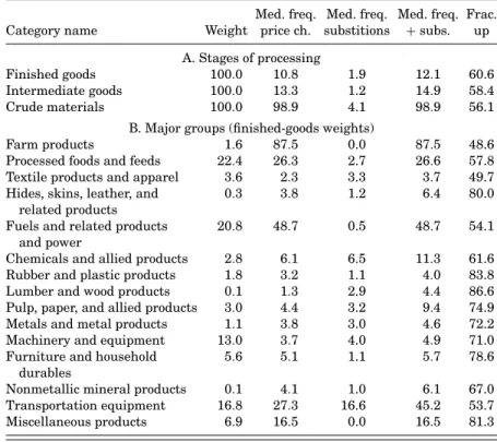
Panel A of Table VI presents statistics on the median fre-quency of price change for producer prices at three different stages of processing: finished goods, intermediate goods, and crude ma-terials. The median frequency of price change of finished producer goods in 1998–2005 was 10.8%. The corresponding median implied duration is 8.7 months. The median frequency of price change of intermediate goods in 1998–2005 was 13.3%, and the correspond-ing median implied duration is 7.0 months. In contrast to finished goods and intermediate goods, crude materials have almost com-pletely flexible prices. The median frequency of price change of crude materials in 1998–2005 was 98.9%, and the corresponding median implied duration is 0.2 months. Sales do not appear to be common in our producer price data set.28 We therefore make no adjustment for sales when analyzing producer prices.
In the PPI, a relatively small (value-weighted) fraction of the categories have a frequency of price change close to the median. Most of the categories with frequencies of price change above the median, have frequencies of price change substantially higher than 10%. As a consequence, the 55th percentile is 18.7% for 1998– 2005, while the median is 10.8%. In contrast, for the CPI the 55th percentile is 10.1% for 1998–2005, while the median is 8.7%.
Panel B of Table VI reports results on the frequency of price change of producer prices by two-digit major groups. As in the case of consumer prices, there is a large amount of heterogeneity
28. The PPI database does not include a sales flag. We used the sales filters described in Section III.H to assess the importance of sales in the producer price data. These sales filters identified very few sales.
TABLE VI
FREQUENCY OFPRICECHANGE FORPRODUCERPRICES
Med. freq. Med. freq. Med. freq. Frac.
Category name Weight price ch. substitions +subs. up
A. Stages of processing
Finished goods 100.0 10.8 1.9 12.1 60.6
Intermediate goods 100.0 13.3 1.2 14.9 58.4
Crude materials 100.0 98.9 4.1 98.9 56.1
B. Major groups (finished-goods weights)
Farm products 1.6 87.5 0.0 87.5 48.6
Processed foods and feeds 22.4 26.3 2.7 26.6 57.8
Textile products and apparel 3.6 2.3 3.3 3.7 49.7
Hides, skins, leather, and 0.3 3.8 1.2 6.4 80.0
related products
Fuels and related products 20.8 48.7 0.5 48.7 54.1
and power
Chemicals and allied products 2.8 6.1 6.5 11.3 61.6
Rubber and plastic products 1.8 3.2 1.1 4.0 83.8
Lumber and wood products 0.1 1.3 2.9 4.4 86.6
Pulp, paper, and allied products 3.0 4.4 3.2 9.4 74.9
Metals and metal products 1.1 3.8 3.0 4.6 72.2
Machinery and equipment 13.0 3.7 4.0 4.9 71.0
Furniture and household 5.6 5.1 1.1 5.7 78.6
durables
Nonmetallic mineral products 0.1 4.1 1.0 6.1 67.0
Transportation equipment 16.8 27.3 16.6 45.2 53.7
Miscellaneous products 6.9 16.5 0.0 16.5 81.3
Notes.The sample period is 1998–2005. Frequencies are reported in percent per month. Fractions are
reported in percentages. “Weight” denotes the post-1997 final goods value weight of the major groups. “Med. freq. price ch.” denotes the median frequency of price change. It is calculated by first calculating the mean frequency of price change for each cell code, then taking an unweighted median within the four-digit commodity code, and then taking a value-weighted median across four-digit commodity codes. “Frac. up” denotes the median fraction of price increases. It is calculated in a manner analogous to the median frequency of price change.
across sectors. Table VI also reports the frequency of product substitution for these two-digit major groups. The frequency of product substitution varies across the major groups from 0% in farm products to 16.6% in transportation goods.
The finding that finished-goods producer prices exhibit a sub-stantial degree of rigidity confirms for a broader set of products the results of a number of previous studies (e.g., Blinder et al. [1998]; Carlton [1986]). Interpreting this evidence is, however, more com-plicated than interpreting evidence on consumer prices. Buyers and sellers often enter into long-term relationships in wholesale markets. It is therefore possible that buyers and sellers enter
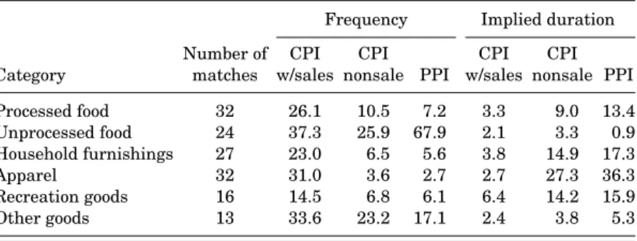
TABLE VII
FREQUENCY OFPRICECHANGE: COMPARISON OFCPIANDPPI CATEGORIES
Frequency Implied duration
Number of CPI CPI CPI CPI
Category matches w/sales nonsale PPI w/sales nonsale PPI
Processed food 32 26.1 10.5 7.2 3.3 9.0 13.4
Unprocessed food 24 37.3 25.9 67.9 2.1 3.3 0.9
Household furnishings 27 23.0 6.5 5.6 3.8 14.9 17.3
Apparel 32 31.0 3.6 2.7 2.7 27.3 36.3
Recreation goods 16 14.5 6.8 6.1 6.4 14.2 15.9
Other goods 13 33.6 23.2 17.1 2.4 3.8 5.3
Notes.“Number of matches” denotes the number of ELIs matched to four-, six-, or eight-digit commodity
codes within the PPI in the major group. “Frequency” denotes the median frequency of price change. “Implied duration” denotes−1/ln(1−f), wherefis the median frequency of price change. Medians for the consumer price data are calculated by first calculating an average within each ELI and then calculating an expenditure-weighted median across ELIs within the major group. Medians for the producer price data are calculated by first calculating the mean frequency of price change for each cell code, then taking an unweighted median within a four-digit commodity code, and then taking a value-weighted median across four-digit commodity codes. All statistics are for the period 1998–2005.
into long-term “implicit contracts” in which observed transaction prices are essentially installments on a “running tab” that the buyer has with the seller (Barro 1977). In such cases, the buyer would perceive a marginal cost equal to the shadow effect of pur-chasing the product on the total amount he would eventually pay the seller. But this shadow price would be unobserved. Of course, it is not clear why buyers or sellers would choose to enter into such implicit contracts, or how and why they would then choose to sub-sequently uphold these contracts. In this type of situation, retail prices might react to changes in the shadow marginal cost even if wholesale prices did not change. Another complication in whole-sale markets is that sellers may choose to vary quality margins, such as delivery lags, rather than varying the price (Carlton 1979).
III.E. Frequency of Price Change: CPI vs. PPI
To compare price flexibility at the consumer and producer levels, we matched 153 ELIs from the CPI with product codes from the PPI.29 Table VII presents comparisons between the
frequency of price change at the consumer and producer levels for the major groups in which a substantial number of matches
29. Forty-two ELIs were matched to PPI categories at the eight-digit product-code level, 71 ELIs were matched to PPI categories at the six-digit product-product-code level, and 40 ELIs were matched to PPI categories at the four-digit product-code level.