Chapter 2
Regression
Supervised learning can be divided into regression and classification problems. Whereas the outputs for classification are discrete class labels, regression is concerned with the prediction of continuous quantities. For example, in a fi-nancial application, one may attempt to predict the price of a commodity as a function of interest rates, currency exchange rates, availability and demand. In this chapter we describe Gaussian process methods for regression problems; classification problems are discussed in chapter 3.
There are several ways to interpret Gaussian process (GP) regression models. One can think of a Gaussian process as defining a distribution over functions,
and inference taking place directly in the space of functions, thefunction-space two equivalent views
view. Although this view is appealing it may initially be difficult to grasp, so we start our exposition in section 2.1 with the equivalentweight-space view which may be more familiar and accessible to many, and continue in section 2.2 with the function-space view. Gaussian processes often have characteristics that can be changed by setting certain parameters and in section 2.3 we discuss how the properties change as these parameters are varied. The predictions from a GP model take the form of a full predictive distribution; in section 2.4 we discuss how to combine a loss function with the predictive distributions using decision theory to make point predictions in an optimal way. A practical comparative example involving the learning of the inverse dynamics of a robot arm is presented in section 2.5. We give some theoretical analysis of Gaussian process regression in section 2.6, and discuss how to incorporate explicit basis functions into the models in section 2.7. As much of the material in this chapter can be considered fairly standard, we postpone most references to the historical overview in section 2.8.
2.1
Weight-space View
The simple linear regression model where the output is a linear combination of the inputs has been studied and used extensively. Its main virtues are
simplic-ity of implementation and interpretabilsimplic-ity. Its main drawback is that it only allows a limited flexibility; if the relationship between input and output can-not reasonably be approximated by a linear function, the model will give poor predictions.
In this section we first discuss the Bayesian treatment of the linear model. We then make a simple enhancement to this class of models by projecting the inputs into a high-dimensional feature space and applying the linear model there. We show that in some feature spaces one can apply the “kernel trick” to carry out computations implicitly in the high dimensional space; this last step leads to computational savings when the dimensionality of the feature space is large compared to the number of data points.
We have a training set D of n observations, D = {(xi, yi) | i= 1, . . . , n},
training set
where x denotes an input vector (covariates) of dimension D and y denotes a scalar output or target (dependent variable); the column vector inputs for all n cases are aggregated in the D ×n design matrix1 X, and the targets design matrix
are collected in the vector y, so we can write D = (X,y). In the regression setting the targets are real values. We are interested in making inferences about the relationship between inputs and targets, i.e. the conditional distribution of the targets given the inputs (but we are not interested in modelling the input distribution itself).
2.1.1
The Standard Linear Model
We will review the Bayesian analysis of the standard linear regression model with Gaussian noise
f(x) = x>w, y = f(x) +ε, (2.1) wherexis the input vector,wis a vector of weights (parameters) of the linear model,f is the function value andy is the observed target value. Often a bias
bias, offset
weight or offset is included, but as this can be implemented by augmenting the input vectorxwith an additional element whose value is always one, we do not explicitly include it in our notation. We have assumed that the observed values
y differ from the function values f(x) by additive noise, and we will further assume that this noise follows an independent, identically distributed Gaussian distribution with zero mean and varianceσ2
n
ε ∼ N(0, σ2n). (2.2)
This noise assumption together with the model directly gives rise to the
likeli-likelihood
hood, the probability density of the observations given the parameters, which is
1In statistics texts the design matrix is usually taken to be the transpose of our definition,
but our choice is deliberate and has the advantage that a data point is a standard (column) vector.
factored over cases in the training set (because of the independence assumption) to give
p(y|X,w) = n
Y
i=1
p(yi|xi,w) = n
Y
i=1
1 √
2πσn
exp −(yi−x
>
i w)
2
2σ2
n
= 1
(2πσ2
n)n/2
exp − 1 2σ2
n
|y−X>w|2
= N(X>w, σn2I), (2.3)
where|z|denotes the Euclidean length of vector z. In the Bayesian formalism
we need to specify aprior over the parameters, expressing our beliefs about the prior
parameters before we look at the observations. We put a zero mean Gaussian prior with covariance matrix Σp on the weights
w ∼ N(0, Σp). (2.4)
The rˆole and properties of this prior will be discussed in section 2.2; for now we will continue the derivation with the prior as specified.
Inference in the Bayesian linear model is based on the posterior distribution posterior
over the weights, computed by Bayes’ rule, (see eq. (A.3))2
posterior = likelihood×prior
marginal likelihood, p(w|y, X) =
p(y|X,w)p(w)
p(y|X) , (2.5)
where the normalizing constant, also known as the marginal likelihood (see page marginal likelihood
19), is independent of the weights and given by
p(y|X) =
Z
p(y|X,w)p(w)dw. (2.6) The posterior in eq. (2.5) combines the likelihood and the prior, and captures everything we know about the parameters. Writing only the terms from the likelihood and prior which depend on the weights, and “completing the square” we obtain
p(w|X,y) ∝ exp − 1 2σ2
n
(y−X>w)>(y−X>w)
exp −1 2w
>Σ−1
p w
∝ exp −1
2(w−w¯)
> 1
σ2
n
XX>+ Σ−p1(w−w¯), (2.7) where ¯w = σn−2(σn−2XX> + Σ−p1)−1Xy, and we recognize the form of the posterior distribution as Gaussian with mean ¯wand covariance matrixA−1
p(w|X,y) ∼ N( ¯w= 1
σ2
n
A−1Xy, A−1), (2.8) where A = σ−2
n XX>+ Σ−p1. Notice that for this model (and indeed for any Gaussian posterior) the mean of the posterior distribution p(w|y, X) is also
its mode, which is also called the maximum a posteriori (MAP) estimate of MAP estimate 2Often Bayes’ rule is stated asp(a|b) =p(b|a)p(a)/p(b); here we use it in a form where we
additionally condition everywhere on the inputs X (but neglect this extra conditioning for the prior which is independent of the inputs).
intercept, w 1
slope, w
2
−2 −1 0 1 2
−2 −1 0 1 2
−5 0 5
−5 0 5
input, x
output, y
(a) (b)
intercept, w 1
slope, w
2
−2 −1 0 1 2
−2 −1 0 1 2
intercept, w 1
slope, w
2
−2 −1 0 1 2
−2 −1 0 1 2
(c) (d)
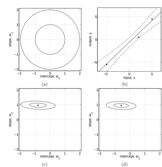
Figure 2.1: Example of Bayesian linear model f(x) = w1 +w2x with intercept w1 and slope parameter w2. Panel (a) shows the contours of the prior distribution p(w)∼ N(0, I), eq. (2.4). Panel (b) shows three training points marked by crosses. Panel (c) shows contours of the likelihoodp(y|X,w) eq. (2.3), assuming a noise level of σn= 1; note that the slope is much more “well determined” than the intercept. Panel
(d) shows the posterior,p(w|X,y) eq. (2.7); comparing the maximum of the posterior to the likelihood, we see that the intercept has been shrunk towards zero whereas the more ’well determined’ slope is almost unchanged. All contour plots give the 1 and 2 standard deviation equi-probability contours. Superimposed on the data in panel (b) are the predictive mean plus/minus two standard deviations of the (noise-free) predictive distributionp(f∗|x∗, X,y), eq. (2.9).
w. In a non-Bayesian setting the negative log prior is sometimes thought of as a penalty term, and the MAP point is known as the penalized maximum likelihood estimate of the weights, and this may cause some confusion between the two approaches. Note, however, that in the Bayesian setting the MAP estimate plays no special rˆole.3 The penalized maximum likelihood procedure 3In this case, due to symmetries in the model and posterior, it happens that the mean
of the predictive distribution is the same as the prediction at the mean of the posterior. However, this is not the case in general.
is known in this case asridge regression [Hoerl and Kennard, 1970] because of ridge regression
the effect of the quadratic penalty term 12w>Σ−1
p w from the log prior.
To make predictions for a test case we average over all possible parameter predictive distribution
values, weighted by their posterior probability. This is in contrast to non-Bayesian schemes, where a single parameter is typically chosen by some crite-rion. Thus the predictive distribution forf∗,f(x∗) atx∗is given by averaging
the output of all possible linear models w.r.t. the Gaussian posterior
p(f∗|x∗, X,y) =
Z
p(f∗|x∗,w)p(w|X,y)dw
= N 1
σ2
n
x>∗A−1Xy, x>∗A−1x∗.
(2.9)
The predictive distribution is again Gaussian, with a mean given by the poste-rior mean of the weights from eq. (2.8) multiplied by the test input, as one would expect from symmetry considerations. The predictive variance is a quadratic form of the test input with the posterior covariance matrix, showing that the predictive uncertainties grow with the magnitude of the test input, as one would expect for a linear model.
An example of Bayesian linear regression is given in Figure 2.1. Here we have chosen a 1-d input space so that the weight-space is two-dimensional and can be easily visualized. Contours of the Gaussian prior are shown in panel (a). The data are depicted as crosses in panel (b). This gives rise to the likelihood shown in panel (c) and the posterior distribution in panel (d). The predictive distribution and its error bars are also marked in panel (b).
2.1.2
Projections of Inputs into Feature Space
In the previous section we reviewed the Bayesian linear model which suffers from limited expressiveness. A very simple idea to overcome this problem is to
first project the inputs into some high dimensional space using a set of basis feature space
functions and then apply the linear model in this space instead of directly on the inputs themselves. For example, a scalar input xcould be projected into
the space of powers of x: φ(x) = (1, x, x2, x3, . . .)> to implement polynomial polynomial regression
regression. As long as the projections are fixed functions (i.e. independent of
the parameters w) the model is still linear in the parameters, and therefore linear in the parameters
analytically tractable.4 This idea is also used in classification, where a dataset
which is not linearly separable in the original data space may become linearly separable in a high dimensional feature space, see section 3.3. Application of this idea begs the question of how to choose the basis functions? As we shall demonstrate (in chapter 5), the Gaussian process formalism allows us to answer this question. For now, we assume that the basis functions are given.
Specifically, we introduce the function φ(x) which maps a D-dimensional input vector x into an N dimensional feature space. Further let the matrix
4Models with adaptive basis functions, such as e.g. multilayer perceptrons, may at first
seem like a useful extension, but they are much harder to treat, except in the limit of an infinite number of hidden units, see section 4.2.3.
Φ(X) be the aggregation of columnsφ(x) for all cases in the training set. Now the model is
f(x) = φ(x)>w, (2.10) where the vector of parameters now has lengthN. The analysis for this model is analogous to the standard linear model, except that everywhere Φ(X) is substituted forX. Thus the predictive distribution becomes
explicit feature space formulation
f∗|x∗, X,y ∼ N
1
σ2
n
φ(x∗)>A−1Φy, φ(x∗)>A−1φ(x∗)
(2.11) with Φ = Φ(X) and A = σ−2
n ΦΦ>+ Σ−p1. To make predictions using this equation we need to invert the A matrix of size N ×N which may not be convenient ifN, the dimension of the feature space, is large. However, we can rewrite the equation in the following way
alternative formulation
f∗|x∗, X,y ∼ N φ>∗ΣpΦ(K+σn2I)
−1y,
φ>∗Σpφ∗−φ>∗ΣpΦ(K+σn2I)−
1Φ>Σ
pφ∗
, (2.12)
where we have used the shorthand φ(x∗) = φ∗ and defined K = Φ>ΣpΦ.
To show this for the mean, first note that using the definitions of A and K
we have σ−n2Φ(K+σ2nI) =σ−n2Φ(Φ>ΣpΦ +σn2I) = AΣpΦ. Now multiplying through by A−1 from left and (K+σn2I)−1 from the right gives σn−2A−1Φ = ΣpΦ(K+σ2nI)−1, showing the equivalence of the mean expressions in eq. (2.11) and eq. (2.12). For the variance we use the matrix inversion lemma, eq. (A.9), setting Z−1 = Σ
p, W−1 = σ2nI and V = U = Φ therein. In eq. (2.12) we need to invert matrices of size n×n which is more convenient when n < N.
computational load
Geometrically, note that n datapoints can span at most n dimensions in the feature space.
Notice that in eq. (2.12) the feature space always enters in the form of Φ>ΣpΦ,φ>∗ΣpΦ, orφ>∗Σpφ∗; thus the entries of these matrices are invariably of
the formφ(x)>Σpφ(x0) wherexandx0are in either the training or the test sets. Let us definek(x,x0) =φ(x)>Σpφ(x0). For reasons that will become clear later we callk(·,·) acovariance function orkernel. Notice thatφ(x)>Σpφ(x0) is an
kernel
inner product (with respect to Σp). As Σpis positive definite we can define Σ1p/2 so that (Σ1p/2)2 = Σp; for example if the SVD (singular value decomposition) of Σp = U DU>, where D is diagonal, then one form for Σp1/2 is U D1/2U>. Then definingψ(x) = Σ1p/2φ(x) we obtain a simple dot product representation
k(x,x0) =ψ(x)·ψ(x0).
If an algorithm is defined solely in terms of inner products in input space then it can be lifted into feature space by replacing occurrences of those inner products byk(x,x0); this is sometimes called thekernel trick. This technique is
kernel trick
particularly valuable in situations where it is more convenient to compute the kernel than the feature vectors themselves. As we will see in the coming sections, this often leads to considering the kernel as the object of primary interest, and its corresponding feature space as having secondary practical importance.
2.2
Function-space View
An alternative and equivalent way of reaching identical results to the previous section is possible by considering inference directly in function space. We use a Gaussian process (GP) to describe a distribution over functions. Formally:
Definition 2.1 A Gaussian process is a collection of random variables, any Gaussian process
finite number of which have a joint Gaussian distribution.
A Gaussian process is completely specified by its mean function and co- covariance and mean function
variance function. We define mean functionm(x) and the covariance function
k(x,x0) of a real processf(x) as
m(x) = E[f(x)],
k(x,x0) = E[(f(x)−m(x))(f(x0)−m(x0))], (2.13)
and will write the Gaussian process as
f(x) ∼ GP m(x), k(x,x0). (2.14) Usually, for notational simplicity we will take the mean function to be zero, although this need not be done, see section 2.7.
In our case the random variables represent the value of the function f(x) at locationx. Often, Gaussian processes are defined over time, i.e. where the
index set of the random variables is time. This is not (normally) the case in index set≡
input domain
our use of GPs; here the index setX is the set of possible inputs, which could be more general, e.g. RD. For notational convenience we use the (arbitrary) enumeration of the cases in the training set to identify the random variables such thatfi ,f(xi) is the random variable corresponding to the case (xi, yi) as would be expected.
A Gaussian process is defined as a collection of random variables. Thus, the definition automatically implies aconsistency requirement, which is also
some-times known as the marginalization property. This property simply means marginalization property
that if the GP e.g. specifies (y1, y2) ∼ N(µ,Σ), then it must also specify
y1 ∼ N(µ1,Σ11) where Σ11 is the relevant submatrix of Σ, see eq. (A.6).
In other words, examination of a larger set of variables does not change the distribution of the smaller set. Notice that the consistency requirement is au-tomatically fulfilled if the covariance function specifies entries of the covariance
matrix.5 The definition does not exclude Gaussian processes with finite index finite index set
sets (which would be simply Gaussiandistributions), but these are not partic-ularly interesting for our purposes.
5Note, however, that if you instead specified e.g. a function for the entries of theinverse
covariance matrix, then the marginalization property would no longer be fulfilled, and one could not think of this as a consistent collection of random variables—this would not qualify as a Gaussian process.
A simple example of a Gaussian process can be obtained from our Bayesian
Bayesian linear model
is a Gaussian process linear regression modelf(x) =φ(x)>w with priorw∼ N(0,Σp). We have for the mean and covariance
E[f(x)] = φ(x)>E[w] = 0,
E[f(x)f(x0)] = φ(x)>E[ww>]φ(x0) = φ(x)>Σpφ(x0).
(2.15) Thusf(x) andf(x0) are jointly Gaussian with zero mean and covariance given byφ(x)>Σpφ(x0). Indeed, the function valuesf(x1), . . . , f(xn) corresponding to any number of input pointsnare jointly Gaussian, although ifN < n then this Gaussian is singular (as the joint covariance matrix will be of rankN).
In this chapter our running example of a covariance function will be the squared exponential6 (SE) covariance function; other covariance functions are discussed in chapter 4. The covariance function specifies the covariance between pairs of random variables
cov f(xp), f(xq)
= k(xp,xq) = exp −21|xp−xq|2. (2.16) Note, that the covariance between the outputs is written as a function of the inputs. For this particular covariance function, we see that the covariance is almost unity between variables whose corresponding inputs are very close, and decreases as their distance in the input space increases.
It can be shown (see section 4.3.1) that the squared exponential covariance function corresponds to a Bayesian linear regression model with an infinite number of basis functions. Indeed for every positive definite covariance function
basis functions
k(·,·), there exists a (possibly infinite) expansion in terms of basis functions (see Mercer’s theorem in section 4.3). We can also obtain the SE covariance function from the linear combination of an infinite number of Gaussian-shaped basis functions, see eq. (4.13) and eq. (4.30).
The specification of the covariance function implies a distribution over func-tions. To see this, we can draw samples from the distribution of functions evalu-ated at any number of points; in detail, we choose a number of input points,7X
∗
and write out the corresponding covariance matrix using eq. (2.16) elementwise. Then we generate a random Gaussian vector with this covariance matrix
f∗ ∼ N 0, K(X∗, X∗), (2.17)
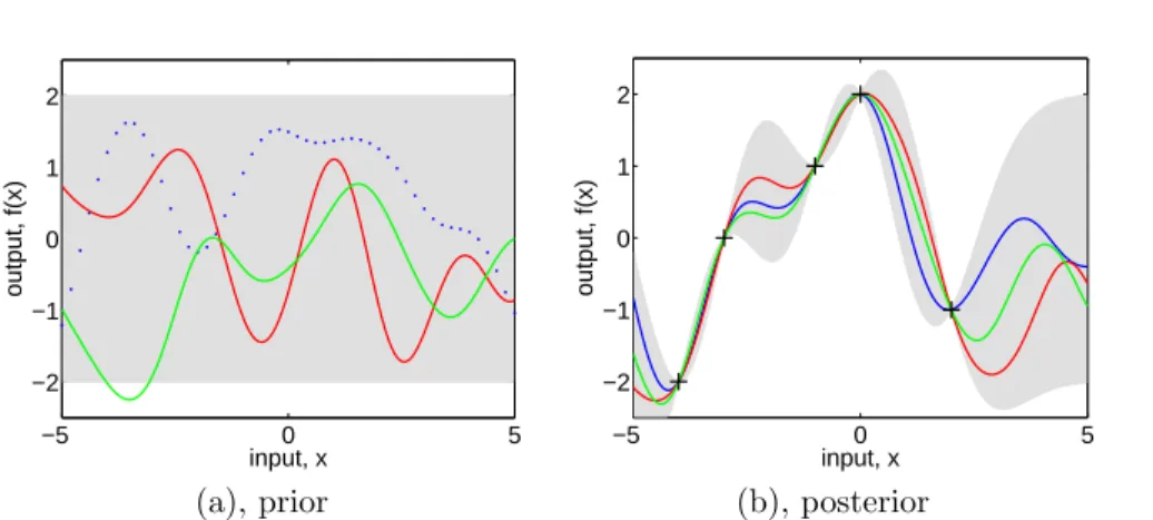
and plot the generated values as a function of the inputs. Figure 2.2(a) shows three such samples. The generation of multivariate Gaussian samples is de-scribed in section A.2.
In the example in Figure 2.2 the input values were equidistant, but this need not be the case. Notice that “informally” the functions look smooth.
smoothness
In fact the squared exponential covariance function is infinitely differentiable, leading to the process being infinitely mean-square differentiable (see section 4.1). We also see that the functions seem to have a characteristic length-scale,
characteristic
length-scale 6
Sometimes this covariance function is called the Radial Basis Function (RBF) or Gaussian; here we prefer squared exponential.
7Technically, these input points play the rˆole oftest inputsand therefore carry a subscript
−5 0 5 −2
−1 0 1 2
input, x
output, f(x)
−5 0 5
−2 −1 0 1 2
input, x
output, f(x)
(a), prior (b), posterior
Figure 2.2: Panel (a) shows three functions drawn at random from a GP prior; the dots indicate values ofy actually generated; the two other functions have (less correctly) been drawn as lines by joining a large number of evaluated points. Panel (b) shows three random functions drawn from the posterior, i.e. the prior conditioned on the five noise free observations indicated. In both plots the shaded area represents the pointwise mean plus and minus two times the standard deviation for each input value (corresponding to the 95% confidence region), for the prior and posterior respectively.
which informally can be thought of as roughly the distance you have to move in input space before the function value can change significantly, see section 4.2.1. For eq. (2.16) the characteristic length-scale is around one unit. By replacing |xp−xq|by|xp−xq|/`in eq. (2.16) for some positive constant`we could change
the characteristic length-scale of the process. Also, the overall variance of the magnitude
random function can be controlled by a positive pre-factor before the exp in eq. (2.16). We will discuss more about how such factors affect the predictions in section 2.3, and say more about how to set such scale parameters in chapter 5.
Prediction with Noise-free Observations
We are usually not primarily interested in drawing random functions from the prior, but want to incorporate the knowledge that the training data provides about the function. Initially, we will consider the simple special case where the
observations are noise free, that is we know{(xi, fi)|i = 1, . . . , n}. The joint joint prior distribution of the training outputs,f, and the test outputsf∗according to the
prior is
f f∗
∼ N
0,
K(X, X) K(X, X∗)
K(X∗, X) K(X∗, X∗)
. (2.18)
If there are n training points and n∗ test points then K(X, X∗) denotes the
n×n∗ matrix of the covariances evaluated at all pairs of training and test
points, and similarly for the other entriesK(X, X),K(X∗, X∗) andK(X∗, X).
To get the posterior distribution over functions we need to restrict this joint prior distribution to contain only those functions which agree with the observed data points. Graphically in Figure 2.2 you may think of generating functions
though this strategy would not be computationally very efficient. Fortunately, in probabilistic terms this operation is extremely simple, corresponding to con-ditioning the joint Gaussian prior distribution on the observations (see section A.2 for further details) to give
noise-free predictive distribution
f∗|X∗, X,f ∼ N K(X∗, X)K(X, X)−1f,
K(X∗, X∗)−K(X∗, X)K(X, X)−1K(X, X∗).
(2.19) Function valuesf∗ (corresponding to test inputsX∗) can be sampled from the
joint posterior distribution by evaluating the mean and covariance matrix from eq. (2.19) and generating samples according to the method described in section A.2.
Figure 2.2(b) shows the results of these computations given the five data-points marked with + symbols. Notice that it is trivial to extend these compu-tations to multidimensional inputs – one simply needs to change the evaluation of the covariance function in accordance with eq. (2.16), although the resulting functions may be harder to display graphically.
Prediction using Noisy Observations
It is typical for more realistic modelling situations that we do not have access to function values themselves, but only noisy versions thereof y =f(x) +ε.8
Assuming additive independent identically distributed Gaussian noise ε with varianceσn2, the prior on the noisy observations becomes
cov(yp, yq) = k(xp,xq) +σn2δpq or cov(y) = K(X, X) +σ2nI, (2.20) where δpq is a Kronecker delta which is one iff p = q and zero otherwise. It follows from the independence9 assumption about the noise, that a diagonal matrix10is added, in comparison to the noise free case, eq. (2.16). Introducing the noise term in eq. (2.18) we can write the joint distribution of the observed target values and the function values at the test locations under the prior as
y f∗
∼ N
0,
K(X, X) +σn2I K(X, X∗)
K(X∗, X) K(X∗, X∗)
. (2.21)
Deriving the conditional distribution corresponding to eq. (2.19) we arrive at
predictive distribution
the key predictive equations for Gaussian process regression
f∗|X,y, X∗ ∼ N ¯f∗, cov(f∗)
, where (2.22)
¯
f∗ , E[f∗|X,y, X∗] = K(X∗, X)[K(X, X) +σ2nI]
−1y, (2.23)
cov(f∗) =K(X∗, X∗)−K(X∗, X)[K(X, X) +σn2I
−1
K(X, X∗). (2.24)
8There are some situations where it is reasonable to assume that the observations are
noise-free, for example for computer simulations, see e.g. Sacks et al. [1989].
9More complicated noise models with non-trivial covariance structure can also be handled,
see section 9.2.
10Notice that the Kronecker delta is on the index of the cases, not the value of the input;
for the signal part of the covariance function the inputvalueis the index set to the random variables describing the function, for the noise part it is theidentityof the point.
Observations
Gaussian field
Inputs
y1 yc
x1 x2 x∗ xc
y∗
f1
f∗
fc
6 6 6 6
6 6 6 6 6 6 6
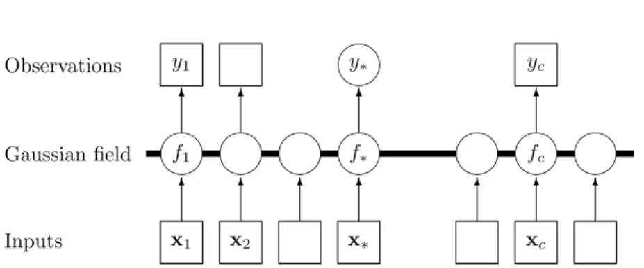
Figure 2.3: Graphical model (chain graph) for a GP for regression. Squares rep-resent observed variables and circles reprep-resent unknowns. The thick horizontal bar represents a set of fully connected nodes. Note that an observationyiis conditionally
independent of all other nodes given the corresponding latent variable,fi. Because of
the marginalization property of GPs addition of further inputs,x, latent variables,f,
andunobserved targets,y∗, does not change the distribution of any other variables.
Notice that we now have exact correspondence with the weight space view in eq. (2.12) when identifyingK(C, D) = Φ(C)>ΣpΦ(D), whereC, Dstand for
ei-therXorX∗. For any set of basis functions, we can compute the corresponding correspondence with
weight-space view
covariance function ask(xp,xq) =φ(xp)>Σpφ(xq); conversely, for every (posi-tive definite) covariance functionk, there exists a (possibly infinite) expansion in terms of basis functions, see section 4.3.
The expressions involvingK(X, X),K(X, X∗) andK(X∗, X∗) etc. can look compact notation
rather unwieldy, so we now introduce a compact form of the notation setting
K = K(X, X) and K∗ = K(X, X∗). In the case that there is only one test
pointx∗ we writek(x∗) =k∗ to denote the vector of covariances between the
test point and the n training points. Using this compact notation and for a single test pointx∗, equations 2.23 and 2.24 reduce to
¯
f∗ = k>∗(K+σ2nI)
−1y, (2.25)
V[f∗] = k(x∗,x∗)−k>∗(K+σn2I)
−1k
∗. (2.26)
Let us examine the predictive distribution as given by equations 2.25 and 2.26. predictive distribution
Note first that the mean prediction eq. (2.25) is a linear combination of
obser-vations y; this is sometimes referred to as a linear predictor. Another way to linear predictor
look at this equation is to see it as a linear combination ofnkernel functions, each one centered on a training point, by writing
¯
f(x∗) =
n
X
i=1
αik(xi,x∗) (2.27)
whereα= (K+σ2
nI)−1y. The fact that the mean prediction forf(x∗) can be
written as eq. (2.27) despite the fact that the GP can be represented in terms of a (possibly infinite) number of basis functions is one manifestation of the
representer theorem; see section 6.2 for more on this point. We can understand representer theorem
this result intuitively because although the GP defines a joint Gaussian dis-tribution over all of they variables, one for each point in the index setX, for
−5 0 5 −2
−1 0 1 2
input, x
output, f(x)
−5 0 5
−0.2 0 0.2 0.4 0.6
input, x
post. covariance, cov(f(x),f(x’))
x’=−2 x’=1 x’=3
(a), posterior (b), posterior covariance
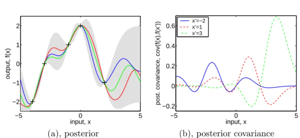
Figure 2.4: Panel (a) is identical to Figure 2.2(b) showing three random functions drawn from the posterior. Panel (b) shows the posteriorco-variance betweenf(x) and f(x0) for the same data for three different values ofx0. Note, that the covariance at close points is high, falling to zero at the training points (where there is no variance, since it is a noise-free process), then becomes negative, etc. This happens because if the smooth function happens to be less than the mean on one side of the data point, it tends to exceed the mean on the other side, causing a reversal of the sign of the covariance at the data points. Note for contrast that theprior covariance is simply of Gaussian shape and never negative.
making predictions atx∗we only care about the (n+1)-dimensional distribution
defined by the n training points and the test point. As a Gaussian distribu-tion is marginalized by just taking the relevant block of the joint covariance matrix (see section A.2) it is clear that conditioning this (n+ 1)-dimensional distribution on the observations gives us the desired result. A graphical model representation of a GP is given in Figure 2.3.
Note also that the variance in eq. (2.24) does not depend on the observed targets, but only on the inputs; this is a property of the Gaussian distribution. The variance is the difference between two terms: the first termK(X∗, X∗) is
simply the prior covariance; from that is subtracted a (positive) term, repre-senting the information the observations gives us about the function. We can very simply compute the predictive distribution of test targets y∗ by adding
noisy predictions
σ2nIto the variance in the expression for cov(f∗).
The predictive distribution for the GP model gives more than just pointwise
joint predictions
errorbars of the simplified eq. (2.26). Although not stated explicitly, eq. (2.24) holds unchanged when X∗ denotes multiple test inputs; in this case the
co-variance of the test targets are computed (whose diagonal elements are the pointwise variances). In fact, eq. (2.23) is the mean function and eq. (2.24) the covariance function of the (Gaussian) posterior process; recall the definition
posterior process
of Gaussian process from page 13. The posterior covariance in illustrated in Figure 2.4(b).
It will be useful (particularly for chapter 5) to introduce themarginal likeli-hood (or evidence)p(y|X) at this point. The marginal likelihood is the integral
input: X (inputs),y (targets),k (covariance function),σ2
n (noise level),
x∗(test input)
2: L:= cholesky(K+σ2
nI)
α:=L>\(L\y)
4: f¯∗:=k>∗α
o
predictive mean eq. (2.25)
v:=L\k∗
6: V[f∗] :=k(x∗,x∗)−v>v
o
predictive variance eq. (2.26) logp(y|X) :=−1
2y
>α−P
ilogLii−n2log 2π eq. (2.30)
8: return: ¯f∗ (mean),V[f∗] (variance), logp(y|X) (log marginal likelihood)
Algorithm 2.1: Predictions and log marginal likelihood for Gaussian process regres-sion. The implementation addresses the matrix inversion required by eq. (2.25) and (2.26) using Cholesky factorization, see section A.4. For multiple test cases lines 4-6 are repeated. The log determinant required in eq. (2.30) is computed from the Cholesky factor (for largenit may not be possible to represent the determinant itself). The computational complexity isn3/6 for the Cholesky decomposition in line 2, and n2/2 for solving triangular systems in line 3 and (for each test case) in line 5.
of the likelihood times the prior
p(y|X) =
Z
p(y|f, X)p(f|X)df. (2.28) The term marginal likelihood refers to the marginalization over the function values f. Under the Gaussian process model the prior is Gaussian, f|X ∼ N(0, K), or
logp(f|X) = −1 2f
>K−1f−1
2log|K| −
n
2log 2π, (2.29)
and the likelihood is a factorized Gaussiany|f ∼ N(f, σ2
nI) so we can make use of equations A.7 and A.8 to perform the integration yielding the log marginal likelihood
logp(y|X) = −1 2y
>(K+σ2
nI)
−1y−1
2log|K+σ 2
nI| − n
2log 2π. (2.30)
This result can also be obtained directly by observing thaty∼ N(0, K+σ2
nI). A practical implementation of Gaussian process regression (GPR) is shown in Algorithm 2.1. The algorithm uses Cholesky decomposition, instead of di-rectly inverting the matrix, since it is faster and numerically more stable, see section A.4. The algorithm returns the predictive mean and variance for noise free test data—to compute the predictive distribution for noisy test data y∗,
simply add the noise varianceσ2
n to the predictive variance off∗.
2.3
Varying the Hyperparameters
Typically the covariance functions that we use will have some free parameters. For example, the squared-exponential covariance function in one dimension has the following form
ky(xp, xq) = σf2exp − 1
2`2(xp−xq) 2
−5 0 5 −3
−2 −1 0 1 2 3
input, x
output, y
(a),`= 1
−5 0 5
−3 −2 −1 0 1 2 3
input, x
output, y
−5 0 5
−3 −2 −1 0 1 2 3
input, x
output, y
(b),`= 0.3 (c), `= 3
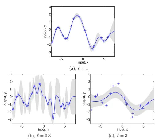
Figure 2.5: (a) Data is generated from a GP with hyperparameters (`, σf, σn) =
(1,1,0.1), as shown by the + symbols. Using Gaussian process prediction with these hyperparameters we obtain a 95% confidence region for the underlying function f (shown in grey). Panels (b) and (c) again show the 95% confidence region, but this time for hyperparameter values (0.3,1.08,0.00005) and (3.0,1.16,0.89) respectively.
The covariance is denotedky as it is for the noisy targets yrather than for the underlying function f. Observe that the length-scale`, the signal variance σ2
f and the noise varianceσn2 can be varied. In general we call the free parameters
hyperparameters
hyperparameters.11
In chapter 5 we will consider various methods for determining the hyperpa-rameters from training data. However, in this section our aim is more simply to explore the effects of varying the hyperparameters on GP prediction. Consider the data shown by + signs in Figure 2.5(a). This was generated from a GP with the SE kernel with (`, σf, σn) = (1,1,0.1). The figure also shows the 2 standard-deviation error bars for the predictions obtained using these values of the hyperparameters, as per eq. (2.24). Notice how the error bars get larger for input values that are distant from any training points. Indeed if the x-axis
11We refer to the parameters of the covariance function as hyperparameters to emphasize
that they are parameters of a non-parametric model; in accordance with the weight-space view, section 2.1, the parameters (weights) of the underlying parametric model have been integrated out.
were extended one would see the error bars reflect the prior standard deviation of the processσf away from the data.
If we set the length-scale shorter so that ` = 0.3 and kept the other pa-rameters the same, then generating from this process we would expect to see plots like those in Figure 2.5(a) except that the x-axis should be rescaled by a factor of 0.3; equivalently if the same x-axis was kept as in Figure 2.5(a) then a sample function would look much more wiggly.
If we make predictions with a process with `= 0.3 on the data generated too short length-scale
from the`= 1 process then we obtain the result in Figure 2.5(b). The remaining two parameters were set by optimizing the marginal likelihood, as explained in chapter 5. In this case the noise parameter is reduced to σn = 0.00005 as the greater flexibility of the “signal” means that the noise level can be reduced. This can be observed at the two datapoints nearx= 2.5 in the plots. In Figure 2.5(a) (` = 1) these are essentially explained as a similar function value with differing noise. However, in Figure 2.5(b) (`= 0.3) the noise level is very low, so these two points have to be explained by a sharp variation in the value of the underlying functionf. Notice also that the short length-scale means that the error bars in Figure 2.5(b) grow rapidly away from the datapoints.
In contrast, we can set the length-scale longer, for example to`= 3, as shown too long length-scale
in Figure 2.5(c). Again the remaining two parameters were set by optimizing the marginal likelihood. In this case the noise level has been increased toσn = 0.89 and we see that the data is now explained by a slowly varying function with a lot of noise.
Of course we can take the position of a quickly-varying signal with low noise, or a slowly-varying signal with high noise to extremes; the former would give rise to a white-noise process model for the signal, while the latter would give rise to a constant signal with added white noise. Under both these models the datapoints produced should look like white noise. However, studying Figure 2.5(a) we see that white noise is not a convincing model of the data, as the sequence ofy’s does not alternate sufficiently quickly but has correlations due to the variability of
the underlying function. Of course this is relatively easy to see in one dimension, model comparison
but methods such as the marginal likelihood discussed in chapter 5 generalize to higher dimensions and allow us to score the various models. In this case the marginal likelihood gives a clear preference for (`, σf, σn) = (1,1,0.1) over the other two alternatives.
2.4
Decision Theory for Regression
In the previous sections we have shown how to compute predictive distributions for the outputsy∗corresponding to the novel test inputx∗. The predictive
dis-tribution is Gaussian with mean and variance given by eq. (2.25) and eq. (2.26). In practical applications, however, we are often forced to make a decision about
how to act, i.e. we need a point-like prediction which is optimal in some sense. optimal predictions
penalty) incurred by guessing the valueyguess when the true value isytrue. For
example, the loss function could equal the absolute deviation between the guess and the truth.
Notice that we computed the predictive distribution without reference to the loss function. In non-Bayesian paradigms, the model is typically trained
non-Bayesian paradigm
by minimizing the empirical risk (or loss). In contrast, in the Bayesian setting
Bayesian paradigm
there is a clear separation between the likelihood function (used for training, in addition to the prior) and the loss function. The likelihood function describes how the noisy measurements are assumed to deviate from the underlying noise-free function. The loss function, on the other hand, captures the consequences of making a specific choice, given an actual true state. The likelihood and loss function need not have anything in common.12
Our goal is to make the point predictionyguesswhich incurs the smallest loss,
but how can we achieve that when we don’t knowytrue? Instead, we minimize
theexpected loss orrisk, by averaging w.r.t. our model’s opinion as to what the
expected loss, risk
truth might be ˜
RL(yguess|x∗) =
Z
L(y∗, yguess)p(y∗|x∗,D)dy∗. (2.32)
Thus our best guess, in the sense that it minimizes the expected loss, is
yoptimal|x∗ = argmin
yguess
˜
RL(yguess|x∗). (2.33)
In general the value ofyguessthat minimizes the risk for the loss function|yguess− absolute error loss
y∗| is the median of p(y∗|x∗,D), while for the squared loss (yguess−y∗)2 it is
squared error loss
the mean of this distribution. When the predictive distribution is Gaussian the mean and the median coincide, and indeed for any symmetric loss function and symmetric predictive distribution we always getyguess as the mean of the
predictive distribution. However, in many practical problems the loss functions can be asymmetric, e.g. in safety critical applications, and point predictions may be computed directly from eq. (2.32) and eq. (2.33). A comprehensive treatment of decision theory can be found in Berger [1985].
2.5
An Example Application
In this section we use Gaussian process regression to learn the inverse dynamics of a seven degrees-of-freedom SARCOS anthropomorphic robot arm. The task
robot arm
is to map from a 21-dimensional input space (7 joint positions, 7 joint velocities, 7 joint accelerations) to the corresponding 7 joint torques. This task has pre-viously been used to study regression algorithms by Vijayakumar and Schaal [2000], Vijayakumar et al. [2002] and Vijayakumar et al. [2005].13 Following 12Beware of fallacious arguments like: a Gaussian likelihood implies a squared error loss
function.
this previous work we present results below on just one of the seven mappings, from the 21 input variables to the first of the seven torques.
One might ask why it is necessary tolearn this mapping; indeed there exist why learning?
physics-based rigid-body-dynamics models which allow us to obtain the torques from the position, velocity and acceleration variables. However, the real robot arm is actuated hydraulically and is rather lightweight and compliant, so the assumptions of the rigid-body-dynamics model are violated (as we see below). It is worth noting that the rigid-body-dynamics model is nonlinear, involving trigonometric functions and squares of the input variables.
An inverse dynamics model can be used in the following manner: a planning module decides on a trajectory that takes the robot from its start to goal states, and this specifies the desired positions, velocities and accelerations at each time. The inverse dynamics model is used to compute the torques needed to achieve this trajectory and errors are corrected using a feedback controller.
The dataset consists of 48,933 input-output pairs, of which 44,484 were used as a training set and the remaining 4,449 were used as a test set. The inputs were linearly rescaled to have zero mean and unit variance on the training set. The outputs were centered so as to have zero mean on the training set.
Given a prediction method, we can evaluate the quality of predictions in several ways. Perhaps the simplest is the squared error loss, where we compute the squared residual (y∗−f¯(x∗))2 between the mean prediction and the target
at each test point. This can be summarized by the mean squared error (MSE), MSE
by averaging over the test set. However, this quantity is sensitive to the overall scale of the target values, so it makes sense to normalize by the variance of the targets of the test cases to obtain thestandardized mean squared error (SMSE).
This causes the trivial method of guessing the mean of the training targets to SMSE
have a SMSE of approximately 1.
Additionally if we produce a predictive distribution at each test input we can evaluate the negative log probability of the target under the model.14 As
GPR produces a Gaussian predictive density, one obtains −logp(y∗|D,x∗) =
1
2log(2πσ
2
∗) +
(y∗−f¯(x∗))2
2σ2
∗
, (2.34)
where the predictive variance σ2
∗ for GPR is computed as σ∗2 = V(f∗) +σ2n, whereV(f∗) is given by eq. (2.26); we must include the noise varianceσn2 as we are predicting the noisy targety∗. This loss can be standardized by subtracting
the loss that would be obtained under the trivial model which predicts using a Gaussian with the mean and variance of the training data. We denote this
the standardized log loss (SLL). The mean SLL is denoted MSLL. Thus the MSLL
MSLL will be approximately zero for simple methods and negative for better methods.
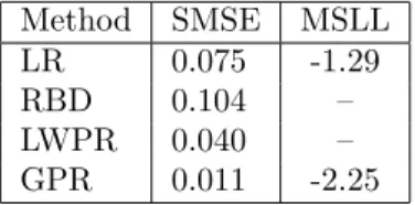
A number of models were tested on the data. A linear regression (LR) model provides a simple baseline for the SMSE. By estimating the noise level from the
Method SMSE MSLL
LR 0.075 -1.29
RBD 0.104 –
LWPR 0.040 –
GPR 0.011 -2.25
Table 2.1: Test results on the inverse dynamics problem for a number of different methods. The “–” denotes a missing entry, caused by two methods not producing full predictivedistributions, so MSLL could not be evaluated.
residuals on the training set one can also obtain a predictive variance and thus get a MSLL value for LR. The rigid-body-dynamics (RBD) model has a number of free parameters; these were estimated by Vijayakumar et al. [2005] using a least-squares fitting procedure. We also give results for the locally weighted projection regression (LWPR) method of Vijayakumar et al. [2005] which is an on-line method that cycles through the dataset multiple times. For the GP models it is computationally expensive to make use of all 44,484 training cases due to theO(n3) scaling of the basic algorithm. In chapter 8 we present several different approximate GP methods for large datasets. The result given in Table 2.1 was obtained with the subset of regressors (SR) approximation with a subset size of 4096. This result is taken from Table 8.1, which gives full results of the various approximation methods applied to the inverse dynamics problem. The squared exponential covariance function was used with a separate length-scale parameter for each of the 21 input dimensions, plus the signal and noise variance parameters σ2
f andσ
2
n. These parameters were set by optimizing the marginal likelihood eq. (2.30) on a subset of the data (see also chapter 5).
The results for the various methods are presented in Table 2.1. Notice that the problem is quite non-linear, so the linear regression model does poorly in comparison to non-linear methods.15 The non-linear method LWPR improves
over linear regression, but is outperformed by GPR.
2.6
Smoothing, Weight Functions and
Equiva-lent Kernels
Gaussian process regression aims to reconstruct the underlying signal f by removing the contaminating noiseε. To do this it computes a weighted average of the noisy observationsyas ¯f(x∗) =k(x∗)>(K+σ2nI)−1y; as ¯f(x∗) is alinear
combination of the y values, Gaussian process regression is alinear smoother
linear smoother
(see Hastie and Tibshirani [1990, sec. 2.8] for further details). In this section we study smoothing first in terms of a matrix analysis of the predictions at the training points, and then in terms of the equivalent kernel.
15It is perhaps surprising that RBD does worse than linear regression. However, Stefan
Schaal (pers. comm., 2004) states that the RBD parameters were optimized on a very large dataset, of which the training data used here is subset, and if the RBD model were optimized w.r.t. this training set one might well expect it to outperform linear regression.
The predicted mean values ¯f at the training points are given by ¯
f = K(K+σ2nI)−1y. (2.35) Let K have the eigendecomposition K = Pn
i=1λiuiu>i , where λi is the ith eigendecomposition eigenvalue and ui is the corresponding eigenvector. As K is real and
sym-metric positive semidefinite, its eigenvalues are real and non-negative, and its eigenvectors are mutually orthogonal. Lety=Pn
i=1γiui for some coefficients
γi=u>i y. Then
¯
f = n
X
i=1
γiλi
λi+σ2n
ui. (2.36)
Notice that ifλi/(λi+σ2n)1 then the component inyalonguiis effectively eliminated. For most covariance functions that are used in practice the eigen-values are larger for more slowly varying eigenvectors (e.g. fewer zero-crossings) so that this means that high-frequency components in y are smoothed out.
The effective number of parameters or degrees of freedom of the smoother is degrees of freedom
defined as tr(K(K+σn2I)−1) =Pn
i=1λi/(λi+σ2n), see Hastie and Tibshirani [1990, sec. 3.5]. Notice that this counts the number of eigenvectors which are not eliminated.
We can define a vector of functions h(x∗) = (K+σn2I)−1k(x∗). Thus we
have ¯f(x∗) = h(x∗)>y, making it clear that the mean prediction at a point
x∗ is a linear combination of the target values y. For a fixed test point x∗,
h(x∗) gives the vector of weights applied to targetsy. h(x∗) is called theweight
function[Silverman, 1984]. As Gaussian process regression is a linear smoother, weight function
the weight function does not depend on y. Note the difference between a linearmodel, where the prediction is a linear combination of theinputs, and a linearsmoother, where the prediction is a linear combination of the training set targets.
Understanding the form of the weight function is made complicated by the matrix inversion ofK+σn2Iand the fact thatKdepends on the specific locations of thendatapoints. Idealizing the situation one can consider the observations to be “smeared out” in x-space at some density of observations. In this case analytic tools can be brought to bear on the problem, as shown in section 7.1. By analogy to kernel smoothing, Silverman [1984] called the idealized weight
function theequivalent kernel; see also Girosi et al. [1995, sec. 2.1]. equivalent kernel
A kernel smoother centres a kernel function16 κon x∗ and then computes kernel smoother
κi=κ(|xi−x∗|/`) for each data point (xi, yi), where` is a length-scale. The Gaussian is a commonly used kernel function. The prediction for f(x∗) is
computed as ˆf(x∗) =Pni=1wiyi where wi = κi/P n
j=1κj. This is also known as the Nadaraya-Watson estimator, see e.g. Scott [1992, sec. 8.1].
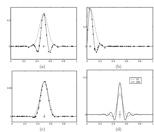
The weight function and equivalent kernel for a Gaussian process are illus-trated in Figure 2.6 for a one-dimensional input variablex. We have used the squared exponential covariance function and have set the length-scale`= 0.0632 (so that`2 = 0.004). There are n= 50 training points spaced randomly along
0 0.2 0.4 0.6 0.8 1 0
0.2
0 0.2 0.4 0.6 0.8 1 0
0.2
(a) (b)
0 0.2 0.4 0.6 0.8 1 0
0.05
0 0.2 0.4 0.6 0.8 1 0
0.1
10 250
(c) (d)
Figure 2.6: Panels (a)-(c) show the weight function h(x∗) (dots) corresponding to the n = 50 training points, the equivalent kernel (solid) and the original squared exponential kernel (dashed). Panel (d) shows the equivalent kernels for two different data densities. See text for further details. The small cross at the test point is to scale in all four plots.
thex-axis. Figures 2.6(a) and 2.6(b) show the weight function and equivalent kernel forx∗= 0.5 andx∗= 0.05 respectively, forσ2n= 0.1. Figure 2.6(c) is also forx∗= 0.5 but usesσ2n= 10. In each case the dots correspond to the weight functionh(x∗) and the solid line is the equivalent kernel, whose construction is
explained below. The dashed line shows a squared exponential kernel centered on the test point, scaled to have the same height as the maximum value in the equivalent kernel. Figure 2.6(d) shows the variation in the equivalent kernel as a function ofn, the number of datapoints in the unit interval.
Many interesting observations can be made from these plots. Observe that the equivalent kernel has (in general) a shape quite different to the original SE kernel. In Figure 2.6(a) the equivalent kernel is clearly oscillatory (with negative sidelobes) and has a higher spatial frequency than the original kernel. Figure 2.6(b) shows similar behaviour although due to edge effects the equivalent kernel is truncated relative to that in Figure 2.6(a). In Figure 2.6(c) we see that at higher noise levels the negative sidelobes are reduced and the width of the equivalent kernel is similar to the original kernel. Also note that the overall height of the equivalent kernel in (c) is reduced compared to that in (a) and
(b)—it averages over a wider area. The more oscillatory equivalent kernel for lower noise levels can be understood in terms of the eigenanalysis above; at higher noise levels only the large λ(slowly varying) components of y remain, while for smaller noise levels the more oscillatory components are also retained. In Figure 2.6(d) we have plotted the equivalent kernel for n= 10 and n= 250 datapoints in [0,1]; notice how the width of the equivalent kernel decreases asnincreases. We discuss this behaviour further in section 7.1.
The plots of equivalent kernels in Figure 2.6 were made by using a dense grid ofngrid points on [0,1] and then computing the smoother matrixK(K+
σ2 gridI)
−1. Each row of this matrix is the equivalent kernel at the appropriate
location. However, in order to get the scaling right one has to set σ2 grid =
σ2
nngrid/n; for ngrid > n this means that the effective variance at each of the
ngrid points is larger, but as there are correspondingly more points this effect
cancels out. This can be understood by imagining the situation if there were
ngrid/n independent Gaussian observations with variance σgrid2 at a single x
-position; this would be equivalent to one Gaussian observation with variance
σ2n. In effect then observations have been smoothed out uniformly along the interval. The form of the equivalent kernel can be obtained analytically if we go to the continuum limit and look to smooth a noisy function. The relevant theory and some example equivalent kernels are given in section 7.1.
2.7
Incorporating Explicit Basis Functions
∗
It is common but by no means necessary to consider GPs with a zero mean func-tion. Note that this is not necessarily a drastic limitation, since the mean of the posterior process is not confined to be zero. Yet there are several reasons why one might wish to explicitly model a mean function, including interpretability of the model, convenience of expressing prior information and a number of an-alytical limits which we will need in subsequent chapters. The use of explicit basis functions is a way to specify a non-zero mean over functions, but as we will see in this section, one can also use them to achieve other interesting effects.
Using a fixed (deterministic) mean function m(x) is trivial: Simply apply fixed mean function
the usual zero mean GP to the difference between the observations and the fixed mean function. With
f(x) ∼ GP m(x), k(x,x0)
, (2.37)
the predictive mean becomes ¯
f∗ = m(X∗) +K(X∗, X)Ky−1(y−m(X)), (2.38) where Ky = K+σn2I, and the predictive variance remains unchanged from eq. (2.24).
However, in practice it can often be difficult to specify a fixed mean function. In many cases it may be more convenient to specify a few fixed basis functions,
whose coefficients,β, are to be inferred from the data. Consider
stochastic mean function
g(x) = f(x) +h(x)>β, where f(x) ∼ GP 0, k(x,x0)
, (2.39)
heref(x) is a zero mean GP,h(x) are a set of fixed basis functions, andβare additional parameters. This formulation expresses that the data is close to a global linear model with the residuals being modelled by a GP. This idea was explored explicitly as early as 1975 by Blight and Ott [1975], who used the GP to model the residuals from a polynomial regression, i.e.h(x) = (1, x, x2, . . .).
polynomial regression
When fitting the model, one could optimize over the parametersβjointly with the hyperparameters of the covariance function. Alternatively, if we take the prior on β to be Gaussian, β ∼ N(b, B), we can also integrate out these parameters. Following O’Hagan [1978] we obtain another GP
g(x) ∼ GP h(x)>b, k(x,x0) +h(x)>Bh(x0)
, (2.40)
now with an added contribution in the covariance function caused by the un-certainty in the parameters of the mean. Predictions are made by plugging the mean and covariance functions ofg(x) into eq. (2.39) and eq. (2.24). After rearranging, we obtain
¯
g(X∗) = H∗>β¯ +K∗>Ky−1(y−H>β¯) = ¯f(X∗) +R>β¯,
cov(g∗) = cov(f∗) +R>(B−1+HKy−1H
>)−1R, (2.41)
where theH matrix collects theh(x) vectors for all training (andH∗ all test)
cases, ¯β= (B−1+HK−1
y H>)−1(HKy−1y+B−1b), and R=H∗−HKy−1K∗.
Notice the nice interpretation of the mean expression, eq. (2.41) top line: ¯β is the mean of the global linear model parameters, being a compromise between the data term and prior, and the predictive mean is simply the mean linear output plus what the GP model predicts from the residuals. The covariance is the sum of the usual covariance term and a new non-negative contribution.
Exploring the limit of the above expressions as the prior on the β param-eter becomes vague, B−1 →O (where O is the matrix of zeros), we obtain a predictive distribution which is independent ofb
¯
g(X∗) = ¯f(X∗) +R>β¯,
cov(g∗) = cov(f∗) +R>(HKy−1H>)−
1R, (2.42)
where the limiting ¯β = (HK−1
y H>)−1HKy−1y. Notice that predictions under the limitB−1→Oshould not be implemented na¨ıvely by plugging the modified
covariance function from eq. (2.40) into the standard prediction equations, since the entries of the covariance function tend to infinity, thus making it unsuitable for numerical implementation. Instead eq. (2.42) must be used. Even if the non-limiting case is of interest, eq. (2.41) is numerically preferable to a direct implementation based on eq. (2.40), since the global linear part will often add some very large eigenvalues to the covariance matrix, affecting its condition number.
2.7.1
Marginal Likelihood
In this short section we briefly discuss the marginal likelihood for the model with a Gaussian priorβ∼ N(b, B) on the explicit parameters from eq. (2.40), as this will be useful later, particularly in section 6.3.1. We can express the marginal likelihood from eq. (2.30) as
logp(y|X,b, B) = −1 2(H
>b−y)>(K
y+H>BH)−1(H>b−y) −1
2log|Ky+H>BH| −n2log 2π,
(2.43) where we have included the explicit mean. We are interested in exploring the limit whereB−1→O, i.e. when the prior is vague. In this limit the mean of the
prior is irrelevant (as was the case in eq. (2.42)), so without loss of generality (for the limiting case) we assume for now that the mean is zero,b=0, giving
logp(y|X,b=0, B) = −1 2y
>K−1
y y+
1 2y
>Cy
−1
2log|Ky| − 1
2log|B| − 1
2log|A| −
n
2log 2π,
(2.44) where A = B−1+HKy−1H> and C =Ky−1H>A−1HKy−1 and we have used the matrix inversion lemma, eq. (A.9) and eq. (A.10).
We now explore the behaviour of the log marginal likelihood in the limit of vague priors onβ. In this limit the variances of the Gaussian in the directions spanned by columns of H> will become infinite, and it is clear that this will require special treatment. The log marginal likelihood consists of three terms: a quadratic form in y, a log determinant term, and a term involving log 2π. Performing an eigendecomposition of the covariance matrix we see that the contributions to quadratic form term from the infinite-variance directions will be zero. However, the log determinant term will tend to minus infinity. The standard solution [Wahba, 1985, Ansley and Kohn, 1985] in this case is to project y onto the directions orthogonal to the span of H> and compute the marginal likelihood in this subspace. Let the rank of H> be m. Then as shown in Ansley and Kohn [1985] this means that we must discard the terms −1
2log|B| −
m
2 log 2πfrom eq. (2.44) to give
logp(y|X) = −1 2y
>K−1
y y+
1 2y
>Cy−1
2log|Ky| − 1
2log|A| −
n−m
2 log 2π,
(2.45) whereA=HK−1
y H> and C=Ky−1H>A−1HKy−1.
2.8
History and Related Work
Prediction with Gaussian processes is certainly not a very recent topic,
espe-cially for time series analysis; the basic theory goes back at least as far as the time series
work of Wiener [1949] and Kolmogorov [1941] in the 1940’s. Indeed Lauritzen [1981] discusses relevant work by the Danish astronomer T. N. Thiele dating from 1880.
Gaussian process prediction is also well known in the geostatistics field (see,
geostatistics
e.g. Matheron, 1973; Journel and Huijbregts, 1978) where it is known as krig-ing,17 and in meteorology [Thompson, 1956, Daley, 1991] although this litera-kriging
ture naturally has focussed mostly on two- and three-dimensional input spaces. Whittle [1963, sec. 5.4] also suggests the use of such methods for spatial pre-diction. Ripley [1981] and Cressie [1993] provide useful overviews of Gaussian process prediction in spatial statistics.
Gradually it was realized that Gaussian process prediction could be used in a general regression context. For example O’Hagan [1978] presents the general theory as given in our equations 2.23 and 2.24, and applies it to a number of one-dimensional regression problems. Sacks et al. [1989] describe GPR in the context of computer experiments (where the observationsyare noise free) and
computer experiments
discuss a number of interesting directions such as the optimization of parameters in the covariance function (see our chapter 5) and experimental design (i.e. the choice ofx-points that provide most information on f). The authors describe a number of computer simulations that were modelled, including an example where the response variable was the clock asynchronization in a circuit and the inputs were six transistor widths. Santner et al. [2003] is a recent book on the use of GPs for the design and analysis of computer experiments.
Williams and Rasmussen [1996] described Gaussian process regression in
machine learning
a machine learning context, and described optimization of the parameters in the covariance function, see also Rasmussen [1996]. They were inspired to use Gaussian process by the connection to infinite neural networks as described in section 4.2.3 and in Neal [1996]. The “kernelization” of linear ridge regression described above is also known askernel ridge regressionsee e.g. Saunders et al. [1998].
Relationships between Gaussian process prediction and regularization the-ory, splines, support vector machines (SVMs) and relevance vector machines (RVMs) are discussed in chapter 6.
2.9
Exercises
1. Replicate the generation of random functions from Figure 2.2. Use a regular (or random) grid of scalar inputs and the covariance function from eq. (2.16). Hints on how to generate random samples from multi-variate Gaussian distributions are given in section A.2. Invent some training data points, and make random draws from the resulting GP posterior using eq. (2.19).
2. In eq. (2.11) we saw that the predictive variance atx∗ under the feature
space regression model was var(f(x∗)) = φ(x∗)>A−1φ(x∗). Show that
cov(f(x∗), f(x0∗)) =φ(x∗)>A−1φ(x0∗). Check that this is compatible with
the expression given in eq. (2.24).
3. The Wiener process is defined for x ≥ 0 and has f(0) = 0. (See sec-tion B.2.1 for further details.) It has mean zero and a non-stasec-tionary covariance function k(x, x0) = min(x, x0). If we condition on the Wiener process passing throughf(1) = 0 we obtain a process known as the Brow-nian bridge (or tied-down Wiener process). Show that this process has covariancek(x, x0) = min(x, x0)−xx0 for 0≤x, x0≤1 and mean 0. Write a computer program to draw samples from this process at a finite grid of
xpoints in [0,1].
4. Let varn(f(x∗)) be the predictive variance of a Gaussian process
regres-sion model atx∗ given a dataset of sizen. The corresponding predictive
variance using a dataset of only the first n−1 training points is de-noted varn−1(f(x∗)). Show that varn(f(x∗))≤varn−1(f(x∗)), i.e. that
the predictive variance atx∗ cannot increase as more training data is
ob-tained. One way to approach this problem is to use the partitioned matrix equations given in section A.3 to decompose varn(f(x∗)) = k(x∗,x∗)−
k>∗(K+σ2
nI)−1k∗.An alternative information theoretic argument is given
in Williams and Vivarelli [2000]. Note that while this conclusion is true for Gaussian process priors and Gaussian noise models it does not hold generally, see Barber and Saad [1996].