Where Value Meets Values: The Economic Impact of Community Colleges

(1)

Where Value Meets Values: The

Economic Impact of Community

Colleges

Analysis of the Economic Impact and Return on Investment of

Education

February 2014

Economic Modeling Specialists Intl. 1187 Alturas Dr.

Moscow, ID 83843 208-883-3500

(2)

Acknowledgments

Economic Modeling Specialists International (EMSI) gratefully acknowledges the excellent support of the staff at the American Association of Community Colleges (AACC) in making this study possible. Special thanks go to Dr. Walter G. Bumphus, President and CEO, who approved the study; and to Dr. Angel M. Royal, Chief of Staff, and Kent A. Phillippe, Associate Vice President, Research and Student Success. Any errors in the report are the responsibility of EMSI and not of any of the above-mentioned institutions or individuals.

(5)

Preface

Since 2002, Economic Modeling Specialists International (EMSI) has helped address a widespread need in the U.S., Canada, the U.K., and Australia to demonstrate the impact of education. To date we have conducted more than 1,200 economic impact studies for educational institutions in the U.S. and internationally. Along the way we have worked to continuously update and improve the model to ensure that it conforms to best practices and stays relevant in today’s economy.

The present study reflects the latest version of our model, representing the most up-to-date theory and practices for conducting human capital economic impact analysis. Among the most vital departures from EMSI’s previous economic model is the conversion from traditional Leontief input-output multipliers to those generated by EMSI’s multi-regional Social Accounting Matrix (SAM). Though Leontief multipliers are based on sound theory, they are less comprehensive and adaptable than SAM multipliers. Moving to the more robust SAM framework allows us to increase the level of sectoral detail in the model and remove any aggregation error that may have occurred under the previous framework.

Another major change in the model is the replacement of John Parr’s development index with a proprietary mapping of instructional programs to detailed industries. The Parr index was a significant move forward when we first applied it in 2000 to approximate the industries where students were most likely to find employment after leaving college. Now, by mapping program completers to detailed industries, we can move from an approach based on assumptions to one based on actual occupations for which students are trained.

The new model also reflects significant changes to the calculation of the alternative education variable. This variable addresses the counterfactual scenario of what would have occurred if the publicly-funded community colleges in the U.S. did not exist, leaving the students to obtain an education elsewhere. The previous model used a small-sample regression analysis to estimate the variable. The current model goes further and measures the distance between institutions and the associated differences in tuition prices to determine the change in the students’ demand for education. This methodology is a more robust approach than the regression analysis and significantly improves our estimate of alternative education opportunities.

These and other changes mark a considerable upgrade to the EMSI college impact model. With the SAM we have a more detailed view of the economy, enabling us to more accurately determine economic impacts. Many of our former assumptions have been replaced with observed data, as exemplified by the program-to-industry mapping and the revision to the alternative education variable. Further, we have researched the latest sources in order to update the background data with the most up-to-date data and information. We encourage our readers to approach us directly with any questions or comments they may have about the study so that we can continue to improve our model and keep the public dialogue open about the positive impacts of education.

(6)

Introduction

America’s community colleges create value in many ways. With a wide range of program offerings, community colleges play a key role in helping students achieve their individual potential and develop the skills they need in order to have a fulfilling and prosperous career. Community colleges also provide an excellent environment for students to meet new people and make friends, while participation in college courses improves the students’ self-confidence and promotes their mental health. These social and employment-related benefits have a positive influence on the health and well-being of individuals.

However, the contribution of America’s community colleges consists of more than solely influencing the lives of students. The colleges’ program offerings support a range of industry sectors in the U.S. and supply employers with the skilled workers they need to make their businesses more productive. The expenditures of the colleges and their international students further support the national economy through the output and employment generated by businesses. Lastly, and just as importantly, the benefits of community colleges extend as far as the national treasury in terms of increased tax receipts and decreased public sector costs.

Objective of the report

This report assesses the impact of America’s public community colleges on the national economy and the return on investment for the colleges’ key stakeholder groups: students, society, and taxpayers. Our approach is twofold. We begin with an economic impact analysis of the colleges using a specialized Social Accounting Matrix (SAM) model to calculate the additional income created in the U.S. as a result of increased consumer spending and the added skills of students. Results of the economic impact analysis are broken out according to the following three effects: 1) impact of the colleges’ provision to international students, 2) impact of the living expenses of international students, and 3) impact of the skills acquired by former students that are still active in the U.S. workforce.

The second component of the study is a standard investment analysis to determine how money spent on community colleges performs as an investment over time. The investors in this case are students, society, and taxpayers, all of whom pay a certain amount in costs to support the educational activities at the colleges. The students’ investment consists of their out-of-pocket expenses and the opportunity cost of attending college as opposed to working. Society invests in education by forgoing the services that it would have received had government not funded the colleges and the business output that it would have enjoyed had students been employed instead of studying. Taxpayers contribute their investment through government funding.

In return for these investments, students receive a lifetime of higher incomes, society benefits from an enlarged national economy and a reduced demand for social services, and taxpayers benefit from

(7)

an expanded tax base and a collection of public sector savings. To determine the feasibility of the investment, the model projects benefits into the future, discounts them back to their present value, and compares them to their present value costs. Results of the investment analysis for students, society, and taxpayers are displayed in the following five ways: 1) net present value of benefits, 2) rate of return, 3) benefit-cost ratio, 4) return on investment, and 5) payback period.

A wide array of data and assumptions are used in the study based on a number of sources, including the latest academic and financial data for 1,025 public and tribal two-year college entities that report to the Integrated Postsecondary Education Data System (IPEDS), industry and employment data from the U.S. Bureau of Labor Statistics and the U.S. Census Bureau, observations from approximately 200 sample colleges for which EMSI has recently conducted individual impact analyses, outputs of EMSI’s SAM model, and a variety of published materials relating education to social behavior. The study aims to apply a conservative methodology and follows standard practice using only the most recognized indicators of investment effectiveness and economic impact.

Notes of importance

There are two notes of importance that readers should bear in mind when reviewing the findings presented in this report. First, this report is not intended to be a vehicle for comparing or ranking publicly-funded institutions. Other studies comparing the gains in income and social benefits of one institution relative to another address such questions more directly and in greater detail. Our intent is simply to provide college management teams and stakeholders with pertinent information should questions arise about the extent to which community colleges impact the national economy and generate a return on investment. Although the methodology used to derive results for individual colleges is similar to the methodology applied in this study, differences between results do not necessarily indicate that some colleges are doing a better job than others. Results are a reflection of location, student body profile, and other factors that have little or nothing to do with the relative efficiency of the community colleges. For this reason, comparing results between colleges or using the data to rank colleges is strongly discouraged.

Second, this report is useful in establishing a benchmark for future analysis, but it is limited in its ability to put forward recommendations on what community colleges can do next. The implied assumption is that colleges can effectively improve the results if they increase the number of students they serve, help students to achieve their educational goals, and remain responsive to employer needs in order to ensure that students find meaningful jobs after exiting. Establishing a strategic plan for achieving these goals, however, is not the purpose of this report.

Key findings

The results of this study show that America’s community colleges have a significant positive impact on the national economy and generate a return on investment for their main stakeholder groups: students, society, and taxpayers. Using a two-pronged approach that involves an economic impact

(8)

analysis and an investment analysis, we calculate the benefits to each of these groups. Key findings of the study are as follows:

Impact on national economy

• _{The enhanced skills and abilities of community college students bolster the output of U.S.}

employers, leading to higher income and a more robust economy. The accumulated contribution of former students who were employed in the U.S. workforce in 2012 amounted to $806.4 billion in added income in the national economy.

• _{A total of} _146,500_{international students relocated to the U.S. to attend America’s}

community colleges in 2012. These students paid $1.2 billion to the community colleges to cover the cost of their tuition and fees and purchase books and supplies. The net impact of these expenses was approximately $1.5 billion in added national income.

• _{International students also spent money to purchase groceries, rent accommodation, pay for}

transport, attend sporting events, and so on. These expenditures supported U.S. businesses and added approximately $1.1 billion in income to the national economy.

• _{The total effect of America’s community colleges on the U.S. economy in 2012 was}_$809

billion, approximately equal to 5.4% of the nation’s Gross Domestic Product.

Return on investment to students, society, and taxpayers

• _{Students paid a total of}_{$18.7 billion}_{to cover the cost of tuition, fees, books, and supplies at}

America’s community colleges in 2012. They also forwent $78.7 billion in earnings that they would have generated had they been working instead of learning.

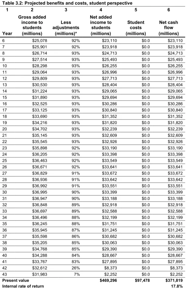
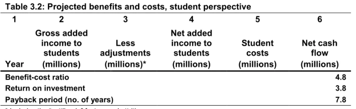
• _{In return for the monies invested in their college education, students will receive a present}

value of $469.3 billion in increased earnings over their working lives. This translates to a return of $4.80 in higher future income for every $1 that students pay for their education at community colleges. The corresponding internal rate of return is 17.8%.

• Society as a whole in the U.S. will receive a present value of $1.1 trillion in added income over the course of the students' working careers. Society will also benefit from $46.4 billion in present value social savings related to reduced crime, lower welfare and unemployment, and increased health and well-being across the nation.

• _{For every dollar that federal, state, and local taxpayers spent on America’s community}

colleges in 2012, society as a whole will receive a cumulative value of $25.90 in benefits, for as long as the colleges’ 2012 students remain active in the U.S. workforce.

• _{Federal, state, and local taxpayers in the U.S. paid}_{$44.9 billion}_{to support the operations of}

America’s community colleges during the analysis year. The present value of the added tax revenue stemming from the students' higher lifetime incomes and the increased output of

(9)

businesses amounts to $285.7 billion in benefits to taxpayers. Savings to the public sector add another $19.2 billion in benefits due to a reduced demand for government-funded social services in the U.S.

• _{Dividing the benefits to taxpayers by the amount that they paid to support the colleges yields}

a 6.8 benefit-cost ratio, i.e., every $1 in costs returns $6.80 in benefits. In other words, taxpayers fully recover the cost of the original investment and also receive a return of $5.80 in addition to every dollar they paid. The average annual internal rate of return for taxpayers is 14.3%.

(10)

Chapter 1: Profile of America's Community Colleges

and the National Economy

Estimating the benefits and costs of America’s public community colleges requires three types of information: 1) employee and finance data, 2) student demographic and achievement data, and 3) the economic profile of the nation. For the purpose of this study, data for 1,025 public community college entities (including tribal) were obtained from IPEDS,1_{and data on the national economy}

were drawn from EMSI’s proprietary data modeling tools. Of the 1,025 college entities reflected in the IPEDS data, approximately 200 received individual impact studies from EMSI in the last two years. These institutions were included in EMSI’s sample data and were used to draw inferences in the areas where IPEDS data were unavailable. Data and assumptions based on observations from the sample colleges are identified in the text and in the source notes.

Note that, as with any study of this nature, the strength of the analysis is in large part dependent on the quality of the data provided. Much of the information from IPEDS and from the sample data is self-reported by the colleges, and it is impossible to validate all of their responses. Different reporting methodologies also pose problems for researchers when analyzing academic and financial records from colleges. Such variations are an important limitation in the data that readers should bear in mind when reviewing the findings in this report.

1.1 Employee and finance data

1.1.1 Employee data

IPEDS provides information on the full-time, part-time, and total employment at America’s community colleges. These data appear in Table 1.1. As shown, the colleges employed 123,598 full-time and 579,695 part-full-time faculty and staff in Fall 2011.

Table 1.1: Employee data, Fall 2011

Full-time faculty and staff 123,598 Part-time faculty and staff 579,695

Total faculty and staff 703,293

Source: IPEDS.

1_{Colleges with multiple campuses may report their data to IPEDS for each campus individually or roll up all of their}

campuses under one college, so the actual number of unique colleges reflected in the analysis is slightly lower. Some colleges were missing data elements in the IPEDS databases. In these cases, reasonable assumptions were made based on ratios derived from the other public community colleges in the state.

(11)

1.1.2 Revenues

Table 1.2 shows the colleges’ revenue by funding source – a total of $63.4 billion. As indicated, tuition and fees (less discounts and allowances)2_{comprised 16% of total revenue, local government}

revenue another 26%, revenue from state government 29%, federal government revenue 17%, and all other revenue (i.e., auxiliary revenue, sales and services, interest, and donations) the remaining 13%. These data are critical in identifying the annual costs of educating the student body from the perspectives of students and taxpayers.

Table 1.2: Revenue by source, 2011

Funding source Total % of total

Tuition and fees $10,237,817,639 16% Local government revenue $16,217,940,344 26% State government revenue $18,115,094,630 29% Federal government revenue $10,530,085,485 17% All other revenue $8,328,431,573 13%

Total revenues $63,429,369,671 100%

Source: IPEDS.

1.1.3 Expenditures

The colleges’ combined payroll amounted to $33.3 billion, equal to 57% of their total expenses. Other expenditures, including capital and purchases of supplies and services, made up $25 billion. These budget data appear in Table 1.3.

Table 1.3: Expenses by function, 2011

Expense item Total %

Employee payroll $33,342,075,006 57% Capital depreciation $2,506,009,186 4% All other expenditures $22,520,975,129 39%

Total expenses $58,369,059,322 100%

Source: IPEDS.

2_{In accordance with GASB accounting standards, tuition and fees in IPEDS are reported net of scholarships, discounts,}

and allowances, including Pell grants. However, it is not possible to remove grants and scholarships that other entities besides the institutions awarded to the students.

(12)

1.2. Student profile data

1.2.1 Demographics

The total 12-month enrollment at America’s community colleges in 2012 was 11.6 million students (credit students only).3_{The breakdown of the student body by gender was 44% male and 56%}

female, and the breakdown by ethnicity was 52% whites and 48% minorities. The students’ overall average age was 23.4

1.2.2 Achievements

Table 1.4 summarizes the awards and degrees conferred by the colleges in 2012 and the corresponding 12-month instructional activity (measured in terms of credit hours). As indicated, the colleges served 175 master’s degree completers, 12,655 bachelor’s degree completers, 732,030 associate’s degree completers, and 420,125 certificate completers.5 The total instructional activity at the colleges was 163 million credit hours, for an overall average of 14.0 credit hours per student.

Table 1.4: Number of awards/degrees conferred and total credit production, 2012

Award/degree type Enrollments

Total credit hours

Average credit hours

Master’s degree completers* 175 3,297 18.8 Bachelor’s degree completers 12,655 238,434 18.8 Associate’s degree completers 732,030 13,502,820 18.4 Certificate completers 420,125 7,532,087 17.9 All other enrollments 10,449,602 141,729,345 13.6

Total, all students 11,614,587 163,005,982 14.0

* All of the colleges reflected in this analysis are predominantly associate degree-granting institutions, but a few of them also award a limited number of master’s degrees.

Source: Data on the number of awards/degrees conferred and total credit hours were provided by IPEDS. The average number of credit hours by award/degree type was derived from the sample colleges.

Note that the values in Table 1.4 exclude non-credit students, which are not separately reported in IPEDS. Non-credit courses and programs are an important part of many community colleges, and some colleges even receive public funding to support the operations of their non-credit programs. Without a standardized data source that separates out the academic and financial records for

3_{Students can enroll in more than one institution in a given year, so some duplication may exist in the student counts.}

However, the results of the study are based more on the students’ credit production and less on enrollments, so any duplication that occurs is unlikely to have a significant effect on the results.

4_{Data on student enrollments and the breakdown by gender and ethnicity were provided by IPEDS. The students’}

overall average age was based on data supplied by NCES.

5_{Students may earn more than credential during the course of a year, and there is no way to de-duplicate the data using}

IPEDS. The only area that would be affected by this potential duplication is the calculation of the value per credit, which can vary up or down depending on the type of award that students achieve and how far they progress between education levels.

(13)

credit students, it is impossible to include their impacts in the analysis. However, readers should bear in mind that non-credit students themselves generate economic impacts through the education and skills they acquire at the community colleges, and that the overall impacts of community colleges are likely to be much greater had non-credit students been reflected in the results.

1.3 Economic profile data

1.3.1 Gross Domestic Product

Table 1.5 summarizes the breakdown of the U.S. economy by major industrial sector, with details on labor and labor income. Labor income refers to wages, salaries, and proprietors’ income; non-labor income refers to profits, rents, and other forms of investment income. Together, non-labor and non-labor income comprise the nation’s total Gross Domestic Product, or GDP. As shown in Table 1.5, national GDP is approximately $15.1 trillion, equal to the sum of labor income ($9.3 trillion) and non-labor income ($5.8 trillion). In Chapter 2, we use the national GDP as the backdrop against which we measure the relative impacts of community colleges on the U.S. economy.

Table 1.5: Labor and non-labor income by major industry sector in the U.S. economy, 2013

Industry sector Labor income (millions) Non-labor income (millions) Total income (millions) % of Total

Agriculture, Forestry, Fishing and Hunting $97,004 $38,786 $135,790 0.9% Mining $127,308 $184,957 $312,265 2.1% Utilities $73,202 $223,576 $296,778 2.0% Construction $439,073 $32,810 $471,883 3.1% Manufacturing $944,098 $815,261 $1,759,359 11.7% Wholesale Trade $470,559 $380,830 $851,389 5.6% Retail Trade $547,154 $343,240 $890,393 5.9% Transportation and Warehousing $298,976 $138,339 $437,315 2.9% Information $279,465 $346,799 $626,264 4.2% Finance and Insurance $796,493 $556,550 $1,353,043 9.0% Real Estate and Rental and Leasing $245,805 $844,145 $1,089,949 7.2% Professional and Technical Services $916,836 $231,934 $1,148,770 7.6% Management of Companies and Enterprises $262,255 $49,522 $311,778 2.1% Administrative and Waste Services $381,011 $81,013 $462,024 3.1% Educational Services $163,303 $18,837 $182,140 1.2% Health Care and Social Assistance $1,028,583 $95,861 $1,124,444 7.5% Arts, Entertainment, and Recreation $108,486 $45,247 $153,733 1.0% Accommodation and Food Services $261,973 $165,404 $427,377 2.8% Other Services (except Public Administration) $263,829 $33,310 $297,138 2.0% Public Administration $1,548,672 $252,939 $1,801,611 11.9% Other Non-industries $0 $952,155 $952,155 6.3%

Total $9,254,082 $5,831,514 $15,085,597 100.0%

* Data reflect the most recent year for which data are available. EMSI data are updated quarterly.

┼_{Numbers may not add due to rounding.}

(14)

1.3.2 Jobs by industry

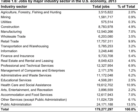
Table 1.6 provides the breakdown of jobs by industry in the U.S. Among the nation’s non-government industry sectors, the “Health Care and Social Assistance” sector is the largest employer, supporting 19.6 million jobs or 10.9% of total employment. The second largest employer is the “Retail Trade” sector, supporting 17.8 million jobs or 9.9% of the nation’s total employment. Altogether, the U.S. economy supports 179.3 million jobs.6

Table 1.6: Jobs by major industry sector in the U.S. economy, 2013

Industry sector Total jobs % of Total

Agriculture, Forestry, Fishing and Hunting 3,515,822 2.0%

Mining 1,581,717 0.9%

Utilities 575,514 0.3%

Construction 8,783,978 4.9% Manufacturing 12,540,266 7.0% Wholesale Trade 6,203,080 3.5% Retail Trade 17,757,311 9.9% Transportation and Warehousing 5,785,253 3.2% Information 3,248,446 1.8% Finance and Insurance 9,733,708 5.4% Real Estate and Rental and Leasing 8,049,423 4.5% Professional and Technical Services 12,327,954 6.9% Management of Companies and Enterprises 2,171,376 1.2% Administrative and Waste Services 11,172,048 6.2% Educational Services 4,508,281 2.5% Health Care and Social Assistance 19,612,702 10.9% Arts, Entertainment, and Recreation 3,896,559 2.2% Accommodation and Food Services 12,617,943 7.0% Other Services (except Public Administration) 11,024,729 6.1% Public Administration 24,171,188 13.5%

Total 179,277,297 100.0%

* Data reflect the most recent year for which data are available. EMSI data are updated quarterly.

┼_{Numbers may not add due to rounding.}

Source: EMSI complete employment data. 1.3.3 Earnings by education level

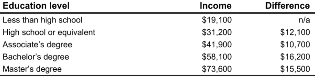
Table 1.7 and Figure 1.1 present mean income by education level at the midpoint of the average-aged worker’s career. These numbers are derived from EMSI’s complete employment data on

6_{Job numbers reflect EMSI’s complete employment data, which includes the following four job classes: 1) employees}

that are counted in the Bureau of Labor Statistics’ Quarterly Census of Employment and Wages (QCEW), 2) employees that are not covered by the federal or state unemployment insurance (UI) system and are thus excluded from QCEW, 3) self-employed workers, and 4) extended proprietors.

(15)

average income per worker in the nation.7_{As shown, students who achieve an associate’s degree can}

expect $41,900 in income per year, approximately $10,700 more than someone with a high school diploma. The difference between a high school diploma and the attainment of a bachelor’s degree is even greater – up to $26,900 in higher income.

Table 1.7: Expected income at the midpoint of individual's working career by education level

Education level Income Difference

Less than high school $19,100 n/a High school or equivalent $31,200 $12,100 Associate’s degree $41,900 $10,700 Bachelor’s degree $58,100 $16,200 Master’s degree $73,600 $15,500

Source: EMSI complete employment data.

Figure 1.1: Expected income by education level at career midpoint

$0 $10,000 $20,000 $30,000 $40,000 $50,000 $60,000 $70,000 $80,000

< HS HS Associate's Bachelor's Master's

1.4 Conclusion

This chapter presents the broader elements of the database used to determine the results of the study. Additional detail on data sources, assumptions, and general methods underlying the analyses are conveyed in the remaining chapters and appendices. The core of the findings is presented in the next two chapters – Chapter 2 considers the impact of community colleges on the national economy, and Chapter 3 looks at community colleges as an investment. The appendices detail a collection of miscellaneous theory and data issues.

7_{Wage rates in the EMSI SAM model combine state and federal sources to provide earnings that reflect complete}

employment in the nation, including proprietors, self-employed workers, and others not typically included in federal and state data, as well as benefits and all forms of employer contributions. As such, EMSI industry earnings-per-worker numbers are generally higher than those reported by other sources.

(16)

Chapter 2: Economic Impact Analysis

America’s community colleges impact the national economy in a variety of ways. The colleges are employers and buyers of goods and services. They attract monies to the U.S. that would not have otherwise entered the national economy through the expenditures of international students. Further, as primary sources of education to U.S. residents, community colleges supply trained workers to business and industry and contribute to associated increases in national output.

In this chapter we track the economic impact of America’s community colleges under three headings: 1) the impact of the colleges’ provision to international students; 2) the impact of international student living expenses, and 3) the impact of student productivity, comprising the added income created in the U.S. as former students expand the economy’s stock of human capital.

2.1 Impact of college provision to international students

Community colleges are just like other businesses in that they employ people and make purchases for supplies and services. Faculty and staff payroll counts as part of total income in the colleges’ respective service regions, and the spending of faculty and staff for groceries, apparel, and other household expenditures helps support local businesses. Community colleges are themselves purchasers of supplies and services, further supporting local vendors. Of course, some of the monies that colleges receive and spend in their service regions originally come from local sources, so the gross impact of college operations must be adjusted to account for these monies. Nonetheless, the net impact of colleges at the regional level is generally strongly positive, depending on the amount that colleges attract from outside their service regions and the extent to which they spend those monies locally.

At the national level, the situation is different. Nearly all of the colleges’ funding comes from sources within the U.S., which means the impacts of the colleges’ payroll and purchases do not inject new monies into the national economy. Rather, they simply represent a re-circulation of U.S. dollars. For this reason, the impact of college operations at the national level is necessarily assumed to be zero. The one notable exception is the amount collected by community colleges from international students for tuition and fees and for books and supplies. These are monies that would not have otherwise entered the U.S. economy if the community colleges did not exist. Once colleges receive these monies, they use them in the same way as they would use any other monies, i.e., by paying a portion of them to their employees and using the rest to help cover their operating expenses. These expenditures then create a ripple effect that generates still more jobs and income throughout the economy.

Recognizing that the national impact of college operations is limited to the extent to which the colleges attract monies from outside the U.S., this section focuses strictly on the impact of the colleges’ spending of the monies they collect from international students. In 2012, approximately

(17)

146,500 international students attended America’s community colleges and paid an estimated $1.2 billion to the colleges for tuition and fees and books and supplies. Assuming that the colleges spent these monies proportionately to the breakdown of college spending in Table 1.3, approximately $684.1 million (or 57%) of the monies collected from international students was used to cover the colleges’ payroll, and the remaining $513.5 million (or 43%) was used to cover the colleges’ capital depreciation and other operating expenses.

Table 2.1 presents the impacts. The top row shows the overall labor and non-labor income in the U.S., which we use as the backdrop for gauging the relative role of the colleges in the national economy. These data are the same as the total labor and non-labor income figures provided in Table 1.5 of Chapter 1.

Table 2.1: Impact of college provision to international students

Labor income (thousands)

Non-labor income (thousands)

Total income (thousands)

% of total income in nation

Total income in nation $9,254,082,495 $5,831,514,342 $15,085,596,837 100.0%

Initial effect $684,105 $0 $684,105 <0.1%

Multiplier effect

Direct effect $281,504 $274,422 $555,926 <0.1% Indirect effect $169,288 $128,324 $297,611 <0.1%

Total multiplier effect $450,791 $402,746 $853,537 <0.1% Total effect (initial + multiplier) $1,134,897 $402,746 $1,537,643 <0.1%

Source: EMSI SAM model.

As for the impacts themselves, we follow best practice and draw the distinction between initial effects and multiplier effects. The initial effect is simple – it amounts to the $684.1 million used by the colleges to help cover employee payroll. Note that, as public entities, community colleges do not generate property income in the traditional sense, so non-labor income is not associated with college operations under the initial effect.

Multiplier effects refer to the additional income created in the economy as the colleges and their employees spend money. They are categorized according to the following two effects: the direct effect and the indirect effect. Direct effects refer to the income created by the industries initially affected by the spending of the colleges and their employees. Indirect effects occur as the supply chain of the initial industries creates even more income.8

Calculating multiplier effects requires a specialized Social Accounting Matrix (SAM) model that captures the interconnection of industries, government, and households in the U.S. The EMSI SAM model contains approximately 1,100 industry sectors at the highest level of detail available in the North American Industry Classification System (NAICS), and it supplies the industry-specific

8_{Many regional studies also include so-called “induced effects” created by consumer spending. In national models,}

(18)

multipliers required to determine the impacts associated with economic activity. For more information on the EMSI SAM model and its data sources, see Appendix 3.

The first step in estimating the multiplier effect is to map the colleges’ payroll and expenses to the approximately 1,100 industry sectors of the EMSI SAM model. Assuming that the spending patterns of college personnel approximately match those of the average consumer, we map the $684.1 million in college payroll to spending on industry outputs using national household expenditure coefficients supplied by EMSI’s national SAM. For the other two expenditure categories (i.e., capital depreciation and all other expenditures), we again assume that the colleges’ spending patterns approximately match national averages and apply the national spending coefficients for NAICS 611210 (Junior Colleges).9 Capital depreciation is mapped to the construction sectors of NAICS 611210 and the colleges’ remaining expenditures to the non-construction sectors of NAICS 611210.

We now have three vectors detailing the spending of the monies collected by community colleges from international students: one for college payroll, another for capital items, and a third for the colleges’ purchases of supplies and services. These are entered into the SAM model’s multiplier matrix, which in turn provides an estimate of the associated multiplier effects on national sales. We convert the sales figures to income using income-to-sales ratios, also provided by the SAM model. Final results appear in the section labeled “Multiplier effect” in Table 2.1. Altogether, the payroll and expenses spent by the colleges to support their provision to international students creates $450.8 million in labor income and another $402.7 million in non-labor income through multiplier effects – a total of $853.5 million. Adding the $853.5 million in direct and indirect multiplier effects to the $684.1 million in initial effects generates a total of $1.5 billion in impacts.

2.2 Impact of international student living expenses

In addition to the monies they spend on tuition and fees and on books and supplies, international students also spend money at U.S. businesses to purchase groceries, rent accommodation, pay for transportation, and so on. These expenses supported American jobs and created new income in the national economy. The average living expenses of international students appear in the first section of Table 2.2, equal to $8,390 per student. Multiplying the $8,390 in annual costs by the number of international students generates gross sales of $1.2 billion.

(19)

Table 2.2: Average student cost of attendance and total sales generated by international students, 2012

Room and board $5,546 Personal expenses $1,612 Transportation $1,232

Total expenses per student (A) $8,390

Number of international students (B) 146,472 Gross sales generated by international students (A * B) $1,228,874,038

Source: Data on the cost of attendance and the number of international students supplied by IPEDS.

Estimating the impacts generated by the $1.2 billion in international student living expenses follows a procedure similar to described in the previous section. We begin by mapping the $1.2 billion in sales to the industry sectors in the SAM model and then run the net sales figures through the SAM model to derive multiplier effects. Finally, we convert the results to income through the application of income-to-sales ratios.

Table 2.3 presents the results. The initial effect is $0 because the impact of international students only occurs when they spend part of their income to make a purchase. Otherwise, the students’ income has no impact on the national economy. The impact of international student spending thus falls entirely under the multiplier effect, equal to a total of $1.1 billion in added income. This value represents the direct added income created at the businesses patronized by the students and the indirect added income created by the supply chain of those businesses.

Table 2.3: Impact of international student living expenses

Initial effect $0 $0 $0 <0.1%

Multiplier effect

Direct effect $357,189 $367,823 $725,012 <0.1% Indirect effect $182,116 $155,547 $337,663 <0.1%

Total multiplier effect $539,305 $523,370 $1,062,675 <0.1% Total effect (initial + multiplier) $539,305 $523,370 $1,062,675 <0.1%

2.3 Impact of student productivity

The greatest economic impact of America’s community colleges stems from the education, skills training, and career enhancement that they provide. Since they were established, the colleges have supplied skills training to students who have subsequently entered or re-entered the U.S. workforce. As these skills accumulated, the nation’s stock of human capital expanded, boosting the competiveness of existing industries, attracting new industries, and generally enlarging overall

(20)

output. The sum of all these several and varied effects, measured in terms of added national income, constitutes the total impact of current and past student productivity on the national economy. The student productivity effect differs from the effect of international students in one fundamental way. Whereas international student spending depends on an annually-renewed injection of new sales in the national economy, the student productivity effect is the result of years of past instruction and the associated workforce accumulation of college skills. Should America’s community colleges cease to exist, international students would no longer come to the U.S. to attend the colleges and the effect of their spending for tuition and fees, books and supplies, and living expenses would also immediately cease to exist; however, the impact of the colleges’ former students would continue, as long as those students remained active in the workforce. Over time, though, students would leave the workforce, and the expanded economic output that they provide through their increased productivity would leave with them.

The initial effect of student productivity comprises two main components. The first and largest of these is the added labor income (i.e., higher wages) of former students. Higher wages occur as the increased productivity of workers leads to greater business output. The reward to increased productivity does not stop there, however. Skilled workers make capital goods (e.g., buildings, production facilities, equipment, etc.) more productive too, thereby increasing the return on capital in the form of higher profits. The second component of the initial effect thus comprises the added non-labor income (i.e., higher profits) of the businesses that employ the students.

The first step in estimating the initial effect of student productivity is to determine the added labor income stemming from the students’ higher wages. We begin by assembling the record of historical student headcounts at the colleges over the past 30 years,10_{from 1983 to 2012. From this vector of}

historical enrollments we remove the number of students who are not currently active in the workforce, whether because they’re still enrolled in education, or because they’re unemployed, or because they’re out of the workforce completely due to retirement or death. We estimate the historical employment patterns of students using the following sets of data or assumptions: 1) a set of settling-in factors to determine how long it takes the average student to settle into a career;11 2) death rates from the National Center for Health Statistics; (3) retirement rates from the Social Security Administration; and (4) unemployment rates from the Bureau of Labor Statistics. The end

10_{We apply a 30-year time horizon because the data on students who attended college prior to 1983 is less reliable, and}

because most of the students whom the colleges served more than 30 years ago had left the workforce by 2012. Historical enrollment data for the years 2002 to 2012 come from IPEDS. The EMSI college impact model projects the historical enrollments backwards for the remaining years using the average annual change in enrollment indicated in the observed data.

11_{Settling-in factors are used to delay the onset of the benefits to students in order to allow time for them to find}

employment and settle into their careers. In the absence of hard data, we assume a range between one and three years for students who graduate with a certificate or a degree, and between zero and five years for students who do not receive an award.

(21)

result of these several computations is an estimate of the portion of students who were still actively employed as of 2012.

The next step is to transition from the number of students who were still employed to the number of skills they acquired from America’s community colleges.12_{The students’ production of credit}

hours serves as a reasonable proxy for accumulated skills. Table 1.4 in Chapter 1 provides the average number of credit hours completed per student in 2012, equal to 14.0 credit hours. Using historical credit production from IPEDS, we can also derive the average number of credit hours per student for previous years.13_{The total number of credit hours for all years in the time horizon – 3.1}

billion – appears in the top row of Table 2.4.

Table 2.4: Number of credit hours in workforce and initial labor income created in national economy

Number of credit hours in workforce 3,135,726,517 Average value per credit hour $174

Initial labor income, gross $545,905,812,469

Percent reduction for alternative education opportunities 23%

Initial labor income, net $421,116,435,761

Source: EMSI college impact model.

The next row in Table 2.4 shows the average value per credit hour, equal to $174. This value represents the average increase in wages that former students received during the analysis year for every credit hour they completed at the colleges. The value per credit hour varies depending on the students’ age, with the highest value applied to the credit hour production of students who had been employed the longest by 2012, and the lowest value per credit hour applied to students who were just entering the workforce. More information on the theory and calculations behind the value per credit hour appears in Appendix 4. In determining the amount of added labor income attributable to former students, we multiply the credit hour production of former students in each year of the historical time horizon times the corresponding average value per credit hour for that year, then sum the products together. This calculation yields approximately $545.9 billion in gross labor income in increased wages received by former students in 2012 (as shown in Table 2.4).

The next row in the table shows an adjustment that we make to account for counterfactual outcomes. As discussed above, counterfactual outcomes in economic analysis represent what would have happened if a given event had not occurred. The event in this case is the training provided by

12_{Students who enroll at the colleges for more than one year were counted at least twice, if not more, in the historical}

enrollment data. However, credit hours remain distinct regardless of when and by whom they were earned, so there is no duplication in the credit hour counts. In calculating the impact of student productivity, it is the number of credit hours – not the number of enrollments – that drives the results. As such, the duplication in the enrollment data across years has no bearing on the study outcomes.

13_{As with the enrollment data, only about ten years’ worth of credit production data comes from IPEDs. Prior to that,}

the data become increasingly less reliable. For the missing years, the model assumes a constant ratio of credits to enrollments based on the weighted average number of credits per enrollee in the years for which data are available.

(22)

America’s community colleges and subsequent influx of skilled labor into the national economy. Our assumption is that, if a portion of the students could have received training even if the community colleges did not exist, the higher wages that accrue to those students cannot be counted as added labor income in the nation. The adjustment for alternative education opportunities amounts to a 23% reduction of the $545.9 billion in added labor income, meaning that 23% of the added labor income would have been generated in the U.S. anyway, even if the colleges did not exist. For more information on the calculation of the alternative education variable, see Appendix 5. The $421.1 billion in added labor income appears under the initial effect in the “Labor income” column of Table 2.5. To this we add an estimate for initial non-labor income. As discussed earlier in this section, businesses that employ former students of America’s community colleges see higher profits as a result of the increased productivity of their capital assets. To estimate this additional income, we allocate the initial increase in labor income ($421.1 billion) to the specific NAICS six-digit industry sectors where former students are employed. This allocation entails a process that maps completers14_{to the detailed occupations for which those completers have been trained, and}

then maps the detailed occupations to the six-digit industry sectors in the national SAM model. Completer data comes from the Integrated Postsecondary Education Data System (IPEDS), which organizes program completions by institution according to the Classification of Instructional Programs (CIP) developed by the National Center for Education Statistics (NCES). Using a crosswalk created by NCES and the Bureau of Labor Statistics (BLS), we map the breakdown of completers by CIP code to the approximately 700 detailed occupations in the Standard Occupational Classification (SOC) system used by the BLS. We then allocate the $421.1 billion in initial labor income effects proportionately to the SOC framework based on the occupational distribution of the completions. Finally, we apply a matrix of wages by industry and by occupation from the national SAM model to map the detailed occupational distribution of the $421.1 billion to the NAICS six-digit industry sectors of the model.15

Once these allocations are complete, we apply the ratio of non-labor to labor income provided by the SAM model for each sector to our estimate of initial labor income. This computation yields an estimated $119.2 billion in non-labor income attributable to the former students. Summing initial labor and non-labor income together provides the total initial effect of student productivity in the national economy, equal to approximately $540.4 billion.

14_{IPEDS defines a completer as the following: “A student who receives a degree, diploma, certificate, or other formal}

award. In order to be considered a completer, the degree/award must actually be conferred.” IPEDS Glossary, accessed July 2013, http://nces.ed.gov/ipeds/glossary/?text=1.

15_{For example, if the SAM model indicates that 20% of wages paid to workers in SOC 51-4121 (Welders) occur in}

NAICS 332313 (Plate Work Manufacturing), then we allocate 20% of the initial labor income effect under SOC 51-4121 to NAICS 332313.

(23)

Table 2.5: Impact of student productivity

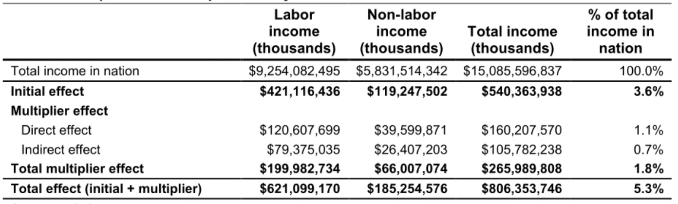
Initial effect $421,116,436 $119,247,502 $540,363,938 3.6% Multiplier effect

Direct effect $120,607,699 $39,599,871 $160,207,570 1.1% Indirect effect $79,375,035 $26,407,203 $105,782,238 0.7%

Total multiplier effect $199,982,734 $66,007,074 $265,989,808 1.8% Total effect (initial + multiplier) $621,099,170 $185,254,576 $806,353,746 5.3%

The next few rows of Table 2.5 show the multiplier effects of student productivity. Multiplier effects occur as students generate an increased demand for consumer goods and services through the expenditure of their higher wages. Further, as the industries where students of America’s community colleges are employed increase their output, there is a corresponding increase in the demand for input from the industries in the employers’ supply chain. Together, the incomes generated by the expansions in business input purchases and household spending constitute the multiplier effect of the increased productivity of former students.

To estimate multiplier effects, we convert the industry-specific income figures generated through the initial effect to sales using sales-to-income ratios from the SAM model. We then run the values through the SAM’s multiplier matrix to determine the corresponding increases in industry output that occur in the nation. Finally, we convert all increases in sales back to income using the income-to-sales ratios supplied by the SAM model. The final results are $200 billion in labor income and $66 billion in non-labor income, for an overall total of $266 billion in multiplier effects. The grand total impact of student productivity thus comes to $806.4 billion, the sum of all initial and multiplier labor and non-labor income effects. The total figures appear in the last row of Table 2.5.

2.4 Summary of impacts

Table 2.6 displays the grand total impact of America’s community colleges on the national economy in 2012, including the impact of the colleges’ provision to international students, the impact of international student living expenses, and the impact of student productivity.

(24)

Table 2.6: Total effect, 2011-12

Total

(thousands) % of Total

Total income in nation $15,085,596,837 100.0%

Impact of international students

Impact of college provision to international students $1,537,643 <0.1% Impact of international student living expenses $1,062,675 <0.1%

Impact of student productivity $806,353,746 5.3%

Total $808,954,064 5.4%

Source: EMSI college impact model.

These results demonstrate several important points. First, community colleges create economic impacts through the monies they spend to support their international students, through the living expenses of their international students, and through the increase in productivity as their former students remain active in the U.S. workforce. Second, the student productivity effect is by far the largest and most important impact of America’s community colleges, stemming from higher incomes of students and their employers. And third, income in the U.S. would be substantially lower without the educational activities of America’s community colleges.

Calculating Job Equivalents Based on Income

In this study the impacts of America’s community colleges on the national economy are expressed in terms of income, specifically, the added income that would not have occurred in the nation if the colleges did not exist. Added income means that there is more money to spend, and increased spending means an increased demand for goods and services. Businesses hire more people to meet this demand, and thus jobs are created.

Not every job is the same, however. Some jobs pay more, others less. Some are full-time, others are part-time. Some jobs are year-round, others are temporary. Deciding what constitutes an actual job, therefore, is difficult to do. To address this problem, this study counts all jobs equally and reports them in terms of job equivalents, i.e., the number of average-wage jobs that a given amount of income could potentially support. Job equivalents are calculated by dividing the added income created by the colleges and their students by the average income per worker in the U.S. Based on the added income figures from Table 2.6, the overall income created by America’s community colleges during the analysis year supported 15.5 million average-wage jobs in the U.S. economy.

(25)

Chapter 3: Investment Analysis

Investment analysis is the process of evaluating total costs and measuring these against total benefits to determine whether or not a proposed venture will be profitable. If benefits outweigh costs, then the investment is worthwhile. If costs outweigh benefits, then the investment will lose money and is thus considered infeasible. In this chapter, we consider America’s community colleges as an investment from the perspectives of students, society, and taxpayers.

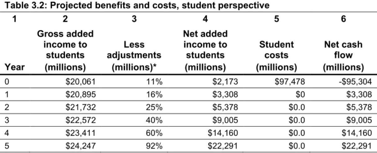
3.1 Student perspective

Analyzing the benefits and costs of education from the perspective of students is the most obvious – they give up time and money to go to college in return for a lifetime of higher income. The cost component of the analysis thus comprises the monies students pay (in the form of tuition and fees and forgone time and money), and the benefit component focuses on the extent to which the students’ incomes increase as a result of their education.

3.1.1 Calculating student costs

Student costs consist of two main items: direct outlays and opportunity costs. Direct outlays include tuition and fees, equal to $10.2 billion from Table 1.2. Students also must pay for the cost of books and supplies. On average, full-time students spent $1,400 each on books and supplies during the reporting year.16 Multiplying this figure times the number of full-time equivalents (FTEs) produced by America’s community college students in 201217_{generates a total cost of $7.6 billion for books}

and supplies.

Another component of the students’ direct outlays is the interest they pay on loans. According to the National Postsecondary Student Aid Study (NPSAS), 17.6% of undergraduate students attending public two-year colleges in 2011-12 received loans at an average amount of $4,700 per student.18

Assuming that students pay off these loans within a ten-year period at an interest rate of 5.83%, the present value of the interest comes to $882.7 million.19

16_{Based on the data supplied by IPEDS.}

17_{A single FTE is equal to 30 credit hours, so there were 5.4 million FTEs produced by America’s community college}

students, equal to 163 million credit hours divided by 30.

18_{David Radwin, et al, 2}_{011-12 National Postsecondary Student Aid Study (NPSAS:12): Student Financial Aid Estimates for}

2011-12, NCES 2013-165, Institute of Education Sciences, U.S. Department of Education (Washington, DC, National

Center for Education Statistics, August 2013).

19_{The fixed interest rate on direct subsidized and unsubsidized loans for undergraduate students is 3.86% (see Federal}

Student Aid, “Loan Interest Rates by Disbursement Dates,” Interest Rates and Fees, accessed December 2013, http://studentaid.ed.gov/types/loans/interest-rates). The Consumer Financial Protection Bureau reports that the average interest rate on private student loans is 7.8% (see Consumer Financial Protection Bureau, “Private Student Loans," August 2012. The 5.83% interest rate used in this study is an average of public and private interest rates. This

(26)

Opportunity cost is the most difficult component of student costs to estimate. It measures the value of time and earnings forgone by students who go to college rather than work. To calculate it, we need to know the difference between the students’ full earning potential and what they actually earn while attending college.

We derive the students’ full earning potential by weighting the average annual income levels in Table 1.7 according to the education level breakdown of the student population when they first enrolled.20

However, the income levels in Table 1.7 reflect what average workers earn at the midpoint of their careers, not while attending college. Because of this, we adjust the income levels to the average age of the student population (23) to better reflect their wages at their current age.21_{This calculation}

yields an average full earning potential of $21,598 per student.

In determining what students earn while attending college, an important factor to consider is the time that they actually spend at college, since this is the only time that they are required to give up a portion of their earnings. We use the students’ credit hour production as a proxy for time, under the assumption that the more credit hours students earn, the less time they have to work, and, consequently, the greater their forgone earnings. Overall, students at America’s community colleges earned an average of 14.0 credit hours per student, which is approximately equal to 47% of a full academic year.22 We thus include no more than $10,104 (or 47%) of the students’ full earning potential in the opportunity cost calculations.

Another factor to consider is the students’ employment status while attending college. An estimated 81% of students attending America’s community colleges are employed.23 For the 19% that are not working, we assume that they are either seeking work or planning to seek work once they complete their educational goals. By choosing to go to college, therefore, non-working students give up everything that they can potentially earn during the academic year (i.e., the $10,104). The total value of their forgone income thus comes to $21.8 billion.

Working students are able to maintain all or part of their income while enrolled. However, many of them hold jobs that pay less than statistical averages, usually because those are the only jobs they can find that accommodate their course schedule. These jobs tend to be at entry level, such as restaurant servers or cashiers. To account for this, we assume that working students hold jobs that pay 58% of

estimate is probably on the high side given that students are more likely to take out public loans, which tend to have lower interest rates than private loans.

20_{The students’ level of education at entry is estimated based on data supplied by EMSI’s sample colleges.}

21_{We use the lifecycle earnings function identified by Jacob Mincer to scale the income levels to the students’ current}

age. See Jacob Mincer, “Investment in Human Capital and Personal Income Distribution,” Journal of Political Economy, vol. 66 issue 4, August 1958: 281-302. Further discussion on the Mincer function and its role in calculating the students’ return on investment appears later in this chapter and in Appendix 4.

22_{Equal to 14.0 credit hours divided by 30, the assumed number of credit hours in a full-time academic year.} 23_{National Center for Education Statistics, “Profile of Undergraduate Students: 2007-08,” NCES, September 2010.}

(27)

what they would have earned had they chosen to work full-time rather than go to college.24_The

remaining 42% comprises the percent of their full earning potential that they forgo. Obviously this assumption varies by person – some students forego more and others less. Without knowing the actual jobs that students hold while attending, however, the 42% in forgone earnings serves as a reasonable average.

Working students also give up a portion of their leisure time in order to go to school, and mainstream theory places a value on this.25 According to the Bureau of Labor Statistics American Time Use Survey, students forgo up to 1.4 hours of leisure time per day.26_{Assuming that an hour of}

leisure is equal in value to an hour of work, we derive the total cost of leisure by multiplying the number of leisure hours foregone during the academic year by the average hourly pay of the students’ full earning potential. For working students, therefore, their total opportunity cost comes to $56.9 billion, equal to the sum of their foregone income ($40.5 billion) and forgone leisure time ($16.4 billion).

The steps leading up to the calculation of student costs appear in Table 3.1. Direct outlays amount to $18.7 billion, the sum of tuition and fees ($10.2 billion) and books and supplies ($7.6 billion). Opportunity costs for working and non-working students amount to $78.7 billion. Summing all values together yields a total of $97.5 billion in student costs.

Table 3.1: Student costs, 2012 (thousands)

Direct outlays

Tuition and fees $10,237,818 Books and supplies $7,609,225 Present value of interest on loans $882,741

Total direct outlays $18,729,783

Opportunity costs

Earnings forgone by non-working students $21,827,265 Earnings forgone by working students $40,502,015 Value of leisure time forgone by working students $16,418,483

Total opportunity costs $78,747,764

Total student costs $97,477,546

Source: Based on data supplied by IPEDS, EMSI’s sample colleges, and outputs of the EMSI college impact model.

24_{The 58% assumption is based on the average hourly wage of the jobs most commonly held by working students}

divided by the national average hourly wage. Occupational wage estimates are published by the Bureau of Labor Statistics (see http://www.bls.gov/oes/current/oes_nat.htm).

25_{See James M. Henderson and Richard E. Quandt,}_{Microeconomic Theory: A Mathematical Approach}_{(New York:}

McGraw-Hill Book Company, 1971).

26_{“Charts by Topic: Leisure and sports activities,” Bureau of Labor Statistics American Time Use Survey, last modified}