Vol 8, No 2 (2016)

(1)

International Journal of Communication Networks and Information Security (IJCNIS) Vol. 8, No. 2, August 2016

Smart Algorithms for Hierarchical Clustering in

Optical Network

Shadi Atalla

1

, Saed Tarapiah

2

, Mahmoud El Hendy

1

and Kamarul Faizal Bin Hashim

1

College of Engineering and Information Technology (CEIT), University of Dubai, Dubai, UAE 2 _{Telecommunication Engineering Department, An-Najah National University, Nablus, Palestine}

[email protected], [email protected], [email protected] and [email protected]

Abstract: Network design process is a very important in order to

balance between the investment in the network and the supervises offered to the network user, taking into consideration, both minimizing the network investment cost, on the other hand, maximizing the quality of service offered to the customers as well. Partitioning the network to smaller sub-networks called clusters is required during the design process in order to ease studying the whole network and achieve the design process as a trade-off between several attributes such as quality of service, reliability, cost, and management. Under Clustered Architecture for Nodes in an Optical Network (CANON), a large scale optical network is partitioned into a number of geographically limited areas taking into account many different criteria like administrative domains, topological characteristics, traffic patterns, legacy infrastructure etc. An important consideration is that each of these clusters is comprised of a group of nodes in geographical proximity. The clusters can coincide with administrative domains but there could be many cases where two or more clusters belong to the same administrative domain. Therefore, in the most general case the partitioning into specific clusters can be either an off-line or an on-line process. In this work only the off-on-line case is considered. In this Study, we look at the problem of designing efficient 2-level Hierarchical Optical Networks (HON), in the context of network costs optimization. 2-level HON paradigm only has local rings to connect disjoint sets of nodes and a global sub-mesh to interconnect all the local rings. We present a Hierarchical algorithm that is based on two phases. We present results for scenarios containing a set of real optical topologies.

Keywords: Optical Networks, Clustering, Algorithms.

1. Introduction

With the rapid development of wavelength division multiplexing (WDM) technology, optical networks could employ hundreds of wavelengths to support increasing traffic. In such dynamically re-configurable networks, routing and add-drop are performed for each individual wavelength in every node, thus resulting in increased complexity as well as capital and operational expenditures [1, 2]. Optical networks are evolving into a complex interconnection of circuit switched domains and layers (or granularities), with the border of domains being driven by many factors. Moreover, that in existing networks resources are typically managed and controlled in a hierarchical manner. With the increase in the number of entities that need to be controlled within a hierarchical framework in optical networks. The hierarchical design process of Core networks has to balance the investment in the network against the QoS and the benefits provided to the network users.

Usually this process involves the partition of the network into smaller disjoint sub-networks (Clusters) in order to reach a good trade-off between several agents such as cost, management, reliability and quality of service.

In this study we considered a new Core network architecture know as CANON, where a large scale network is partitioned into a number of clusters taking into account various criteria like administrative domains, topological characteristics, traffic patterns, legacy infrastructure etc.

An important consideration is that each of these clusters is comprised of a group of nodes in geographical proximity. The clusters can coincide with administrative domains but there could be many cases where two or more clusters belong to the same administrative domain.

In the CANON architecture, the network is a buildup of a number of clusters. Routing is hierarchical:

• The intra-cluster routing transfers all the traffic within the same cluster according to a ring logical topology. One aggregation node denoted as Core Transit Node (CTN). Similarly, the CTN aggregates also all the traffic coming from different clusters and directed to its cluster.

• The inter-cluster routing transfers all the traffic among different clusters according to a generic mesh logical topology among all CTNs.

In this study, we propose a new hierarchical approach that partitions a general mesh optical network into a number of clusters that are compatible with the CANON paradigm. These clusters are built in a way that minimizes network resources required to sustain some given traffic demand based on CANON hierarchical routing.

(2)

This study illustrates several design parameters that needed to be considered in determining the network cost while varying a number of clusters and placement of CTNs in the network. Mainly the network costs which are considered by this study are:

• The count of the optical switching ports; we would use the minimum possible number of optical switching ports to support the given traffic.

• wavelengths, at the same time, we would also like to use the minimum possible number of wavelengths since using more wavelengths incurs additional equipment cost in the optical layer,

• Hops, this parameter refers to the maximum number of hops taken up by a light path. The reason this parameter becomes important is that it becomes more difficult to design the transmission system as the number of hops increases, which again increases the cost of optical layer equipment.

In general, we will see that there is a trade-off between these different parameters. Though, in this work only the off-line case is considered, as this work focuses on topology design phase which can be considered as static solution which lasts for very long time. This assumption gives the researchers the time required for running the proposed algorithms to find an optimal design solution. In the meanwhile, online case is more important for handling frequent changes in the networks parameters such as the offered network traffic Matrix where new solutions are always demanded in short time frame where this time budget is not enough to find an optimal design solution and where simple heuristics cloud be proposed to find an acceptable solutions in fast times.

2. Hierarchical Clustering

We consider an optical network with N nodes, connected by links that consist of one fiber per direction, each of them carrying W wavelengths.

2.1. Optimal partition and routing problem

The design objective is to sustain some given traffic demand over a network based on CANON paradigm while minimizing the total number of optical ports and the number of wavelengths in the whole network.

This optimization problem implies to solve the two classical problems of Logical Topology Design (LTD) and Routing and Wavelength Assignment (RWA). The LTD is based on the following phases:

1) network partition, in which the network is partitioned into K clusters;

2) logical ring selection for each cluster, in which a logical ring is determined among all the nodes in the same cluster;

3) CTN selection for each cluster, in which one node is designated as CTN.

4) Logical mesh selection among the CTNs, finding a set of light paths among all the CTNs in the network.

In the RWA, the traffic demand is routed on the physical topology. Here, each one of the logical rings and the light paths is assigned a path on the underlying physical topology of the original mesh network. The traffic is routed according to the hierarchical intra-cluster and inter-cluster routing described above. Where we presented a hierarchical Optical Network Clustering algorithm consists of two phases.

• Logical Topology design

i. Clustering. Partition the network into K clusters, then identify logical rings inside the clusters. ii. CTN selection. Designate one node in each

cluster as the CTN, then find a set of light paths for communications between all the CTNs in the network.

• Routing And wavelength Assignment

i. On the physical topology. Each one of the logical rings and the light paths is assigned a path on the underlying physical topology of the original mesh network. Traffic routing.

This phase is further subdivided into two parts: intracluster traffic routing. Intercluster traffic routing.

We impose that the intra-cluster traffic flows in only one direction around the ring, a common situation because of protection requirements. However, our methods can be easily extended to bidirectional rings. Note that the intra-cluster ring has been chosen for its well-known advantages in terms of dimensioning, management, multicast, protection and restoration, etc. This also constitutes a natural migration step when starting from today's SDH rings. A new algorithm - for clustering optical Core network into smaller sub-networks- has been proposed in order to reach a good trade-off between several agents, such as cost and performance. We have carried out a thorough study and simulation about the use of our clustering algorithm on a set of real optical Core networks.

2.2. System model

The network physical topology is described by an undirected graph G = (V, E), where V is set of N nodes and E is a set of links. Let ejl be the link between vj ∈ V and vl∈ V and c (ejl)

its physical distance (i.e., expressed in kilometers). Let E (vj)

be the set of links connected to vj.

Let Ci⊆ V be the i-th cluster and ni = |Ci| be the number of

nodes in Ci. Within each cluster Ci, the unidirectional logical

ring LRi interconnects the ni nodes; LRi(j), with

j = 1. . . ni, is the j-the node in LRi (starting from some

arbitrary node in the cluster). Similarly, the physical ring PRi

is a cycle that contains all the nodes of the physical topology needed to construct the corresponding LRi. An inter-cluster

mesh connects the K CTNs. Let CTNi denote the CTN node of

cluster Ci. The routing among the CTNs is the shortest path,

according to the physical distance.

2.3. Toy example

Consider the example of LTD and RWA shown in Figure. 1. The original physical network with N = 12 nodes is shown in Figure. 1(a) where circles represent the optical nodes and lines is the fiber links. Assume K = 3. Initially, as shown in Figure. 1(b), the network is partitioned into three clusters C 1

, C 2 , and C 3 , where C 1 = {1, 2, 8, 9}, C 2 = {7, 6, 10, 11},

and C 3 = {3, 4, 5, 12}. Figure. 1(c) shows the CTNs selected

in each cluster, where the CTNs have been represented by the rectangle. Figure. 1(d) shows the unidirectional logical ring

LR within each cluster. The nodes inside C 1 are

interconnected by LR 1 = (2, 1, 8, 9), similarly LR 2 = (7, 6,

10, 11) and LR3 = (4, 3, 12, 5). Figure. 1(e) shows the

physical rings corresponding to the intra-cluster rings: PR1

= (2, 1, 8, 9, 10, 7), PR2 = (6, 7, 10, 11) and PR3 = (3, 6, 11,

(3)

Figure 1. Example

of LTD and RWA for K = 3 and N = 12

2.4. Traffic demand

We define the traffic demand matrix T = [t(s, d)], where t(s,d) denotes the traffic demand, measured in integer multiples of the wavelength capacity, to be carried from node s to node d. Given the network partition, we define a ni × ni

matrix Ti intra ,as the intra-cluster traffic matrix, where T i

intra(s,d) denotes the traffic volume to be exchanged among

nodes s,d Ci . For all the K clusters, we define the

inter-cluster traffic matrix Tinter of size k×k, where Tinter (Ci, Cj)

denotes the aggregated traffic exchanged between different clusters, i.e. routed through the corresponding CTNs.

3. Related Work

In general, network partitioning problem is a well-studied subject. Mathematically, the network partitioning is defined on a graph G (V, E), such that it is possible to partition G into smaller partitions with specific properties, while the input to the partitioning algorithms generally consist of a set of nodes and edge weights, while the output is a partition of the nodes that optimizes a given objective function. Methods of graph partitioning include bi-partitioning, balanced partitioning, partitioning with cost optimization, minimizing cut-size, and so on. Some clustering studies consider the traffic matrix only. As for optical networks, the authors in [1] proposed to partition nodes in a ring such that groups of nodes are exist that have a high amount of traffic to each other, but there is comparatively less traffic between nodes belonging to different such groups, as it is desirable for traffic demands within a cluster to be denser than inter-cluster traffic. The MTSP problem is NP-Complete [2], a heuristic based

solution is used to approximate the optimal one. Here, to perform network clustering: our options are the following i) based on the physical topology. ii) based on T. iii) distance traffic product solution. We have studied the i and ii.

3.1. Simulated Annealing

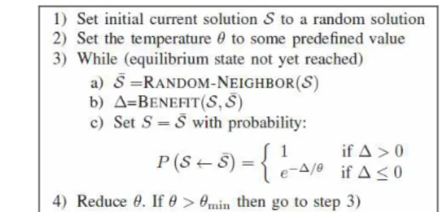
Simulated annealing (SA) is a generic probabilistic meta- heuristic for solving combinatorial problems [3]. SA is based on the analogy to physical annealing [4]. SA tries to find a good approximation to the global optimum of a given function in a large search space. So, it tries to avoid being trapped in local optima by accepting both ”good” and ”bad” moves, and gradually lowering the probability of accepting ”bad” moves. Even though in theory, SA can find the global optimum. For certain problems, SA is efficient if the goal is mere to find an acceptably good solution in a fixed amount of time, rather than the best possible solution. [5] [6] as typically implemented [3], SA approach involves a pair of nested loops and three additional parameters, cooling ratio r and two real numbers are the minimum and the maximum values of temperature θ.

Let us define the following: A solution S denotes a feasible solution for the problem. A neighbor solution S̄ is a new solution of the problem that is produced by altering S in some particular way. F (S) is the cost function that is being optimized by SA. Figure 2 depicts the SA algorithm. [Path, d] =Shortest-Path (G, v1, v2) is a function that determines

two outputs. The first is a path, which represents the minimum length path from node v1 to node v2 in G. The

second is d, which represents the physical distance of a path. We define Paths = [Paths (s, d)] that is N × N × N matrix, where Paths(s, d) is an array of nodes having the shortest path between node s and node d. Similarly, a distance matrix that is N × N matrix denoted as dist = [dist (s, d)], where dist (s, d) R+ denotes the shortest path between node s and node d according to the physical distance.

At the initialization step 1, it set S to a random feasible solution. After that, the algorithm executes two loops. An outer loop is shown by step 5 and the inner loop is depicted in step 4. The outer loop runs for a fixed number of iterations, this number is bounded by the initial and the final θ. The inner loop is nested and executed inside the outer loop. In each the inner loop iteration, the algorithm generates S̄ then it computes benefit of S̄ compared to S equals ∆ = F(S) − F (S̄) then the algorithm decides to mark the S̄ as the current solution or not based on the equation in shown in step 3.

Figure 2.

Simulated annealing structure of the problem used

in this work.

(4)

algorithm are not independent for each problem instance. We repeat the process until no permutation of the parameters can improve the performance.

3.2. ESA

So, we propose a new implementation based on Extended Simulated Annealing (ESA) algorithm described in [5]. ESA is used to solve the MTSP problem. Where distances between cities are computed by Euclidean distance. The ESA has a good performance in term of quality and running time. It was tested with a network of 400 cities, and the tests were performed on an IBM PC-586(400MHz). The tests take less than 51 minutes to output the results. Moreover, ESA can solve the MTSP without any transformation into a standard form, unlike most heuristic algorithms [7]. Hence, we need to solve MTSP problem with an input being the shortest-path not the Euclidean distance, modifications are needed to be introduced to ESA so it suits our problem. In fact, if we try to solve our problem using ESA, it could produce physical rings that traverse a node more than once.

4. LTD - Network partition

The number of clusters, their composition, the number of nodes within each cluster, and the corresponding CTNs must be selected in a way that helps to achieve the goal of minimizing the resources needed to carry the traffic demands. The selection of clusters is a complex and difficult task, as it depends on both the physical topology of the network and the traffic matrix. To illustrate this point, consider the tradeoffs involved in determining the number of clusters. If K is very small, the diameter and number of nodes of each cluster will likely be large. Hence, the optical light paths traverse long distances which lead to increase the number of wavelength in the whole network. Moreover a large amount of inter-cluster traffic will lead to bottlenecks at the CTNs. On the other hand, a large K value implies a small number of nodes within each cluster. In this case, the amount of intra-cluster traffic will be small, resulting underutilize the capacity of the light paths. Similarly, at the second-level cluster, paths will have to be set up to carry small amounts of inter-cluster traffic.

4.1. Network partition

Initially, we describe an offline heuristic based solution to partition the network nodes into a given number of clusters and eventually define the intra-cluster rings. In this construction method is based on clustering of nodes in the network, followed by identification of the shortest path connecting the nodes in each group to form a ring. This heuristic solution considers the physical topology rather than the traffic matrix as an input, due to a fact that the physical topology tends to be more stable over time than the traffic matrix. Moreover, there is no relevant advantage in case the traffic is uniformly distributed. However, a good solution produces clusters of anode within the same geographical region, as this is a vital factor in terms of management. Secondly, this helps in reducing the overall cost of deploying the network, hence leading to clusters with short diameters/ light paths thus requiring less number of wavelengths to sustain the traffic demand matrix.

The goal to find K clusters in a given network such that each node belongs to only one cluster is similar in solving MTSP problem. This MTSP based solution (MTSP -based) can be defined as follows: Given a network physical topology, let

the goal is to find K clusters. Each node is belonging to one and only one cluster in the solution. Then, the MTSP consists of finding intra-cluster rings for all K clusters, all rings start and end at any node, such that each other intermediate node is visited exactly once and the total cost of connecting all nodes is minimized. The cost metric is defined in terms of distance in kilometers:

• Input G (V, E) and K;

• Output: {Ci} Ni=1; output {LR i (j)} Ni=1...N, j=1..., ni

Note that the value of K is a given input of our clustering algorithm. In a more general framework for the optimal network design, an optimal value of K can be found by running the clustering algorithm with a set of candidate values for K and choosing the best K according to some utility function.

The implementation we consider in this section is based on the general approach shown in Figure. 2. It is basically similar to the MTSP formulation studied in ESA (though the latter is based on a different input model and optimization goal). Here we report our implementation for MTSP-based algorithm without resorting to previous knowledge of ESA. As previously mentioned, the algorithm takes as an input the network physical topology and the outcome is the clusters and the logical rings and the solution S = {LRi}Ki=1 denotes a

clustered network.

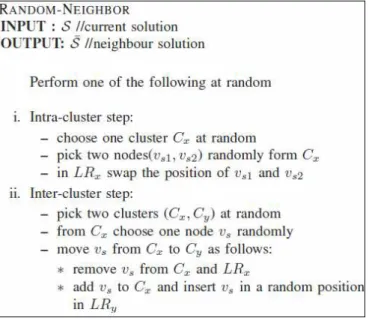
There are three main issues related to the adaptation of the general form approach of III-A to suit the MTSP based problem. i) Generation of the initial random solution for S, at this step, for each node, pick a random cluster and associate to it. ii) The design of the moves and neighborhood structure S̄. S̄ is generated by altering S as shown in Figure. 3. we used two schemes for this purpose. In the first scheme, the algorithm finds a new permutation LR. The second scheme is the partitioning part in the algorithm, where it tries to make the size of the clusters balanced, but also it can help to find the arrangement of nodes in LR, for instance, in case it chooses the same cluster twice this means, it is changing one node position to a new position in the LR. Basically, it is exploring a new permutation of the cluster nodes. iii) The design of the evaluation cost function.

Figure 3. Neighbor generation for MTSP Based algorithm

(5)

is introduced Then the algorithm computes the benefit could be gained or lost by the neighbor solution S̄. The benefit equals ∆ = F (S) − F (S). To reduce the time that is needed to compute ∆. We have proposed to compute only the difference in the gain, instead of recomputed F (S̄) from scratch.

1) Cost function evaluation: Then the cost function F(S) can be computed as follows:

Where fd (LRi) is the cost of distance covered by PRi . fu(ni) is

the entropy term to make the number of nodes inside all the cluster equally distributed. While β is the weighting factor. The algorithm includes user-defined parameter β that can be used to control the size and composition of clusters, either directly or indirectly. The algorithm treats β as an indication of the desirable range of cluster sizes, rather than as hard thresholds that cannot be violated. Consequently, the final result may contain clusters with different sizes.

Computing fd(LR) is the most expensive function in term of

processing power, and it is needed to be performed after exploring a new neighbor solution in the algorithm. So, we have proposed two improvements to cope with this issue, first a simplified version to compute fd(LR), for more

information see subsection IV-A2. Second improvement is to compute fd(LR) only for the changed clusters in the neighbor

solution.

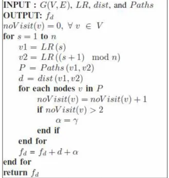
Figure 4. Pseudocode of fd(LR), it computes the cost

function of the physical ring associated with the logical ring

2) Intra-cluster Logical Ring Cost fd(LR): We provide an

algorithm to find the cost (distance length in kilometers) and the components (fiber links, optical nodes) are needed from the physical topology to construct the intra-cluster unidirectional ring PRs. In the i-th cluster, fd (PRi) is the cost

function associated by PRi. For the sake of simplicity we use

LR, PR, and fd, instead of LRi, PRi, and F1 (PRi). The new

algorithm is shown in Figure 4. The idea of the improvement is to avoid computing the shortest path in each iteration. So, the algorithm takes as input Paths that are offline computed.

Resulting in a big reduction in the computation cost needed in each iteration. The noVisit is an array to store the number of time nodes is visited and is set to zeros at initialization. And α is a penalty to be paid if the path between the pair sequence is not a disjoint path. At the end, the algorithm executes n + 1 iterations. Average number of nodes in a single path of Paths is equals |LR|/n, which is 1. Finally, in average it needs O (N+K/K) operations.

4.2. CTNs Selection

Within the scope of this phase inter-cluster mesh identification, we focus on the case that, the network already has been partitioned -regardless of the partitioning approach- into K disjoint cluster. The inter-cluster mesh connects K CTNs by shortest path according to the physical. The problem CTNs Selection is to elect K nodes, such that each node belonging to a different cluster to act as the gateway and the coordinator of the other nodes in the same cluster. In the CANON paradigm context, the interconnection between clusters is made through (CTN). The CTN is a node inside the intra-cluster ring, besides that it is acting as a gateway between it is own cluster and other K − 1 clusters. An equivalent mathematical formulation to CTNs selection problem is the Generalized Subgraph Problem (GSP). The GSP is defined on a graph where the vertex set V is partitioned into K clusters. The task is to find a subgraph which touches at most one vertex in each cluster so as to optimize an objective function. The GSP problem takes only the physical topology as input, and its only goal is to minimize the total inter-CTN distance since it is likely to lead to short light paths between different CTNs, thus requiring fewer wavelengths. Also, this type of solution tends to avoid physical topologies with a large diameter for inter-mesh; such topologies are not a good match for the mesh Topology algorithm which treats each cluster as a virtual mesh. On the other hand, CTN node capacity and traffic routing should also be considered. Specifically, observe that CTNs are responsible for forwarding a larger traffic amount than MEN nodes. Therefore, in order to lower the wavelength requirements for the network as a whole, it is generally desirable to select as CTNs the nodes with the largest bandwidth capacity, i.e., those with the largest physical degree. The GSP problem takes only the physical topology as input, and its only goal is to minimize the total inter-CTN distance and maximize the total CTNs degree. Let us define dist (CTNi, CTNj) the inter-CTN distance from CTNi to CTNj

So, the total inter-CTNs distance is

Similarly, e = E (CTNi) denotes set of links (e) that are

connected to node CTNi that is the node degree. So, the total

CTNs node degree is

(6)

neighborhood structure. The initial random solution by randomly select one node from each cluster and assign it as CTN of that cluster. For the move and neighbor design always in each step select a random cluster and then elect randomly one node to act as CTN for the evaluation function:

maximize (F) F = F 1 − βF 2

Where β is a weighting factor.

5. Routing and Wavelength Assignment

The goal of this phase is in two folds, first to find the routes based on CANON topology, which is the outcome from the previous phase LTD, and secondly to assign the wavelengths in order to carry the traffic between network nodes. Another problem we face in this section is that of grooming the higher-layer traffic. The term grooming is commonly used to refer to the packing of low-speed circuits into higher-speed circuits. In the rest of this section we will discuss several aspects of the design of wavelength-routing networks in some detail. In subsection. V-A, we will compute the Intra-cluster and Inter-cluster physical topologies. In subsection. V-B, we introduce a method for assign wavelength for the Intra-cluster and Inter-cluster connections.

5.1. Routing

According to CANON architecture, the route that carries the traffic between any pair of nodes s Ci and d Cj is

determined based on C i and C j . For instance, the route where t(s, d) passes through the physical topology is defined as follows: if i == j, we have intra-cluster routing that includes all the nodes in the path of ring PRi going from s to

d. If i != j then the route is constructed by three parts: The first segment is the path between s and CTNi in the direction

of the ring LRi . The second is the shortest path between CTNi

and CTNj. And the last segment is the path between CTNj to d

in the direction of LRj.

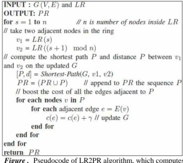
1) Intra-cluster Physical Ring PR: The goal of this algorithm Figure. 5 is to find PR starting from a known LR. The PR is built as a sequence of shortest-paths P. Initially PR = , the algorithm starts from a node of LRv1 and always reaches the

next node of the LRv2, it computes P from v1 to v2 such that

P disjoint with PR. Then it set (PR = PR ∪ P). The algorithm, continue until all the nodes have been touched and the last path closes the cycle. 2) Inter-cluster Physical path: A routes between any pair of CTNs is found based on the shortest path principle using the Dijkstra’s algorithm [9].

5.2. Wavelength Assignment

We emphasize at this stage that we only use the routes which are identified by the previous step regardless of their congestion state. The routing of wavelengths over the physical topology is performed according to CANON paradigm where shortest path principle is not violated. In particular the physical topologies assumed are physical rings utilized for Intra-cluster communications and general mesh that is constructed by shortest paths between any arbitrary CTNs pairs to serve Inter-cluster communications. In this work we consider that the wavelengths in a single fiber are grouped into wavebands. Each fiber link carries F wavebands, each waveband consisting of L consecutive wavelengths. Hence, the total number of wavelengths on each link is W = F × L.

Figure . Pseudocode of LR2PR algorithm, which computes the physical ring

5.3. Intra-cluster Traffic waveband assignment

We now consider a Waveband assignment problem which is defined as follows, Give {PRi}Ki=1 and T(s,d), determine a

route and wavelength(s) for requests, while minimizing the maximum wavelength number is needed by any link in the topology. The wavelength assignment must obey the following constrains: i) two light paths must not be assigned the same wavelength on a given link. ii) If no wavelength conversion is available, then a light path must be assigned the same wavelength on all the links in its route. In physical ring topology set up problem and we examine how it can be solved. We will assume that no connections are imposed by the underlying fiber topology or the optical layer iii) we assume that all light paths are directional similar to the ring direction. iiii) All ring nodes perform grooming wavelength into waveband. All the wavelength grooming do in optical domain without using wavelength conversion. This step considers a single cluster at a time. It has to be carried out K times in order to serve all the intra-cluster communications. At the beginning, we compute T intra traffic matrix. Let us consider the i-th cluster with already elected CTNi,

predefined LRi, and PRi. Thus, T intra is computed as

follows:

Basically, if nodes s and d are not CTN nodes, then T (s, d) is the intra-cluster traffic request amount from node s and node d. If, on the other hand, node d (respectively, node s) is the CTN node, then T iintra(s,d) includes not only the intra

T iintra(s,d) cluster component, but also the aggregate

inter-cluster traffic originating at node s (respectively, terminating at node d). This definition of T iintra(s,d) when either s or d

(7)

In the most general case, T intra (s, d) partially fill all the

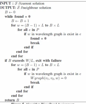
capacity of a whole waveband. So, allow waveband adds and drops at MEN nodes to fill the wavebands pass the nodes in the ring. Which on one hand is minimizing the wavelength cost, but on the other hand is increasing the number of ports. On intra-cluster we proposed an approach which is efficiently combines wavelengths traffic onto a single waveband. The algorithm shown in Figure. 7. Which is based on bin packing problem. The algorithm starts with the method of Figure. 5 to construct the physical ring PR. Then it executes a loop that runs until Tintra is served in its entirety. In each step within the

loop, the algorithm find a free unreserved waveband B using the method which is depicted in Figure. 6. B is covering the whole path of PR on the physical topology. After that, the algorithm tries to fill the whole capacity of B by establishing connections and reducing Tintra by the amount of wavelength

that can be served with the given waveband using the algorithm 8. Light paths into waveband. All light path grooming is per-formed in the optical domain without using wavelength conversion. To further explain the hierarchical model, we use an ex-ample depicted in Figure 2.

Figure 5. Algorithm WaveBand Assignment

Let us assume single wavelength Band paths are established between source and destination nodes using the Rout-The

Tintra matrix is carried over PR, the algorithm in Figure.?? is

used. A free waveband on the PR is identified by the algorithm Figure.??, then the algorithm Figure.8 is used to fill the waveband B with wavelengths and sever all the entry in the matrix. Bandwidths are established over the PR. and the reduction is done.

At the end of intra-cluster, all traffic from the nodes of a cluster Ci with destination outside the cluster, is carried to the

CTNi for transport to the destination CTNj. For K clusters,

with k×k traffic matrix Tinter = [Tinter (Ci, Cj)] where i != j the

inter-cluster traffic matrix defined as

Figure 6. Algorithm Intra-cluster

The algorithm starts with the method of Figure. 5 to construct the physical ring PR. Then it executes a loop that runs until

Tintra is served in its entirety. In each step within the loop, the

algorithm finds a free unreserved waveband B using the method which is depicted in Figure. 6. While in inter-clauter transport we use the second approach where the wavebands mostly filled and just transport them from source CTN to destination CTN without further merging.

Figure 7. Algorithm to fill a WaveBand B with wavelengths

(8)

Figure 8. Pseudocode of Traffic based Clustering

Figure 9. Pseudocode of Traffic based CTN selection

6. Other Algorithms

6.1. K-center based clustering

In this subsection we provide a different approach based on physical distance rather than the traffic matrix to generate the K clusters. This approach is based on well K-Center problem where:

• The input G(V,E) and K;

• The output:

The K-Center problem is NP-Complete [?], [10], and the best approximation ratio that can be obtained in polynomial time is 2 [?], [15]. We use k-center implementation of [10] which is originally aims reduce network cost through hierarchical traffic grooming in WDM networks. In our work, we consider that the CTNs is equivalent hub nodes of [10]. The resulting clusters form k-center have expensive permutation of node

for building logical ring. So, a father stage required to produce cheap permutation of the nodes. We consider this stage to be the ASTP Solver as shown in subsection VI-C.

6.2. Traffic based clustering

Traffic based is an offline heuristic based solution to partition the network nodes into a given number of clusters and eventually define the intra-cluster rings. This heuristic approach based on the traffic matrix rather than physical distance to generate the K clusters and similarly, the K correspondent CTNs.

As an objective, the Traffic-based tries to minimize the intra-cluster traffic exchange. This algorithm considers T, and it does not take into account the physical topology; hence, it may group together nodes that are far apart.

The Traffic-based have two stages:

1 The clustering: Figure. 9 depicts Traffic-based algorithm, it initially start with an empty K clusters and V is a set of N nodes. The algorithm try to grow the K cluster together by adding a node per cluster at time. In each step the T inter is minimized. Break ties by selecting the cluster has the maximum Tintra .

Figure. 10 shows Traffic-based CTNs selection algorithm, for each cluster the algorithm elect the node that is exchanging the largest amount of traffic with nodes belonging to different clusters. And finally to produce the intra-cluster rings {LR i (j)} N

i=1...N, j=1..., n i. The ASTP Solver is used as fully is described in subsection VI-C.

6.3. ATSP Solver

This section presents the ATSP Solver which is used when the clustering phase was done by the K-center or the Traffic based techniques. As an input it takes unordered cluster nodes (e.g. if the clustering was done by the K-center or the Traffic based algorithms) and output the cluster corresponding logical ring LR and physical ring P R. Let j denotes the j-th node in a network, and AT SP (Ci) denotes

ATSP Solver with the input being the Ci. The benefit

function B and the cost function F1 for solving the ATSP (Ci)

are defined by the following equations:

Where, μj is a benefit of including j in the solution, γ is a large enough real value to ensure that all nodes in Ci will be

included in the final PRi, β is a weighting factor. Nj is

function equals when the j-node is included in PRi . F 1 (PRi )

(9)

modification is needed to be introduced to ESA so it suits our problem. That is to optimize our cost function F.

7. Numerical results

In this section, we present experimental results to demonstrate the function and performance of our clustering algorithms.

7.1. Reference network topologies

The experiments were applied on two different network topologies: Figures 11 and 12 represent the used network topologies, in the two figures nodes shown as circles and the lines between circles represent the links of the network topology; more over the number inside each circle is the ID of the correspondent network node. For all the three networks the total area considered in are scaled to fit into a unit area. To compute the distance between directly connected cities in the network the latitude and longitude and we used plane approximation method described in [11]. And this distance stored in D but in case there is no link between the cities the distance is equal to shortest path distance. The first topology is the Pan-European core; The Pan-European core network consists of 16 nodes and 23 links.

Figure 10. Large Pan-European network topology

Figure 11. IDEAL Network topology

The nodes were chosen in such a way that they include some of the European Internet Exchange Points; and the second topology is an extended version from the first one where more European countries is added to the first network and we call it Large Pan-European network topology, which is shown in Figure. 11; The large topology consist of 37 nodes and 47 links.

The third topology is an ideal topology network and it is schematically shown in Figure 12. This topology consists 64 nodes and 120 links; It is pointed out that the Ideal topology provides for more connectivity i.e. it has a higher number of links.

7.2. Traffic load profiles

We consider both fixed and random traffic scenarios. Let ρ

be the input load at each source node, and tij the load from

source node i to destination node j (T = [tij] is called the

traffic matrix). The traffic matrix of each problem instance we consider is generated by drawing N × (N −1) float numbers. Nodes inside the network do not exchange traffic between them self so in all scenarios [tij] = 0.0 if i = j. To

illustrate that our approach works well for different traffic patterns, we consider four patterns in our study:

• Fixed traffic pattern. we assign a fix float number of all the elements of the traffic matrix, [tij] = ρ. Fixed

traffic matrix does not have any particular structure that takes into account the geographical a proximity between nodes, and nodes exchange deterministic amount of traffic with all other nodes in their cluster or out of their cluster, so in this case there are no benefits from taking in account traffic matrix in the proposed clustering algorithms.

• Uniform random pattern. This pattern is a standard practice among researchers used to assess any network algorithm under such scenario. To generate a uniform random traffic matrix for a problem instance, we drawn N × (N − 1) float numbers from uniform distribution, where the values fall in the traffic elements take values in a wide range in the interval, and loads of individual links also vary widely.

We have found that random patterns are often challenging in the context of network hierarchical clustering algorithm since the matrix does not have any particular structure that can be exploited by the algorithm. Nearest traffic pattern. This pattern is such that nodes physically close to each other exchange more traffic than nodes far away from each other. Specifically, the node pair with minimum physical distance between all possible nodes pair in the network will exchange among them self the largest amount of traffic, let dmin be the

minimum possible distance between all nodes pair in the network and dij is the shortest path distance

(10)

• Farthest traffic pattern. This is the opposite of the nearest pattern in pattern nodes physically far away from each other exchange more traffic than nodes close to each other. In fact, the node pair with the maximum shortest path physical distance between all possible nodes pair in the network will exchange among them self the largest amount of traffic, let dmax to be the maximum possible shortest path

distance between all nodes pair in the network and dij is the shortest path distance between node i and

node j, then the overspending node pair will exchange h load from uniform distribution, where values fall in

7.3. Network Cost

We assume that there are two types of optical cross-connect (OXC) in the network. The first group which is used in CTNs. The second is used in Metro-Edge Nodes (MENs). All the nodes belonging to the same group have exactly the same capabilities (i.e., in terms of switching and grooming capability). Clearly, the number of clusters, their composition, and the corresponding CTNs must be selected in a way that helps achieve our goal of minimizing the total number of optical ports and wavelengths required to carry the traffic demands. Therefore, the way of building the clusters and CTNs is a complex and difficult task, as it depends on both the physical topology of the network and the traffic matrix. To illustrate this point, consider the tradeoffs involved in determining the number of clusters. If is very small, the amount of inter-cluster traffic generated by each cluster will likely be large. Hence, the CTNs may become bottlenecks, resulting in a large number of optical ports at each CTN and possibly a large number of wavelengths since many light paths may have to be carried over the fixed number of links to/from each CTN. On the other hand, a large value for implies a small number of nodes within each cluster. In this case, the amount of intra-cluster traffic will be small, resulting in inefficient filled Waveband. Similarly, at the second-level cluster, paths will have to be set up to carry small amounts of inter-cluster traffic.

In this work we consider that the wavelengths in a single fiber are grouped into wavebands. Each fiber link carries F wavebands, each waveband consisting of L consecutive wavelengths. Hence, the total number of wavelengths (W) on each link is W = F × L. The first approach encourages waveband merges and splits, a number of bands are dropped to the WXC layer before being added back to the BXC layer again. This increases the number of ports needed at the nodes where waveband merges/splits take place. The second the hierarchical approach, band merges and splits are not allowed. The bands are routed between source and destination without modification. As a result, the first approach uses more ports than the second approach. On the other hand, the first using less number of wavelengths. In the considered hierarchical model, CTNs mostly originating and terminating a larger number of wavelengths than MEN nodes. So, the traffic between CTN s should be transported in bulk quantities like wavebands. While connection requests in wavelength routed inside a single cluster often require less capacity than is available on a single Waveband. Based on

the previous observation: we propose for this hierarchical approach can be for intra-cluster transport we use the first approach which aims to combine wavelength into waveband in all the ring nodes. While in inter-claster transport we use the second approach where the wavebands mostly filled and just transport them from source CTN to destination CTN without further merging. During this phase, we first divide the traffic matrix T into two different types: The first class represent the intra-cluster communication. And the second is inter-cluster communication.

Figure 12. Illustrates the relation between number of hops

and number of Clusters using Simulated Annealing and K-center algorithms

Figure 13. Illustrates the relation between distance and

number of Clusters using Simulated Annealing and K-center algorithms

Figure 14. Illustrates the average number of hops while

changing number of Clusters using Simulated Annealing and K-center algorithms

(11)

8. Conclusions

Network design process is very important in order to balance between the investment in the network and the supervises offered to the network user, taking into consideration, both minimizing the network investment cost, on the other hand, maximizing the quality of service offered to the customers as well. Partitioning the network to smaller sub-networks called clusters is required during the design process in order to ease studying the whole network and achieve the design process as a trade-off between several attributes such as quality of service, reliability, cost, and management. Under CANON, a large scale optical network is partitioned into a number of geographically limited areas taking into account many different criteria like administrative domains, topological characteristics, traffic patterns, legacy infrastructure, … etc. An important consideration is that each of these clusters is comprised of a group of nodes in geographical proximity. The clusters can coincide with administrative domains but there could be many cases where two or more clusters belong to the same administrative domain. Therefore, in the most general case the partitioning into specific clusters can be either an off-line or an on-line process.

In this work only the off-line case is considered. In this Study, we look at the problem of designing efficient 2-level Hierarchical Optical Networks (HON), in the context of network costs optimization. 2-level HON paradigm only have local rings to connect disjoint sets of nodes and a global sub mesh to interconnect all the local rings. We present a Hierarchical algorithm that is based on two phases. We present results for scenarios containing a set of real optical topologies.

References

[1] Che, Xianhui, "Overview of optical local access networks development and design challenges." International Journal of Communication Networks and Information Security, Vol 2, no. 1, pp.35, 2010.

[2] Róka, Rastislav, and Martin Mokrán. "Modeling of the PSK utilization at the signal transmission in the optical transmission medium." International Journal of Communication Networks and Information Security, Vol 7, no. 3, pp .187, 2015.

[3] K. Srinivasarao and R. Dutta, “Traffic-partitioning approaches to grooming ring networks,” in Autonomic and Autonomous Systems and International Conference on Networking and Services, 2005. ICAS-ICNS 2005. Joint International Conference on, p. 6, oct. 2005.

[4] S. Yadlapalli, W. Malik, S. Darbha, and M. Pachter, “A lagrangian-based algorithm for a multiple depot, multiple travelling salesmen problem,” in American Control Conference, 2007. ACC ’07, pp. 4027–4032, July 2007. [5] S. Kirkpatrick, C. D. Gelatt, and M. P. Vecchi, “Optimization

by simulated annealing,” Science, vol. 220, no. 4598, pp. 671–680, 1983. [Online]. Available:

http://www.sciencemag.org/content/220/4598/671.abstract , last-accessed August, 2016.

[6] V. ern, “Thermodynamical approach to the traveling salesman problem: An efficient simulation algorithm,” Journal of Optimization Theory and Applications, vol. 45, pp. 41–51, 1985.

[7] C.-H. Song, K. Lee, and W. D. Lee, “Extended simulated annealing for augmented tsp and multi-salesmen tsp,” in Neural Networks, 2003.

[8] Proceedings of the International Joint Conference on, vol. 3, pp. 2340 – 2343, July 2003.

[9] T.-H. Kim, C.-H. Song, W. D. Lee, and J.-C. Ryou, “Building a packages delivery schedule using extended simulated annealing,” in Neural Networks, 2006. IJCNN ’06. International Joint Conference on, 0-0, pp. 2691 –2695, 2006. [10] T. Bektas, “The multiple traveling salesman problem: an

overview of formulations and solution procedures,” Omega, vol. 34, no. 3, pp. 209–219, June 2006. [Online]. Available: http://ideas.repec.org/a/eee/jomega/v34y2006i3p209-219.html , last-accessed August, 2016.

[11] C. Feremans, M. Labbe, A. Letchford, and J. J. Salazar, “The generalized subgraph problem: Complexity, approximability and polyhedra,” 2003.

[12] E. W. Dijkstra, “A note on two problems in connexion with graphs,” Nu-merische Mathematik, vol. 1, pp. 269–271, 10.1007/BF01386390, 1959.

[13] B. Chen, G. Rouskas, and R. Dutta, “On hierarchical traffic grooming in wdm networks,” Networking, IEEE/ACM Transactions on, vol. 16, no. 5, pp. 1226 –1238, oct. 2008. [14] L. Sun, “pos2dist,”