Generalized global symmetries and dissipative magnetohydrodynamics
Sašo Grozdanov,1,* Diego M. Hofman,2,† and Nabil Iqbal2,‡ 1Instituut-Lorentz for Theoretical Physics, Leiden University,
Niels Bohrweg 2, Leiden 2333 CA, Netherlands
2Institute for Theoretical Physics, University of Amsterdam, Science Park 904,
Postbus 94485, 1090 GL Amsterdam, Netherlands (Received 2 January 2017; published 5 May 2017)
The conserved magnetic flux of Uð1Þ electrodynamics coupled to matter in four dimensions is associated with a generalized global symmetry. We study the realization of such a symmetry at finite temperature and develop the hydrodynamic theory describing fluctuations of a conserved 2-form current around thermal equilibrium. This can be thought of as a systematic derivation of relativistic magneto-hydrodynamics, constrained only by symmetries and effective field theory. We construct the entropy current and show that at first order in derivatives, there are seven dissipative transport coefficients. We present a universal definition of resistivity in a theory of dynamical electromagnetism and derive a direct Kubo formula for the resistivity in terms of correlation functions of the electric field operator. We also study fluctuations and collective modes, deriving novel expressions for the dissipative widths of magnetosonic and Alfvén modes. Finally, we demonstrate that a nontrivial truncation of the theory can be performed at low temperatures compared to the magnetic field: this theory has an emergent Lorentz invariance along magnetic field lines, and hydrodynamic fluctuations are now parametrized by a fluid tensor rather than a fluid velocity. Throughout, no assumption is made of weak electromagnetic coupling. Thus, our theory may have phenomenological relevance for dense electromagnetic plasmas.
DOI:10.1103/PhysRevD.95.096003
I. INTRODUCTION
Hydrodynamics is the effective theory describing the long-distance fluctuations of conserved charges around a state of thermal equilibrium. Despite its universal utility in everyday physics and its pedigreed history, its theoretical development continues to be an active area of research even today. In particular, the new laboratory provided by gauge/ gravity duality has stimulated developments in hydrody-namics alone, including an understanding of universal effects in anomalous hydrodynamics [1–3], potentially fundamental bounds on dissipation[4,5], a refined under-standing of higher-order transport[6–12], and path-integral (action principle) formulations of dissipative hydrodynam-ics[13–21]; see e.g. Refs.[5,22,23] for reviews of hydro-dynamics from the point of view afforded by holography. It is well understood that the structure of a hydrodynamic theory is completely determined by the conserved currents and the realization of such symmetries in the thermal equilibrium state of the system. In this paper, we would like to apply such a symmetry-based approach to the study of magnetohydrodynamics, i.e. the long-distance limit of Maxwell electromagnetism coupled to light charged matter at finite temperature and magnetic field.
To that end, we first ask a question with a seemingly obvious answer: what are the symmetries ofUð1Þ electro-dynamics coupled to charged matter? One might be tempted to say that there is a Uð1Þ currentjμel associated with electric charge. There is indeed such a divergenceless object, related to the electric field strength by Maxwell’s equations:
1 g2∇μF
μν¼jν
el: ð1:1Þ
However, the symmetry associated with this current is a gaugesymmetry. Gauge symmetries are merely redundan-cies of the description and thus are presumably not useful for organizing universal physics.
The true global symmetry of Uð1Þ electrodynamics is actually something different. Consider the following anti-symmetric tensor:
Jμν¼1
2εμνρσFρσ: ð1:2Þ
It is immediately clear from the Bianchi identity (i.e. the absence of magnetic monopoles) that ∇μJμν¼0. This is not related to the conservation of electric charge but rather states that magnetic field lines cannot end.
What is the symmetry principle behind such a conser-vation law? It has recently been stressed in Ref.[24]that just as a normal 1-form current Jμ is associated with a *[email protected]
global symmetry, higher-form symmetries such as Jμν are associated withgeneralized global symmetriesand should be treated on precisely the same footing. We first review the physics of a conventional global symmetry, which we call a 0-form symmetry in the notation of Ref. [24]: with every 0-form symmetry comes a divergenceless 1-form current jμ, the Hodge dual of which we integrate over a codi-mension-1 manifold to obtain a conserved charge. If this codimension-1 manifold is taken to be a time slice, then the conserved charge can be conveniently thought of as counting a conserved particle number: intuitively, since particle world lines cannot end in time, we can“catch”all the particles by integrating over a time slice. The objects that are charged under 0-form symmetries are local oper-ators which create and destroy particles, and the symmetry acts [in theUð1Þcase] by multiplication of the operator by a 0-form phase Λ that is weighted by the charge of the operatorq: OðxÞ→eiqΛOðxÞ.
Consider now the less familiar but directly analogous case of a 1-form symmetry. a 1-form symmetry comes with a divergenceless 2-form currentJμν, the Hodge star of which we integrate over a codimension-2 surface to obtain a conserved chargeQ¼RS⋆J. This conserved charge should be thought of as counting astringnumber: as strings do not end in spaceorin time, an integral over a codimension-2 surface is enough to catch all the strings,1as shown in Fig.1. The objects that are charged under 1-form symmetries are one-dimensional (1D) objects such as Wilson or’t Hooft lines. These 1D objects create and destroy strings, and the symmetry acts (in the 1-form case) by multiplication by a 1-form phase Λμ integrated along the contour Cof the’t Hooft line:WðCÞ→expðiqRCΛμdxμÞWðCÞ.
In the case of electromagnetism, the 2-form current is given by(1.2), and the strings that are being counted are magnetic field lines. We could also consider the dual current Fμν itself, which would count electric flux lines; however, from(1.1), we see thatFμνis not conserved in the presence of light electrically charged matter, because electric field lines can now end on charges. Thus, electro-dynamics coupled to charged matter has only a single conserved 2-form current. This is the universal feature that distinguishes theories of electromagnetism from other theories, and the manner in which the symmetry is realized should be the starting point for further discussion of the phases of electrodynamics.2For example, this symmetry is spontaneously broken in the usual Coulomb phase (where the gapless photon is the associated Goldstone boson) and
is unbroken in the superconducting phase (where magnetic flux tubes are gapped). We refer the reader to Ref.[24]for a detailed discussion of these issues.
In this paper, we discuss the long-distance physics of this conserved currentnear thermal equilibrium, applying the conventional machinery of hydrodynamics to a theory with a conserved 2-form current and conserved energy momentum. We are thus constructing a generalization of the (very well-studied) theory that is usually called rela-tivistic magnetohydrodynamics. To the best of our knowl-edge, most discussions of magnetohydrodynamics (MHD) separate the matter sector from the electrodynamic sector. It seems to us that this separation makes sense only at weak coupling and may often not be justified; for example, the plasma coupling constantΓ, defined as the ratio of potential to kinetic energies for a typical particle, is known to attain values up toOð102Þin various astrophysical and laboratory plasmas[26]. Experimental estimates of the ratio of shear viscosity to entropy density (where a small value is widely understood as being a universal measure of interaction strength [4]) in such plasmas at high Γ obtain minimum values that are Oð1Þ−Oð10Þ [27]. These suggest the presence of strong electromagnetic correlations.
Our discussion will not make any assumptions of weak coupling and should therefore be valid for any value ofΓ; we will be guided purely by symmetries and the principles of the effective field theory of hydrodynamics. Beyond the (global) symmetries, the construction of the hydrodynamic gradient expansions also requires us to choose relevant hydrodynamic fields (degrees of freedom), which, as we will discuss, crucially depend on the symmetry breaking pattern in the physical system at hand. In particular, in addition to conventional hydrodynamics at finite temperature, we will also study a variant of magnetohydrodynamics at very low temperatures. This theory has an emergent Lorentz invari-ance associated with boosts along the background magnetic field lines, and the parametrization of hydrodynamic fluc-tuations is considerably different. Interestingly, atT ¼0, leading-order corrections to ideal hydrodynamics only enter at second order, thus showing the direct relevance of higher-order hydrodynamics (see e.g. Refs.[6,8,9,11]). While this treatment does not include the typical light modes that FIG. 1. Integration over a codimension-2 surfaceScounts the number of strings that cross it at a given time.
1
Note that the dynamics of stringlike degrees of freedom has been discussed in the context of superfluid hydrodynamics in the interesting recent paper[25]. In that case, strings arise as solitons and, unlike in our work, interact through long range forces.
2
emerge atT ¼0, it does capture a universal self-contained sector of magnetohydrodynamics.
We now describe an outline of the rest of this paper. In Sec.II, we discuss the construction of ideal hydrodynamic theory at finite temperature. In Sec.III, we move beyond ideal hydrodynamics: we work to first order in derivatives and demonstrate that there are seven transport coefficients that are consistent with entropy production, describing also how they may be computed through Kubo formulas. In Sec.IV, we study linear fluctuations around the equilibrium solution and derive the dispersion relations and dissipative widths of gapless magnetohydrodynamic collective modes. In Sec. V, we study the simple extension of the theory associated with adding an extra conserved 1-form current (e.g. baryon number). In Sec.VI, we turn to the theory at strictly zero temperature, where we discuss novel phenom-ena that can be understood as arising from a hydrodynamic equilibrium state with extra unbroken symmetries. We conclude with a brief discussion and possible future applications in Sec.VII.
Previous study of the hydrodynamics of a fluid of strings includes Ref.[28]. While this work was being written, we came to learn of the interesting paper [29], which also studies a dissipative theory of strings and makes the connection to MHD. Though the details of some deriva-tions differ, there is overlap between that work and our Secs. II andIII.
II. IDEAL MAGNETOHYDRODYNAMICS
Our hydrodynamic theory will describe the dynamics of the slowly evolving conserved charges, which in our case are the stress-energy tensor Tμν and the antisymmetric currentJμν.
A. Coupling external sources
For what follows, it will be very useful to couple the system to external sources. The external source for the stress-energy tensor is a background metricgμν, and we also couple the antisymmetric currentJμνto an external 2-form gauge field source bμν by deforming the microscopic on-shell actionS0 by a source term:
S½b≡S0þΔS½b;
ΔS½b≡
Z
d4xpffiffiffiffiffiffi−gbμνJμν: ð2:1Þ
The currents are defined in terms of the total action as
TμνðxÞ≡ 2ffiffiffiffiffiffi
−g p δS
δgμνðxÞ; ð2:2Þ
JμνðxÞ≡ 1ffiffiffiffiffiffi
−g p δS
δbμνðxÞ: ð2:3Þ
Demanding invariance of this action under the gauge symmetry δΛb¼dΛ with Λ a 1-form gauge parameter results in
∇μJμν¼0: ð2:4Þ
Similarly, demanding invariance under an infinitesimal diffeomorphism that acts on the sources as a Lie derivative,
δξg¼Lξg,δξb¼Lξb, gives us the (non)conservation of the stress-energy tensor in the presence of a source,
∇μTμν¼HνρσJρσ; ð2:5Þ
where H¼db. The term on the right-hand side of the equation states that an external source can perform work on the system.
We now discuss the physical significance of theb-field source. A termbti¼μshould be thought of as a chemical
potential for the chargeJti, i.e. a string oriented in theith
spatial direction.
For our purposes, we can obtain some intuition by considering the theory of electrodynamics coupled to such an external source, i.e. consider using (1.2) to write the current as
Jμν¼εμνρσ∂ρAσ; ð2:6Þ
withAthe familiar gauge potential from electrodynamics.3 Then, the coupling(2.1) becomes after an integration by parts
ΔS½b ¼ Z
d4xpffiffiffiffiffiffi−gAσjσext;
jσext≡εσρμν∂ρbμν: ð2:7Þ
The field strengthHassociated tobcan be interpreted as an externalbackground electric charge density to which the system responds.
For example, consider a cylindrical region of space V that has a nonzero value for the chemical potential in thez direction,
btzðxÞ ¼ μ
2θVðxÞ; ð2:8Þ
whereθVðxÞis 1 ifx∈V and is 0 otherwise. Then, from (2.7), we see that we have
jϕextðxÞ ¼μδ∂VðxÞ; ð2:9Þ
i.e. we have an effective electric current running in a delta-function sheet in theϕ direction along the outside of the cylinder. Thus, the chemical potential for producing a
3We choose conventions wherebyε
magnetic field line poking through a system is an electrical current running around the edge of the system, as one would expect from textbook electrodynamics. In our formalism, the actual magnetic field created by this chemical potential is controlled by a thermodynamic function, the susceptibility for the conserved charge density Jtz.
We will sometimes return to the interpretation of b as charge source to build intuition; however, we stress that in general when there are light electrically charged degrees of freedom present, the AðxÞ defined in (2.6) does not have a local effective action and is not a useful quantity to consider.
B. Hydrodynamic stress-energy tensor and current
We now turn to ideal hydrodynamics at nonzero temper-ature. We first discuss the equilibrium state. Recall that the analog of a conserved chargeQfor our 2-form current is its integral over a codimension-2 spacelike surfaceSwith no boundaries, as shown in Fig.1,
Q¼ Z
S
⋆J: ð2:10Þ
Qcounts the number of field lines crossingSat any instant of time and is thus unaltered by deformations ofSin both space and time. A thermal equilibrium density matrix is then given (for a particular choice ofS) by
ρðT;μÞ ¼exp
−1
TðH−μQÞ
; ð2:11Þ
where μ is the chemical potential associated with the 2-form charge. This density matrix can be obtained from cutting open a Euclidean path integral with an appropriate component ofbturned on, e.g. theSis thexyplane then we would use btz ¼μ2.
Elementary arguments, which we spell out in detail in Appendix A, then give us the form of the stress-energy tensor and the conserved higher rank current in thermal equilibrium4:
Tμνð0Þ¼ ðεþpÞuμuνþpgμν−μρhμhν;
Jμνð0Þ¼2ρu½μhν; ð2:12Þ
satisfying the conservation equations in the ideal limit
∇μTμνð0Þ ¼0; ∇μJμνð0Þ ¼0: ð2:13Þ
We have labeled this expression with a subscript 0, as this will be only the zeroth-order term in an expansion in derivatives. Here,uμis the fluid velocity as in conventional hydrodynamics.hμis the direction along the field lines, and we impose the following constraints:
uμuμ¼−1; hμhμ¼1; hμuμ¼0: ð2:14Þ
It will also often be useful to use the projector onto the two-dimensional subspace orthogonal to bothuandh,
Δμν¼gμνþuμuν−hμhν; ð2:15Þ
with traceΔμμ¼2. In(2.12)and whereρis the conserved flux density andpis the pressure. There is no mixeduμhν term, as this can be removed with no loss of generality by a Lorentz boost in theðu; hÞplane.5
Note the presence of thehμhν term in the stress-energy tensor, representing the tension in the field lines. Its coefficient in equilibrium is μρ. It is a bit curious from the effective field theory perspective that this coefficient is fixed and is not given by an equation of state, likep, for example. There is a quick thermodynamic argument to explain this fact. Consider the variation of the internal energy for a system containing field lines running perpen-dicularly to a cross section of areaA, with an associated tension τ and a conserved charge Q given by the flux through the section,
dU¼TdS−pdVþτAdLþμLdQ; ð2:16Þ
where L is the length of the system perpendicular to A. BecauseQis a charge defined by an area integral, it is given byQ¼ρA, and the factor ofLin front ofdQis the correct scaling with the height of the system. Now, perform a Legendre transform to the Landau grand potential,
Φ¼U−TS−μLQ; ð2:17Þ
dΦ¼−sVdT−pdV−ρVdμþ ðτ−μρÞAdL; ð2:18Þ
wheresis the entropy density. Notice thatΦis the quantity naturally calculated by the on-shell action, and we expect it to scale with volume in local quantum field theory. This scaling is spoiled by the term proportional to dL unless τ¼μρ. This condition is, therefore, enforced by extensivity.
4Equilibrium thermodynamics in the presence of magnetic fields has also recently been studied in Ref.[30]; that work differs from ours in that the magnetic fields there are fixed external sources for a conventional 1-form current, whereas in our case the magnetic fields are themselves the fluctuating degrees of freedom of a 2-form current.
The thermodynamics is, thus, completely specified by a single equation of state, i.e. by the pressure as a function of temperature and chemical potential pðT;μÞ. The relevant thermodynamic relations are
εþp¼Tsþμρ; dp¼sdTþρdμ; ð2:19Þ
withsthe entropy density. Here, we have made use of the volume scaling assumption.
The microscopic symmetry properties of J do not actually determine those of hμ and ρ, only that of their product. In this work, we assume the charge assignments in TableI, which are consistent with magnetohydrodynamical intuition and are particularly convenient. Note that all scalar quantities (such asρandμ) are taken to have even parity under all discrete symmetries, and charge conjugation is taken to flip the sign of h. These symmetries will play a useful role later on in restricting corrections to the entropy current.
Hydrodynamics is a theory that describes systems that are in local thermal equilibrium but can globally be far from equilibrium, in which case the thermodynamic degrees of freedom become space-time-dependent hydrodynamic fields. Thus, the degrees of freedom are the two vectors uμ,hμand two thermodynamic scalars which can be taken to be μ and T, leading to 7 degrees of freedom. The equations of motion are the conservation equations (2.5)
and(2.4). As Jis antisymmetric, one of the equations for the conservation ofJdoes not include a time derivative and is a constraint on initial data. This constraint is consistently propagated by the remaining equations of motion, thus leaving effectively six equations for six variables, and the system is closed.
We now demonstrate that the equations of motion of ideal hydrodynamics result in a conserved entropy current. Consider dotting the velocity u into the conservation equation for the stress-energy tensor (2.5). Using the thermodynamic identities (2.19), we find
uν∇μTμν¼−T∇μðsuμÞ−μ∂μðρuμÞ
−μρðuν∇μhνÞhμ¼0: ð2:20Þ
We now project the conservation equation forJ alonghμ:
hν∇μJμν¼∇μðρuμÞ−ρhμð∇μuνhνÞ ¼0: ð2:21Þ
Inserting this into (2.20) and using ∇μðuνhνÞ ¼0 to rearrange derivatives, we find
∇μðsuμÞ ¼0: ð2:22Þ
We thus see that the local entropy currentsuμis conserved, as we expect in ideal hydrodynamics.
We now turn to the interpretation of the other compo-nents of the hydrodynamic equations. The projections of
(2.5)alonghν andΔνσ, respectively, are
hν½ðεþpÞuμ∇μuνþ∇νp−∇μðμρhμÞ ¼0; ð2:23Þ
Δνσ½ðεþpÞuμ∇μuνþ∇νp−μρhμ∇μhν ¼0: ð2:24Þ
These are the components of the Euler equation for fluid motion in the direction parallel and perpendicular to the background field.
Similarly, the evolution of the magnetic field is given by the projection of the conservation equation forJμνalonghν in(2.21)and along Δνσ below:
Δνσðuμ∇μhν−hμ∇μuνÞ ¼0: ð2:25Þ
The equation states that the transverse part of the magnetic field is Lie dragged by the fluid velocity.
This is the most general system that has the symmetries of Maxwell electrodynamics coupled to charged matter. In particular, unlike conventional treatments of MHD, we have made no assumption that theUð1Þgauge couplingg2 is weak. Indeed, it appears nowhere in our equations; in theories with light charged matter, the fact that g2 runs means that it does not have a universal significance and will not appear as a fundamental object in hydrodynamic equations.
To make contact with the traditional treatments of MHD, consider expanding the pressure in powers ofμ, e.g.
pðμ; TÞ ¼p0ðTÞ þ1
2gðTÞ2μ2þ : ð2:26Þ
Here, p0ðTÞ should be thought of as the pressure of the matter sector alone. The expansion is given in powers ofμ2, as the sign ofμis not physical.6If we stop at this order and then further assume that the coefficient of theμ2 term is independent of temperature gðTÞ ¼g, then the theory of ideal hydrodynamics arising from this particular equation of state is entirely equivalent to traditional relativistic MHD with gauge coupling given byg. From our point of view, this is then a weak-magnetic-field limit of our more general theory. Note that this weak-field limit is entirely different from the hydrodynamic limit that we are taking throughout TABLE I. Charges under discrete symmetries of 2-form current
and hydrodynamical degrees of freedom.
Jti Jij ut ui ht hi ρ,μ,ε,p
C − − þ þ − − þ
P þ − þ − − þ þ
T − þ þ − þ − þ 6In this theory, the sign of the magnetic field is carried by the
this paper, and there is an entirely consistent effective theory even if we do not take the weak-field limit. We discuss some physical consequences of keeping higher-order terms in this expansion (which will be generically present in any interacting theory, even if their coefficient may be small under particular circumstances) later on in this paper.
Nevertheless, if we truncate the expansion for the pressure as in (2.26), then we find from (2.19): ρ¼g2μ and ε¼ε0þ2ρg22 with ε0¼T∂Tp0ðTÞ−p0. The ideal
hydrodynamic theory of our 2-form current is now entirely equivalent to conventional treatments of ideal MHD, as presented in e.g. Ref. [33]. As s∼∂Tp, the T
-independ-ence ofgand thus of theμ-dependent piece of the pressure essentially means that the magnetic field degrees of free-dom carry no entropy.
III. FIRST-ORDER HYDRODYNAMICS
Hydrodynamics is an effective theory, and thus(2.12)are only the zeroth-order terms in a derivative expansion. We now move on to first order in derivatives; to be more precise, the full stress-energy tensor is given by
Tμν¼Tμνð0ÞþTμνð1Þþ ; ð3:1Þ
Jμν¼Jμνð0ÞþJμνð1Þþ ; ð3:2Þ
where the zeroth-order term is given by the ideal MHD expressions in(2.12), and our task now is to determine the first-order corrections as a function of the fluid variables such as the velocity and magnetic field. The numbers that parametrize these corrections are the transport coefficients such as viscosity and resistivity. The physics of dissipation and entropy increase enter at first order in the derivative expansion; as usual in hydrodynamics, the possible tensor structures that can appear (and thus the number of inde-pendent transport coefficients) are greatly constrained by the requirement that entropy always increases.
A. Transport coefficients
We follow the standard procedure to determine these corrections [34]. We begin by writing down the most general form for the first-order terms:
Tμνð1Þ ¼δεuμuνþδfΔμνþδτhμhνþ2lðμhνÞ
þ2kðμuνÞþtμν;
Jμνð1Þ ¼2δρu½μhνþ2m½μhνþ2n½μuνþsμν: ð3:3Þ
Here,lμ; kμ; mμ, andnμare transverse vectors (i.e. orthogo-nal to both uμ and hμ); tμν is a transverse, traceless, and symmetric tensor; and sμν is a transverse, antisymmetric tensor.
Next, we exploit the possibility of changing the hydro-dynamical frame. In hydrodynamics, there is no intrinsic microscopic definition of the fluid variablesfuμ; hμ;μ; Tg. Each field can therefore be infinitesimally redefined, as e.g. uμðxÞ→uμðxÞ þδuμðxÞ. The microscopic currents and the stress-energy tensor must remain invariant under this operation, and thus the redefinition alters the functional form of the relationship between the currents and the fluid variables. In conventional hydrodynamics of a charged fluid, this freedom is often used to setTμνð1Þuν¼0(Landau frame) orjμð1Þ¼0 (Eckart frame). We will use the scalar redefinitions ofμandTto setδρ¼δε¼0and the vector redefinitions ofuμandhμto setkμ¼nμ¼0. We now have the simpler expansion:
Tμνð1Þ¼δfΔμνþδτhμhνþ2lðμhνÞþtμν; ð3:4Þ
Jμνð1Þ¼2m½μhνþsμν: ð3:5Þ
Our task now is to determine the form of the reduced set fδf;δτ;lμ; mμ; tμν; sμνgin terms of derivatives of the fluid variables.
To proceed, we require an expression for the nonequili-brium entropy current Sμ. The textbook approach to this problem is to postulate a standard“canonical”form for this entropy current, motivated by promoting the thermody-namic relationTs¼pþε−μρto the following covariant expression:
TSμ¼puμ−Tμνuν−μJμνhν: ð3:6Þ
Up to first order in derivatives, this is equivalent to
Sμ¼suμ−1 TT
μν
ð1Þuν−μTJðμν1Þhν: ð3:7Þ
We will take this to be our entropy current. As in conven-tional hydrodynamics[35], one can show that it is invariant under frame redefinitions of the sort described above.
Next, we directly evaluate the divergence ∇μSμ. Using the contraction of the conservation Eqs.(2.5)and(2.4)with uμ, we find after some straightforward algebra
∇μSμ¼−
Tμνð1Þ∇μ
uν
T
þJμνð1Þ
∇μ
hνμ
T
þuσHσμν T
:
ð3:8Þ
requiring that the dissipative corrections take the following form,
lμ¼−2η
∥Δμσhν∇ðσuνÞ; ð3:9Þ
tμν¼−2η⊥
ΔμρΔνσ−1
2ΔμνΔρσ
∇ðρuσÞ; ð3:10Þ
mμ¼−2r⊥Δμβhν
T∇½β
hνμ T
þuσHσβν
; ð3:11Þ
sμν¼−2r∥ΔμρΔνσðμ∇½ρhσþHλρσuλÞ; ð3:12Þ
where the four transport coefficientsη⊥;∥andr⊥;∥must all be positive.
In the bulk channel parametrized byδfandδτ, mixing is possible. The most general allowed form that is consistent with positivity is parametrized by three transport coeffi-cients ζ⊥;∥;×:
δf¼−ζ⊥Δμν∇μuν−ζ×hμhν∇μuν ð3:13Þ
δτ¼−ζ×Δμν∇μuν−ζ∥hμhν∇μuν: ð3:14Þ
Note that this mixing matrix is symmetric, in that the mixing termζ×is the same forδfandδτ. This follows from an Onsager relation on mixed correlation functions, as we explain in Sec. III Bbelow.7
Further demanding that the right-hand side of(3.8)be a positive-definite quadratic form imposes two constraints on the bulk viscosities, which may be written as
ζ⊥ ≥0 ζ⊥ζ∥≥ζ2×: ð3:15Þ
There are no further constraints that we know of. At first order, we thus have seven transport coefficientsζ⊥;∥;×,η⊥;∥ andr⊥;∥. If we were to allow all coefficients permitted by symmetries, we would instead have concluded that there were 11 independent transport coefficients consistent with the parity assignments under hμ→−hμ, illustrating the constraints enforced by the second law of thermodynamics. We now turn to the interpretation of these transport coefficients. It is clear that ζ⊥;∥;× andη⊥;∥are anisotropic bulk and shear viscosities, respectively; for a charged fluid in a fixed external magnetic field, one finds instead seven independent viscosities [37], where the difference in counting arises from the fact that we have imposed a charge-conjugation symmetryhμ→−hμ.
The transport coefficients r∥;⊥ can be interpreted as the conventional electrical resistivity parallel and perpendicular to the magnetic field. To understand this, first note that the familiar electric field Eμ is defined in terms of the electromagnetic field strength asEμ¼Fμνuν. Using(1.2), we find
Eμ¼−1
2εμνρσuνJρσ ¼−1
2εμνρσuνð2m½ρhσþsρσþ Þ; ð3:16Þ
where the ellipsis indicates further higher-order corrections. Note that a nonzero electric field enters only at first order in hydrodynamics; an electric field is not a low-energy object, as the medium is attempting to screen it.
Next, we note that a resistivity is conventionally defined as the electric 1-form current response to an applied external electric field. However, our formalism instead naturally studies the converse object, i.e. the 2-form current response Jμν in a field theory with a total action S½b deformed by a fixed externalb-field source [which can be interpreted as an external electric current via(2.7)]. Thus, we need to perform a Legendre transform to find the analog of the quantum effective actionΓ½J¯ , which is a function of a specified 2-form currentJ¯:
Γ½J¯ ≡S½b−
Z
d4xpffiffiffiffiffiffi−gbμνJ¯μν: ð3:17Þ
Here, S½b is defined to be the on-shell action in the presence of the b-field source, and b is implicitly deter-mined by the condition that J≡δbS¼J¯, i.e. that the
stationary points of the action coincide with the specified value forJ¯. We now writeJ¯ in terms of a vector potentialA¯ using (2.6) and define the electrical 1-form current response¯jμ via
¯
jμðxÞ≡ δΓ½J¯
δA¯μðxÞ¼−ε
μνρσ∂
νbρσ: ð3:18Þ
Note the sign difference with respect to the external fixed sourcejμextdefined in (2.7). This arises from the Legendre transform and is the difference between having a fixed external source and a current response.
We now need to determine the relationship between the electric field(3.16)and the response 1-form current(3.18). Consider a static and homogenous fluid flow with
uμðxÞ ¼δμt; hμðxÞ ¼δμz; ð3:19Þ
in the presence of a homogenous but time-dependent b-field source bxyðtÞ, bxzðtÞ. From (3.18), in the fixed J¯
ensemble, this b-field can be interpreted as an electrical current responsej¯z¼−2_b
xy,¯jy ¼2_bxz. Now, inserting the
expansion(3.11)and(3.12)into(3.16)and neglecting the fluid gradient terms, we find that the electric field created by this current source is
Ez¼r∥j¯z; Ey ¼r⊥j¯y: ð3:20Þ
Thus, r∥;⊥ are indeed anisotropic resistivities as claimed. Finally, we discuss a technical point: our starting point for the discussion of dissipation was the canonical form for the nonequilibrium entropy current (3.7). It is now well understood that this form for the entropy current is not unique; for example, in the hydrodynamics of fluids with anomalous global symmetries (and thus with parity viola-tion), the second law requires that extra terms must be added to the entropy current, resulting eventually in extra transport coefficients corresponding to the chiral magnetic and vortical effects [1,2]. It was, however, shown in Ref.[38]that for a parity-preserving fluid with a conserved 1-form current, all ambiguities in the entropy current can be fixed by demanding that entropy production on an arbitrary curved background be positive. We have performed a similar analysis for the 2-form current. Here, charge-conjugation invariance acts as hμ→−hμ, and this sym-metry together with positivity of entropy production on curved backgrounds is sufficient to show that the form of the entropy current exhibited in (3.7)is unique.
B. Kubo formulas
We now derive Kubo formulas—i.e. expressions in terms of real-time correlation functions—for these transport coefficients. We follow an approach described in Ref. [5]which we briefly review below.
A standard result in linear response theory states that when thermal equilibrium is perturbed by an infinitesimal source, the response of the system is given by the retarded correlator of the operator that couples to the source. For example, if we turn on a small b-field source, we find
δhJμνðω; kÞi ¼−Gμν;ρσ
JJ ðω; kÞbρσðω; kÞ; ð3:21Þ
where GμνJJ;ρσðω; kÞ is the retarded correlator of J.
However, above, we saw that in the presence of an infinitesimal perturbation around a static flow (3.19)by a time-varying but spatially homogenous b-field source bxyðtÞ,bxzðtÞ, the response within the hydrodynamic theory
was
Jxy¼−2r
∥b_xyðtÞ; Jxz ¼−2r⊥b_xzðtÞ: ð3:22Þ
Equating these two relations, we find the following Kubo formulas for the parallel and perpendicular resistivities:
r∥¼ lim
ω→0
Gxy;xyJJ ðωÞ
−iω ; r⊥ ¼ωlim→0
Gxz;xzJJ ðωÞ
−iω : ð3:23Þ We will return to the physical interpretation of this formula shortly. First, we derive Kubo formulas for the
viscosities. To do this, we consider perturbing the spatial part of the background metric slightly away from flat space,
gij ¼δijþhijðtÞ; gti¼0; gtt¼−1; ð3:24Þ
wherehij ≪1. The response of the stress-energy tensor to
such a perturbation is given in linear response theory by
δhTijðω; kÞi ¼−1
2Gij;klTT ðω; kÞhklðω; kÞ: ð3:25Þ
The hydrodynamic response to such a source is given by
(3.9)to(3.14)where the full contribution comes from the Christoffel symbol
∇ðiujÞ¼−Γtijut¼
1
2h_ij: ð3:26Þ
Matching the response in each tensor channel just as above, we find the following set of Kubo relations:
η∥¼ωlim→0G
xz;xz TT ðωÞ
−iω ; η⊥¼ωlim→0
Gxy;xyTT ðωÞ
−iω ; ð3:27Þ
ζ∥¼ωlim→0G
zz;zz TT ðωÞ
−iω ; ζ⊥þη⊥¼ωlim→0
Gxx;xxTT ðωÞ
−iω ; ð3:28Þ
ζ×¼lim
ω→0
Gzz;xxTT ðωÞ
−iω ¼ωlim→0
Gxx;zzTT ðωÞ
−iω : ð3:29Þ
These are a straightforward anisotropic generalization of the usual formulas for the bulk and shear viscosity. Our normalization for the anisotropic bulk viscosity has been chosen so that no dimension-dependent factors enter into the Kubo formula; however, this is not the standard normalization. Note that we present two equivalent for-mulas for the mixed bulk viscosityζ×; the equality of these two correlation functions is guaranteed by the Onsager relations for off-diagonal correlation functions. Indeed, it is this Onsager relation that sets to zero a possible antisym-metric transport coefficient in(3.13)–(3.14).8
We now turn to a discussion of the resistivity
for-mula(3.23). Unlike the hydrodynamics of a conventional
1-form current where we generally obtain a Kubo formula for theconductivity, here we find a Kubo formula directly for its inverse, the resistivity, in terms of correlators of the components of the antisymmetric tensor current corre-sponding to the electric field. The resistivity is the natural object here; in a theory of dynamical electromagnetism, we examine how an electric field responds to an external current flow, not the other way around.
To the best of our knowledge, such a Kubo formula for the resistivity in terms of electric field correlations is novel. Traditionally, in order to compute a resistivity, one instead computes the conductivity of the 1-form global current that is being gauged and then takes the inverse of the resulting number “by hand.” This procedure—which essentially treats a gauge symmetry as a global one—is probably only physically reasonable at weak gauge coupling. On the other hand, the Kubo formula above permits a precise universal definition for the resistivity in a dynamical Uð1Þ gauge theory, independently of the strength of the gauge coupling. It is interesting to study its implications.
For example, we might see whether it agrees with the traditional prescription. Consider a weakly coupled Uð1Þ gauge theory with action
S½A;ϕ ¼ Z
d4x
1 g2F
2þA
μjμel½ϕ
; ð3:30Þ
where jμel is a 1-form current that is built out of other matter fields (schematically denoted byϕ) that has been weakly gauged. The considerations here do not involve the background magnetic field, and so we turn it to zero. Within this theory, we may compute the finite-temperature correlator of the electric field to compute the resistivity through(3.23).
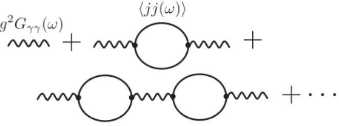
One first attempt to do so might involve summing the series of diagrams shown in Fig. 2. The geometric sum leads to an answer of the schematic form
hEEðωÞi∼ −ð−iωÞ2 g 2G
γγðωÞ
1−hjeljelðωÞig2GγγðωÞ
; ð3:31Þ
whereGγγ is the free photon propagator for spatial polar-izations and hjeljeli is the correlation function of the electrical current. The photon propagator at zero spatial momentum has a pole at ω→0; at low frequencies, we now zoom in on this pole to find for the resistivity r,
r∼ð−iωÞ 1 hjeljelðωÞi
∼1
σ; ð3:32Þ
where we have used the standard Kubo formula for the 0-form global conductivity hjeljelðω→0Þi ¼−iωσ. Thus, within this approximation scheme, it is indeed true that the resistivity (defined via our Kubo formula) is equal to the inverse of the conductivity of the current that is being gauged.9
Note, however, that this class of diagrams isnotthe only set of diagrams that one should include. One might also imagine diagrams of the form Fig. 3; computationally, they arise from the fact that the photon is now dynamical, and thus the classification of diagrams as “ one-particle-irreducible”has changed. Such diagrams will contribute to
(3.23); as they simply do not exist in the theory of the global 1-form currentjel, they will necessarily modify the
conclusion above, changingraway fromσ−1. We have not attempted a systematic study of such diagrams, but it would be very interesting to understand their effect. It seems likely that they can be suppressed at weak gauge coupling, justifying the approximation scheme above, but it is an important open issue to demonstrate precisely when this is possible.
IV. APPLICATION: DISSIPATIVE ALFVÉN AND MAGNETOSONIC WAVES
In this section, we study the collective modes of the relativistic MHD theory constructed above. We will linearly perturb the background solution and determine the dispersion relations ωðkÞ of the resulting modes. We organize the fluctuations in the following way: without loss of generality, we fix the direction of the background magnetic field by setting the hμ field to point in the z-direction, hμ¼ ð0;0;0;1Þ (note that its size is fixed by the normalization of hμ). Furthermore, we can use a residualSOð2Þsymmetry to fix the 4-momentum as
kμ¼ ðω; q;0; kÞ≡ðω;κsinθ;0;κcosθÞ; ð4:1Þ
so thatθmeasures the angle between the direction of the background magnetic field and momentum of the hydro-dynamic waves. The background velocity field is fixed to uμ¼ ð1;0;0;0Þ at rest, and the background temperature and chemical potential are kept general and space-time independent. We then linearly perturbuμ, hμ,T, andμas FIG. 2. Sum over current-current insertions to compute elec-trical resistivity.
FIG. 3. Example of new diagram that contributes to electrical resistivity.
uμ→uμþδuμe−iωtþiqxþikz; ð4:2Þ
hμ→hμþδhμe−iωtþiqxþikz; ð4:3Þ
T→TþδTe−iωtþiqxþikz; ð4:4Þ
μ→μþδμe−iωtþiqxþikz: ð4:5Þ
Note that linearized constraints (2.14)impose that
uμδuμ¼0; hμδhμ¼0; uμδhμþhμδuμ¼0: ð4:6Þ
For a background source without curvature, i.e.Hμρσ¼0, the fluctuations can be organized into two classes:
(i) Transverse Alfvén waves with
hμδuμ¼uμδhμ¼0; ð4:7Þ
kμδuμ¼kμδhμ¼0; ð4:8Þ
δT¼δμ¼0: ð4:9Þ
Note that the fluid displacement is perpendicular to the background magnetic field; thus, these waves can be thought of as the usual vibrational modes that travel down a string with tension. These modes were first discovered in the magnetohydrodynamic con-text by Alfvén in Ref. [39]. For an introductory treatment, see e.g. Ref. [40].
(ii) Magnetosonic waves withδuμandδhμcontained in the space spanned by fuμ; hμ; kμg. These are more closely related to the usual sound mode in a finite-temperature plasma. We will see that there are two branches of this kind: “fast” and“slow.”
We first study Alfvén waves. Solving the conservation Eqs. (2.4) and (2.5), we find the dispersion relation for Alfvén waves to Oðκ2Þto be
ω¼ vAκ−
i 2
1
εþpðη⊥sin 2θþη
∥cos2θÞ
þμ
ρðr⊥cos2θþr∥sin2θÞ
κ2; ð4:10Þ
where the parameter that enters the Alfvén phase velocity is
v2A¼V2Acos2θ; V2A¼ μρ
εþp: ð4:11Þ
The expression for the speed of the wave is standard. Recall thatμρis the tension in the field lines; in the nonrelativistic limit, (εþp) is dominated by the rest mass, and this becomes the textbook formula for the speed of wave propagation down a string. We are not, however, aware
of much previous discussion of dissipative corrections to Alfvén waves; Ref.[41]studied a dissipative fluid pertur-batively coupled to electrodynamics, and our expression reduces to their angle-independent result if we assume an isotropic shear viscosity and no resistivity.
When the magnetic field is perpendicular to the direc-tion of momentum, i.e. cos2θ¼0, the Alfvén wave ceases to propagate and becomes entirely diffusive, as is usually the case for transverse excitations in standard hydro-dynamics. Note that the width of the mode depends on the momentum perpendicular to the strings; elementary treat-ments of MHD often assume that the Alfvén wave has no dependence on the perpendicular momentum at all, which is sometimes taken as license to make it arbitrarily high, allowing Alfvén waves that are arbitrarily well localized in the plane perpendicular to the field (see e.g. Ref.[40]). Here, we see that this is an artifact of the ideal hydro-dynamic limit.
Turning now to the magnetosonic waves, a straightfor-ward but somewhat tedious calculation shows that the dispersion relations for the two magnetosonic waves are given by
ω¼ vMκ−iτκ2; ð4:12Þ
where
v2M¼1
2fðV2AþV20Þcos2θþV2Ssin2θ
ffiffiffiffiffiffiffiffiffiffiffiffiffiffiffiffiffiffiffiffiffiffiffiffiffiffiffiffiffiffiffiffiffiffiffiffiffiffiffiffiffiffiffiffiffiffiffiffiffiffiffiffiffiffiffiffiffiffiffiffiffiffiffiffiffiffiffiffiffiffiffiffiffiffiffiffiffiffiffiffiffiffiffiffiffiffiffiffiffi½ðV2
A−V20Þcos2θþV2Ssin2θ2þ4V4cos2θsin2θ
q
g: ð4:13Þ
Note that fast magnetosonic waves have aþsign before the square root in Eq. (4.13) and slow magnetosonic waves have a − sign. Above, we have defined the following quantities,
V2 0¼
sχ
Tðcχ−λ2Þ; ð4:14Þ
V2
S¼
s2χþρ2c−2ρsλ
ðcχ−λ2ÞðεþpÞ; ð4:15Þ
V4¼ sðρλ−sχÞ2
Tðcχ−λ2Þ2ðεþpÞ; ð4:16Þ
and the susceptibilities,
χ¼∂ρ
∂μ; c¼
∂s
∂T; λ¼ ∂s ∂μ¼
∂ρ
∂T: ð4:17Þ
Alfvén mode. We can interpretVSas the speed of the fast magetosonic mode atθ¼π2, a kind of speed of sound for the system. Atθ¼0, on the other hand, one magnetosonic mode has the same speed as the Alfvén mode, while the other one has velocity V0. We plot these velocities as a function of the angle θ for some interesting exam-ples below.
The dissipative parts of these modes can be calculated in a straightforward manner by going to one higher order in derivatives using the formalism above. Unfortunately, explicit expressions are rather cumbersome to write in print. We quote below only the values for τ at θ¼0 and θ¼π2, where we indicate which mode the width applies to by specifying the value of the phase velocity at that angle10:
τðVA;θ¼0Þ ¼1 2
η∥
εþpþ r⊥μ
ρ
; ð4:18Þ
τðV0;θ¼0Þ ¼21sTζ∥; ð4:19Þ
τ
0;θ¼π 2
¼1 2
η ∥ sTþ
r⊥ðεþpÞ2 T2ðs2χþρ2c−2ρsλÞ
; ð4:20Þ
τ
VS;θ¼π 2
¼1 2
ζ⊥þη⊥ εþp
þ r⊥ðcTρþρλμ−sTλ−sμχÞ2 T2ðcχ−λ2Þðs2χþρ2c−2ρsλÞ
:
ð4:21Þ
While the coefficient ζ× enters into the dispersion relations of magnetosonic waves, its coefficient is propor-tional to sin2θcos2θ, which implies that the magnetosonic dispersion relations have no dependence on the bulk viscosity ζ× at θ¼0 nor at θ¼π=2. Notice that the dissipative part (4.18) coincides exactly with the θ→0 limit of(4.10). This is expected, as in this limit there is an enhanced SOð2Þ rotational symmetry around the shared axis of background magnetic field and momentum, relating the modes in question. As a result of this coincidence, the results presented allow the measurement of only five of the seven dissipative coefficients. As it turns out, if we allow measurements at arbitrary angles, then ζ× can be deter-mined, but the value of η⊥ cannot be measured from the study of dissipation of linear modes alone. By introducing
sources, one can of course use the Kubo formulas pre-viously discussed to determine all transport coefficients.
A. Magnetohydrodynamics at weak field In order to recover the familiar results from standard magnetohydrodynamics, we can take the small chemical potential limit, which corresponds to weak magnetic fields. This is the regime in which the standard treatment is valid. In the weak-field limit, we can expand the equation of state as [cf.(2.26)]
pweakðμ; TÞ ¼p0ðTÞ þ 1
2g2ðTÞμ2þ ; ð4:22Þ
wherep0ðTÞandgðTÞare temperature-dependent functions that control the leading-order behavior. In this limit, to leading order,
v2A¼g 2μ2
sT cos
2θþ ; ð4:23Þ
ðv2
MÞfast¼ s
cTþ ; ð4:24Þ
ðv2
MÞslow¼ g2μ2
sT cos
2θþ : ð4:25Þ
This agrees with the standard treatment (for a relativistic discussion, see e.g. Ref. [41]). Notice that the slow magnetosonic mode and the Alfvén wave are indistinguish-able to this order. If we want to separate them, we need to go to higher order in the expansion. One nice example when one can do this and obtain concrete expressions is in the case whereμis much larger than any other scale in the problem (while still being much smaller thanT2). In this case, we have no other scale, and the expansion of the equation of state to the necessary order is
pweakðμ; TÞ ¼a 4T4þ
g2 2μ2þ
β
4
μ4
T4þ ; ð4:26Þ
wherea,g, andβare dimensionless constants. We find the leadingμ2 effects on the velocities of modes to be
v2A¼g 2μ2
aT4cos
2θþ ; ð4:27Þ
ðv2
MÞfast¼ 1 3þ
2 3
g2μ2 aT4sin
2θþ ; ð4:28Þ
ðv2
MÞslow¼ g2μ2
aT4cos
2θþ ; ð4:29Þ
v2A−ðv2MÞslow¼g 4þaβ
2a2
μ4 T8sin
22θþ : ð4:30Þ 10Note that, depending on the equation of state and the specific
values of μ and T (which determine the relative numerical magnitudes ofVA and V0), it can be either the fast or the slow
In each of the expressions, we have kept only the first nontrivial term to illustrate the angular dependence. The factor of 13in the leading-order expression for ðv2MÞfast is characteristic of the sound mode of conformal fluids in four dimensions. The fact that sound is the fastest mode is in agreement with our expectations at high temperatures where propagation is by nature diffusive. Note that both the Alfvén and the slow magnetosonic wave speeds start at
Oðμ2Þ, which is the small expansion parameter in this limit. Thus, they propagate very slowly indeed. We present some illustrative plots of these dispersion relations in Fig. 4(a).
B. Magnetohydrodynamics at strong field
The situation is quite different for a fluid in which magnetic fields are strong. Here, our formalism can make concrete predictions away from the weak coupling limit. For concreteness, let us assume, similarly as in the previous discussion, thatT2is much larger than any other scale in the problem, while still much smaller thanμ. In that case, we can write the equation of state in a small temperature expansion (strong magnetic field) as
pstrongðμ; TÞ ¼g 02
2 μ2þ a0
4T4þ
β0 8
T8
μ2þ ; ð4:31Þ
where g0, a0, and β0 are dimensionless constants. The expansion above is shown to the second subleading order to highlight that this expansion is, despite similarities, indeed different from(4.26). The fact that the leading-order terms agree (in form, but not numerical coefficients) between the two expansions is a coincidence due to our working in four dimensions.
From the above equation of state, we can calculate the mode velocities to first nontrivial order in temperature corrections:
v2A¼cos2θ−a 0T4
g02μ2cos
2θþ ; ð4:32Þ
ðv2
MÞfast¼1− a0T4 g02μ2
2
2þsin2θþ ; ð4:33Þ
ðv2
MÞslow¼ 1 3cos2θ
−T4cos2θ
9g02a0μ2
4g02β0þ3a 02sin2θ 2þsin2θ
þ :
ð4:34Þ
There are a few interesting features of these expressions. For propagation in the direction of the magnetic field lines, the Alfvén wave now has the same velocity as the fast magnetosonic mode, instead of having the same velocity as the slow mode, which was the case in the large temperature expansion. Furthermore, the speed of these modes is that of light in the strict T→0limit. This feature is completely general and independent of the particular no-scale assumption for the Alfvén wave. Another important differ-ence is that Alfvén modes can only propagate along magnetic field lines while fast magnetic modes propagate in any direction.
The slow magnetosonic mode is somewhat peculiar. Notice that theβ0coefficient contributes at an earlier order inTthan in the other modes. A more striking related feature is that the leading factor of13is not universal and depends strongly on the power of the leading temperature contri-bution. If, for example,a0 had been zero, we would have found that the zero-temperature velocity squared of the slow mode in the direction of the magnetic field lines was instead 17. Therefore, the high magnetic field limit is
0.1 0.2 0.3 0.4 V2
0.2 0.4 0.6 0.8 1.0V
2
(a) (b)
0.5 1.0 1.5 0.5 1.0 1.5
nonuniversal for this mode. The reason behind this is that this mode is the only one that contains δT fluctuations as
μ≫T2. It is an interesting question weather a universal hydrodynamic theory can be built that only describes the physics of fluctuating chemical potentials at fixed temper-ature ifμ≫T2. We answer this question in the affirmative in Sec. VI.
We present some representative plots of the velocities in the strong-field expansion in Fig. 4(b).
C. Cyclotron mode
Lastly, let us mention that by introducing a nontrivial curvature for the source of our generalized charge, we can recover the familiar cyclotron mode of plasma physics in the presence of a finite electric charge. At zero spatial momentum in the presence of a spatial and isotropic external field Hijk¼nϵijk, we find that the system can
undergo cyclotron motion with frequency
ω¼ 2n
μ ffiffiffiffiffiffiffiffiffiffiffiffi1þTs μρ
q : ð4:35Þ
V. MAGNETOHYDRODYNAMICS WITH A BARYON NUMBER
The theory that we have developed above demonstrates the essential physics in the hydrodynamics of conserved flux tubes. However, for phenomenological applications, we should extend it slightly to also include a conventional 0-form global symmetry (e.g. baryon number). This turns out to be entirely straightforward, and thus we present here only results without derivations.
We denote the baryon number current byBμ. We have ∇μBμ¼0, and we denote its conserved charge and
chemical potential by nB and μB. The thermodynamic
relations of interest are
εþp¼μBnBþμρþTs; ð5:1Þ
dp¼sdTþρdμþnBdμB: ð5:2Þ
At the level of ideal hydrodynamics, the relations
(2.12)remain unaltered, and the expression for the baryon current is
Bμð0Þ¼nBuμ: ð5:3Þ
The conservation equation forTμνis modified to include a contribution from an external gauge field FB¼dAB that
couples to the baryon current:
∇μTμν¼HνρσJρσþFνμBBμ: ð5:4Þ
Just as before, the ideal hydrodynamics equations result in a conserved entropy current suμ at the ideal hydrody-namic level.
If we move to first-order hydrodynamics, the canonical form for the entropy current is
Sμ¼suμ−1 TT
μν
ð1Þuν−μ
TJ
μν
ð1Þhν−μ
TB
μ
ð1Þ: ð5:5Þ
We expand the first-order correction to the baryon current as
Bμð1Þ ¼δnBuμþqhμþfμ; ð5:6Þ
withδnBandqfirst-order scalars andfμa transverse vector.
It is convenient to use scalar redefinitions of the baryon chemical potential to setδnB¼0; then, an entropy analysis
similar to that above results in the following expressions,
q¼−σ∥hμ
T∂μ
μB
T
−FB μνuν
; ð5:7Þ
fμ¼−σ⊥Δμν
T∂ν
μB
T
−FB νρuρ
; ð5:8Þ
where the transport coefficients σ⊥;∥ are simply conven-tional global (if anisotropic) conductivities for the baryon current.
VI. RELATIVISTIC MHD AT ZERO TEMPERATURE
In this section, we turn our attention to MHD at zero temperature. What do we mean by this? Normally, a system atT¼0is outside the hydrodynamic limit as there is no way to properly define a long wavelength limit compared with typical decay widths. Another way of stating this fact is the following: atT¼0, there is no dissipation, and this leads to long-lived excitations that do not arise necessarily as a consequence of conservation laws, leading to the presence of gapless modes that need to be included in the description of these systems. Also common is the presence of gapless Goldstone modes when there is a broken symmetry.
case, we are effectively studying a small part of the Hilbert space at energiesE∼μQ. In order to do this, we can then restrict to T¼0 in our equation of state and study the universal properties implied by the conservation of charge. Notice that an important feature of this system is that entropy is typically zero (i.e. the number of states we are considering is not exponentially large) according to the third law of thermodynamics. A curious counterexample to this seems to be holographic systems at finite density for standard conserved 1-form currents [42]. We will be agnostic about this for now and come back to this issue at the end of this section around Eq. (6.36).
The program above can be carried out in standard hydrodynamics of conserved 1-form currents. See Appendix B for a short discussion. The physics of this system is, however, conceptually not fundamentally differ-ent from usual hydrodynamics atT≠0. This is due to the fact that the symmetry breaking pattern of a system at finite density but with T¼0 is identical to that of the T ≠0 situation. It is always the case that the SOð3;1Þ Lorentz symmetry is broken down to SOð3Þ. This is because the charge density still selects a rest frame, even atT ¼0.
The situation is much more interesting in our description of magnetohydrodynamics. AtT ≠0andμ¼0, we have the usual symmetry breaking pattern SOð3;1Þ→SOð3Þ. At μ≠0, more symmetries are broken; the presence of background magnetic fields leads to the choice of a preferred spatial direction, further breaking Lorentz sym-metry as SOð3;1Þ→SOð2Þ and leading to the richer theory described in the previous sections. What happens atT¼0andμ≠0? Interestingly, the situation is different from the case discussed before. AtT¼0, there is only an antisymmetric tensor turned on in the background respon-sible for the magnetic field. This configuration is invariant under Lorentz boosts along the magnetic field lines. Therefore, in this case, we have an enhanced symmetry SOð3;1Þ→SOð1;1Þ×SOð2Þ with respect to the finite-temperature case.
This novel symmetry breaking pattern implies that the thermodynamic variables necessary to describe the system are completely different from the discussion in Sec.II. In what follows, we describe this new theory. There are concrete applications of this formalism in the understand-ing of systems at strong magnetic fields, such as some astrophysical systems.
A. Effective degrees of freedom
The relevant hydrodynamic fields are a scalar chemical potentialμand an antisymmetricuμνfield that parametrizes the rest frame enjoying SOð1;1Þ×SOð2Þ symmetry. We normalize it as
uμνuμν¼−2: ð6:1Þ As in usual hydrodynamics, the normalization is possible as
μcarries this information. What is crucial, however, is the
sign above, signalling that the tensor above is“mostly”in the plane acted on by SOð1;1Þ. This is similar to the familiar uμuμ¼−1 constraint. We would like, however, uμν to satisfy a stronger constraint and live entirely in the plane acted on by the SOð1;1Þ, so there exists a frame where the charge is entirely at rest. This is enforced in a covariant manner by further demanding that
uμνuνρuρσ¼uμσ: ð6:2Þ
It will be convenient to introduce a symmetric tensor,
Ωμν≡uμλu
λν: ð6:3Þ
The tensor Ω is the SOð1;1Þ-invariant metric on the 2D subspace spanned by the magnetic field. It projects any index onto this subspace. We will also make use of the projector orthogonal to this subspace, which projects onto theSOð2Þ-invariant sector,
Πμν≡gμν−Ωμν; ð6:4Þ
with traceΠμμ¼Ωμμ¼2. Henceforth, we will focus on the theory in flat space,gμν¼ημν. It will also be useful to visualize our construction in a Cartesian coordinate system aligned to the magnetic field by setting utz ¼−uzt ¼1, while all remaining components are zero. The SOð1;1Þ group then acts onðt; zÞand leaves invariant the metricΩμν. SOð2Þ acts onðx; yÞand leaves invariant the metric Πμν. We can now write down the most general stress-energy tensor and the antisymmetric conserved 2-form in flat space,
Tμνð0Þ¼−εΩμνþpΠμν; Jμνð0Þ¼ρuμν; ð6:5Þ
where ε, p, and ρ are functions of μ only. It is also important to note that the thermodynamic relation(2.19)
has now become
εþp¼μρ; dp¼ρdμ: ð6:6Þ
We can recover the zero temperature hydrodynamic theory of (6.5) from the finite-temperature theory (2.12)
by the following identification of the hydrodynamic var-iables,
uμν¼2u½μhν; ð6:7Þ
keepingμfinite and sendingTto zero. In this language, the symmetricSOð1;1Þand SOð2Þ metrics are
Ωμν¼hμhν−uμuν; ð6:8Þ
where Δμν is the finite-temperature projector from Eq. (2.15).
AtT2≪μ, we therefore expect a universal subsector of hydrodynamics to satisfy, in the ideal limit, the dynamical conservation equations
∇μTμνð0Þ¼0; ð6:10Þ
∇μJμνð0Þ¼0; ð6:11Þ
with the constituent relations(6.5).
As always, it is important to check that this system of equations closes and is not overdetermined. The system we are considering hasa priori5 degrees of freedom given by the scalarμand the 4 degrees of freedom inuμνsubject to the constraints(6.1)and(6.2). These 4 degrees of freedom can be viewed, in terms of symmetries, as the nontrivial action of the Lorentz group on a tensor preserving the SOð1;1Þ×SOð2Þsymmetries.
On the other hand, we see that the system above consists, naively, of eight equations of motion. This presents a danger, as the system of equations could be overdeter-mined. This is, however, not so. One of the equations (the time component of the charge conservation) is actually a constraint, as in the T ≠0 case. This constraint is con-sistently propagated by the other equations of motion. Thus, enforcing this constraint removes two equations of motion and 1 degree of freedom, still leaving an excess of two equations. For this system to not be overdetermined, they need to be trivial. Luckily, this is exactly the case for
(6.5). Consider the equation
ð∇μTμνÞΩνλþμð∇μJμνÞuνλ¼0: ð6:12Þ
This equality is satisfied off shell for any field uμν satisfying the constraints(6.1)and(6.2), and thus the two equations of motion that it contains are redundant. Therefore, the system of equations under consideration is consistent as a full set of nonlinear partial differential equations. Interestingly, as we elaborate in Appendix B,
Eq. (6.12) can be viewed as the natural zero-temperature
generalization of the equation for the conservation of the entropy current at finite temperature.
B. Beyond ideal hydrodynamics
We now move beyond ideal hydrodynamics. From the structure of available tensors, it is clear that there are no suitable one-derivative structures as they would have an odd number of indices. Therefore, Tμνð1Þ ¼Jμνð1Þ¼0. The leading-order corrections only enter at the level of second-order hydrodynamics. This observation, which follows only from available tensor structures is consistent with the fact that at T ¼0, the theory is expected to be nondissipative. Since first-order corrections to ideal
hydrodynamics are normally purely dissipative, such cor-rections should be absent.
To determine the form of the potential second-order corrections, we first discuss the decomposition of an arbitrary tensor under SOð2Þ×SOð1;1Þ. Using a; b;… for SOð1;1Þ indices and i; j;… for SOð2Þ indices, an antisymmetric tensorsμν breaks into three blocks:saband
sij, which are tensors underSOð1;1ÞandSOð2Þ,
respec-tively, as well as the off-diagonal elementssia that
trans-form as a product of vectors under SOð1;1Þ and SOð2Þ (denoted as v⊗v). A similar classification holds for symmetric tensors tμν, except that we can also extract out the scalar traces of the tensorstab andtij.
The three projectors onto the tensor representation of SOð1;1Þ,SOð2Þ, and vector representations ofSOð1;1Þ⊗ SOð2Þ are
SOð1;1Þ∶ PμνðωÞρσ¼ΩμρΩνσ; ð6:13Þ
SOð2Þ∶PμνðΠÞρσ ¼ΠμρΠνσ; ð6:14Þ
v⊗v∶PμνðvÞρσ¼ΩμρΠνσ þΠμρΩνσ; ð6:15Þ
with tracesPμðωÞμρσ¼Ωρσ,PμðΠÞμρσ¼Πρσ, andPμðvÞμρσ¼0. Hence, the symmetric and traceless projectors of an arbitrary matrixMμν onto the three sectors are
SOð1;1Þ∶
PððμνωÞÞρσ−1 2ΩμνΩρσ
Mρσ; ð6:16Þ
SOð2Þ∶
PððμνΠÞÞρσ−1 2ΠμνΠρσ
Mρσ; ð6:17Þ
v⊗v∶PððvμνÞρσÞ Mρσ; ð6:18Þ
and the antisymmetric parts follow fromP½μνρσMρσ in all three cases.
We now use this classification to parametrize the most general correction to(6.5), i.e. the analog of(3.3)at zero temperature:
Tμνð2Þ ¼−δεΩμνþδpΠμνþtSOμνð1;1ÞþtSOμνð2Þþtμνv⊗v;
Jμνð2Þ ¼δρuμνþsμνSOð2Þþsμνv⊗v: ð6:19Þ
Here, a two-index object with theSOð2Þor the SOð1;1Þ subscript indicates that the object transforms as a tensor under the appropriate group, whereas thev⊗v subscript indicates that it transforms as a product of vectors under SOð2ÞandSOð1;1Þ. Note that in the antisymmetric sector, any putative sμνSOð1;1Þ is proportional to uμν, and thus any corrections from those terms have been included in the