© 2017 Universidad Nacional Autónoma de México, Centro de Ciencias de la Atmósfera. This is an open access article under the CC BY-NC License (http://creativecommons.org/licenses/by-nc/4.0/).
Climatic analysis linked to land vegetation cover of Mexico by applying
multivariate statistical and clustering analysis
Luis F. PINEDA-MARTÍNEZ1* and Noel CARBAJAL2
1 Unidad Académica de Ciencias de la Tierra-PEIDA, Universidad Autónoma de Zacatecas, Calzada Universidad 108, 98058 Zacatecas, Zacatecas, México
2 Instituto Potosino de Investigación Científica y Tecnológica, A. C., San Luis Potosí, San Luis Potosí, México
*Corresponding author: email: [email protected]
Received: April 7, 2016; accepted: May 24, 2017
RESUMEN
Se delimitan las regiones climáticas de México mediante el análisis jerárquico de agrupamiento. Los datos utilizados fueron medias mensuales de temperatura máxima y mínima y la precipitación mensual acumulada, obtenidas de estaciones climáticas en México para el periodo 1961-2004. Este método de agrupamiento asigna cada variable de precipitación y temperatura a grupos con base en características estadísticas similares. Se realizó un análisis de componentes principales para obtener una matriz estandarizada que se utilizó en el agrupamiento. Aplicando dos criterios de agrupamiento (K-means y Ward) fue posible definir estadística-mente los grupos de estaciones que delimitan regiones de clima similar. Además, la metodología empleada describe la distribución de la vegetación dominante para cada región climática. Este análisis puede contribuir a la generación de nuevos escenarios climáticos, donde puede incluirse la dinámica de la cobertura vegetal como bioindicador del clima.
ABSTRACT
The climate regions of Mexico are delimitated using hierarchical clustering analysis (HCA). The data used consists of monthly means of maximum and minimum temperatures and monthly-accumulated precipitation. The dataset was obtained from heterogeneously distributed climatic stations in Mexico for the period from 1961 to 2004. This cluster method assigns precipitation and temperature variables to groups of clusters based on similar statistical characteristics. We carried out a principal components analysis to obtain a standardized reduced matrix to be used in HCA. By applying two clustering criteria (K-means and Ward´s method) it was possible to define statistically groups of stations that delimit regions of similar climate. In addition, the applied methodology describes the dominant vegetation distribution for each climate region. This analysis may contribute to the generation of new climate scenarios, where the dynamics of land vegetation cover could be included as a biomarker of climate.
1. Introduction
The relationship between climate and vegetation distribution has been used to make inferences about changes in the behavior patterns of both components. The classification of climatic regions can contribute to the knowledge about climate change and the
po-tential distribution of vegetation (Bonan et al., 2003).
There has been a climate typing attempt to introduce a series of rules in order to generate climatic region-alization based on the statistical analysis of long-term meteorological data. One of these statistical analyses, based on eigen techniques, represents an alternative that can be used to generate reproducible climatic maps (Richman, 1981). The climatology of Mexico has been described by some authors (García, 2004; Comrie and Glenn, 1998; Englehart and Douglas, 2002; Giddings et al., 2005, Bravo et al., 2012). However, for new methodologies to be introduced, it is indispensable to understand climatic zoning based on statistical data analysis. When defining climate regions, typically, long-term monthly means are employed from a set of climatic observations (tem-perature and precipitation) regarding a number of climatic stations (Pineda-Martínez et al., 2007). The principal aim of this research is to apply a hierarchical clustering analysis to historical meteorological data of Mexico.
Another aspect is the connection between cli-mate and vegetation. The distribution of potential global vegetation is entirely related to the climate and geographical conditions (Neilson, 1995;
Bonan et al., 2003). The estimation of vegetation
distribution in terms of climatic regions can be a useful tool for future approaches not only for the climate but also for the redistribution of potential vegetation under climate change scenarios. These interactions are key for understanding the water balance and its impact on the hydrological cycle
(Farmer et al., 2003).
The regions of native vegetation are adapted to contemporary climate conditions. As the climate changes every type of vegetation must change as well. The sites where climate becomes a factor of stress can cause changes in vegetation patterns and promote the invasion of exotic species (Cramer
and Leemans, 1993). This kind of alteration of the
vegetation cover may modify significantly the soil properties. The relationship between vegetation and
climate is essential to understand the interactions between the ability of the soil to store water and its impact on the processes of potential evaporation and precipitation.
This work aims to define climate regions for the whole territory of Mexico based on hierarchical clus-tering analysis from 2324 selected climatic stations. Cluster analysis is a useful tool to define groups of objects within a dataset based on similarity, thus it allows to define climatic regions. Also, we generate a classification of the main types of vegetation in each climatic region. The database of vegetation types used for this study corresponds to the nation-al forest inventory of 2000 (Pnation-alacio-Prieto et nation-al., 2000). Vegetation types are grouped by dominant vegetation type in representative groups (Miranda and Xolocotzi, 1963).
In this paper we generate a climatic regional-ization based on a robust statistical analysis. In the regionalization of climate we use vegetation cover as a guide to the discussion of the results. In this way, we focus on describing the main relationships between our climatic regionalization and vegetation patterns, and the topographic influence.
2. Data and methodology 2.1 Climate data
We use 2324 stations across Mexico’s territory (14º N, 86º W to 33º N, 118º W) for which the date record spans 40 years. The data was obtained from the Comisión Nacional del Agua (Mexican water commission), and it includes observations from sta-tions throughout Mexico (Fig. 1) (http://clicom-mex. cicese.mx).
For this research work, we consider monthly means of temperature maxima (January = T1 to December = T12), monthly means of temperature minima (January = t1 to December = t12) and monthly means of accumulated precipitation (P) (36 variables in total), for a period from 1961 to 2004. In order to obtain a matrix of average values, we included stations with continuous information during the considered period and those with no more than 2% missing data. Precipitation and temperature values were evaluated using quality controls similar to Zhu and Lettenmaier (2007). The variables were standardized to a 0 mean and a standard deviation
2.2 Principal components
The PCA was implemented as described in Gong and Richman (1995). The data matrix was used to compute the covariance between all variables or
entities (A). The data matrix X contains n stations
and m variables (2324 × 36). The n × m data matrix
yielded a m × m matrix. Since data were standardized
the resulting product matrix of the anomalies would be a standardized anomaly matrix, also known as a correlation matrix. As mentioned by Estrada et al. (2009), a correlation matrix is used to avoid that variables with larger magnitudes would dominate in the PCA results. The matrix was diagonalized into a
m × m matrix of eigenvalues and a matrix of
eigen-vectors. The eigenvectors were scaled by the square root of the corresponding eigenvalue. Once this was accomplished, some assessment of dimensionality
is often applied to reduce the m new variables (the
principal components) to a smaller set, r (Gong and
Richman, 1995). For this research, we retained the principal component with eigenvalue > 1.
The m × r matrix was transformed by a varimax
orthogonal rotation to obtain an m × r matrix of
rotated principal component loadings. From these
rotated loadings, an n × r set of principal component
scores are formed and a Euclidian distance measure is applied to those scores. The distances are used as inputs for the cluster analysis.
This PCA has the goal of replacing the correlated climatic original variables with new components,
which are mutually uncorrelated based on the princi-ple that each component is defined by an orthogonal basis (Richman, 1981). Thus, the eigenvector matrix resulting from this type of PCA is often truncated. retaining PC with eigenvalues ≥ 1 (Gong and Rich-man, 1995).
The entries of this matrix, the eigenvectors or loadings, define new variables, consisting of linear transformations of the original variables. Thus, PCA generates another matrix that represents new uncor-related variables (Richman, 1981).
2.3 Cluster analysis
Hierarchical cluster analysis (HCA) allocates a set of objects into groups or clusters on the basis of some measurement of similarity. This similarity or distance is an Euclidean measurement, i.e., it is a simple difference between two objects (Fovell and Fovell, 1993; Karlsen and Elvebakk, 2003).
Agglomerative cluster is an algorithm that starts
with n clusters, each containing one single object,
and then neighbor cluster pairs merge iteratively at each step to create new clusters (Elmore and Rich-man, 2001). Thus, the number of remaining clusters is reduced by one after every step and the procedure finishes when only one cluster containing all the ob-jects is created (Karlsen and Elvebakk, 2003).
In order to identify the minimum number of suit-able clusters, a K-means clustering was carried out to group the data based on similarity of PC’s. The
–115 30
25
(Latitude ºN
)
20
15
–110
(Longitud ºW)
Elevation (m) 3800 3500 3500 2900 2600 2300 2000 1700 1400 1100 800 500 200
–105 –100 –95 –90
K-means algorithm is a convergent method where
k seed points are specified as a set of centroids of k
clusters. The Euclidean distance is computed; then each entity is assigned to a cluster having the nearest centroid to attain an initial partition. The minimum cluster number is determined under a convergent
criterion by comparing the distances to all the k
clusters centroids.
Once a maximum number of clusters were ob-tained, we carried out an agglomerative hierarchical clustering using Ward’s method, which is an ag-glomerative hierarchical cluster method that merges cluster pairs with the smallest inter-cluster Euclidean distance. Ward’s method, the most frequently used for climatic classification (Kalkstein et al., 1987), uti-lizes inter-cluster minimum variance as the distance criterion for merging cluster pairs that show the mini-mum squared distance between centroids (Fovell and Fovell, 1993; De Gaetano, 1996). Ward’s algorithm was carried out for the retained components from the PCA to obtain a climatic regionalization (Kalkstein et al., 1987). Since our final goal is the delimitation of climatic regions, every cluster will be classified using the Köppen climate classification modified by García (2004).
2.4 Silhouette coefficient
In order to determine the minimum cluster, the sil-houette coefficient (SC) was computed. The method of silhouette coefficients combines both cohesion and separation (Tan et al., 2005).
In order to compute the silhouette coefficient for an individual point, a process that consists of the
following three steps is carried out: 1) for the ith
object, its average distance to all other objects in its
cluster ai’ is calculated; 2) for the ith object and any
cluster not containing the object, the average distance to all the objects in the given cluster is calculated;
the minimum value with respect to all clusters is bi;
and 3) for the ith object, the silhouette coefficient is
Si = (bi – Ui)/max(ai’ bi)’.
The value of the silhouette coefficient can vary between –1 and 1. A negative value is undesirable
be-cause it corresponds to a case in which Ui, the average
distance to points in the cluster, is greater than bi, the
minimum average distance to points in another cluster.
We want the silhouette coefficient to be positive (ai <
bi), and for ai to be as close to 0 as possible, since the
coefficient assumes its maximum value of 1 when Ui =
0. We can compute the average silhouette coefficient of
a cluster by simply taking the average of the silhouette coefficients of points belonging to the cluster.
3. Results and discussion 3.1 Principal component analysis
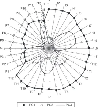
Figure 2 shows PC loadings for the three first com-ponents; it is possible to observe that all variables are grouped on different sectors. PCA results show a distribution of temperatures associated to the first principal component (PC1) and precipitation vari-ables associated to the second component (PC2). PC loadings are characterized by temperature variables through the PC1 with an explained variance of 52.9% and by precipitation variables through the PC2 with an explained variance of 19.2%. The first three prin-cipal components amounted to 82.1% of the total explained variance. Additional components had a lower effect on variance explanation (eigenvalue < 1).
As shown in Figure 2, monthly means of min-imum temperature had the highest contribution to PC1, revealing the large variability of this parameter.
1 t1 t2
PC1 PC2 PC3
t3 t4
t5 t6
t7
t8
t9
t10
t11
t12
T1 T2 T3 T4 T5 T6 T7 T8 T9 T10 T11 T12 P1 P2 P3 P4
P5 P6
P7 P8
P9 P10 P11
P12 0.8 0.6 0.4 0.2
–0.2 –0.4 –0.6 0
For instance, from an average temperature of 24 °C in warmer climates (state of Tabasco) to –4.25 ºC in colder ones (in the western Sierra Madre of Chihua-hua, see Fig. 1). It is reflected in major correlation values for these variables (from November to March). Maximum temperatures are associated with negative loadings in PC2 except from January to March. Less variability in temperature is observed through all data for spring and summer months. In contrast, PC3 shows an influence of summer temperatures and for precipitation in winter months.
3.2 Cluster analysis
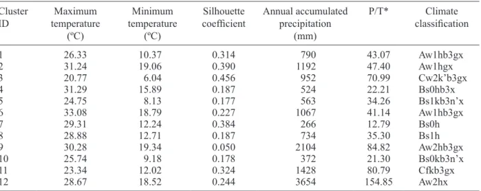
In order to generate the climate classification, it is necessary to delineate groups of stations which share similar meteorological characteristics. This delimitation was carried out by applying Ward’s agglomerative hierarchical clustering to the three first retained principal components. The spatial in-terpolation was done using a geostatistical ordinary kriging method and an exponential variogram in order to represent each cluster in its geographical context. Krigging was used to interpolate the position of the stations in the climatic groups. We used the cluster number assigned to each station after clus-tering. Once the interpolation was carried out, the climatic classification was performed for each clus-ter. Based on the results of the SC we examined the 12-level clustering solution (Table I).
The average silhouette coefficient is always posi-tive for all clusters, though some values are relaposi-tively low (close to 0) for specific groups of stations that present exceptional rainy climates (cluster 9). For these stations, grouped into clusters with larger SC values, the ranges of precipitation and temperature are low.
3.3 Climate regions classification
Clusters 4 and 5 reflect the semiarid climate regions (BSh and BSk) from the central part of Mexico north-wards (Chihuahuan Desert). These climates present low seasonal precipitation during summer due to a subtropical high-pressure zone and as a result of the geographical barriers of the main mountain ranges of Mexico. The difference between these two climates is the maximum temperature for the warm months (from May to July). Other arid zones that include the Sonoran Desert and the Baja California Peninsula were grouped in clusters 7 and 8 (BS0 and BS1). Despite their statistical similitude in terms of tem-perature values, cluster 7 clearly defined areas within the region delimited by cluster 8 with a difference in total precipitation and low precipitation/temperature (P/T) ratio.
The transition between the southernmost part of the highlands (2000 masl) and the area in which the western and eastern Sierra Madre converge in the central highland are defined in clusters 1, 2 and 9.
Table I. Characteristics of the clusters produced by clustering analysis. Cluster
ID temperature Maximum (ºC)
Minimum temperature
(ºC)
Silhouette
coefficient Annual accumulated precipitation (mm)
P/T* Climate
classification
1 26.33 10.37 0.314 790 43.07 Aw1hb3gx
2 31.24 19.06 0.390 1192 47.40 Aw1hgx
3 20.77 6.04 0.456 952 70.99 Cw2k’b3gx
4 31.29 15.89 0.187 524 22.21 Bs0hb3x
5 24.75 8.13 0.177 563 34.26 Bs1kb3n’x
6 33.08 18.79 0.227 1067 41.14 Aw1hb3gx
7 29.31 12.24 0.384 266 12.79 Bs0h
8 28.88 12.71 0.187 734 35.30 Bs1h
9 30.28 19.34 0.050 2104 84.82 Aw2hb3gx
10 25.74 9.18 0.178 372 21.30 Bs0kb3n’x
11 23.34 12.02 0.324 1428 80.79 Cfkb3gx
12 28.67 18.52 0.244 3654 154.85 Aw2hx
Cluster 9 (AW2) delimited the transition between temperate and humid climates near the Western Si-erra Madre. The wetter climate regions in the south-eastern part of Mexico were grouped in clusters 3 and 11 (Cwmh and Cfh) defining the humid and temperate climate regions. These regions are located in the coastal plains, in the Yucatán Peninsula and in the highlands of Chiapas. Cluster 11 (Cfh) delin-eated all of the central mountain formations from the western Sierra Madre to the lowlands (El Bajío) in the central part of Mexico. Overall, the Yucatán Peninsula and regions in the coastal zone of the Gulf of Mexico are contained in cluster 2 (Aw1), which thus defined the rainy climates. Cluster 1 (AW1b3) is located in the regions of tropical rainy forests with a seasonal precipitation regime and temperate climate. The rainiest climate regions are delimited by clusters 11 (Cfk) in Tabasco and the southeast of Chiapas, where usually tropical cyclones impact (García, 2004).
The P/T relation gives us an idea of the similitude between stations or groups. For instance, clusters 9 and 12 represent the same climate classification but under a different P/T regime. Thus, while cluster 9 has a P/T ratio of 84.82, for cluster 10 the ratio is 154.85. This means that large precipitations are most influenced by events such as tropical cyclones.
There are some implications for climate region-alization under global climate changes. Obviously, the present climates distribution will suffer changes for specific variables. In arid and semiarid regions in Mexico, the diurnal temperature oscillation has changed, mainly in its lower limits (Brito-Castillo et al., 2010). There is also a negative trend in soil moisture content from mid-latitude zones to the north-central region of Mexico, mainly due to low precipitation. This indicates a negative change in effective daily precipitation above 1 mm (Seager et al., 2007). These features needs to be considered in futures works on regional and local climate research.
3.4 Vegetation and climatic regions
Climate and topography control the distribution of many plants (Kelly and Goulden, 2008). Different species of plants have suffered some effects due to changes in temperature, especially during daytime. This has caused a variation in the species composition
in latitudinal and altitudinal gradients (Chen et al., 2011). Another important factor is the variation of drought periods that can affect the composition of species through the seed establishment of new individuals. In addition, areas of native vegetation have been modified and disturbed by the direct action of human activities. The intensification of these activities has impacted simultaneously with the changing climate conditions at a regional scale. In many cases, the vegetation groups include, at least partially, communities that cannot be catego-rized as climax, but its existence is largely linked to the characteristics of the substrate (Miranda and
Xolocotzi, 1963; Chapin et al., 2011). The present
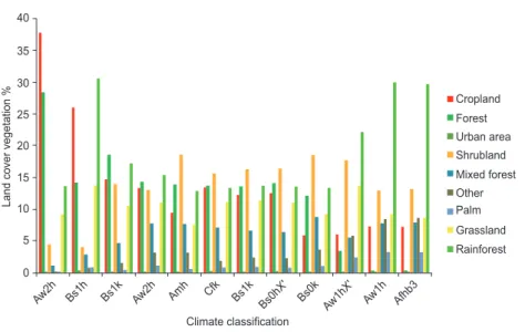
knowledge about land vegetation cover in Mexico does not allow comparative assessments in suffi-cient detail, except for specific sites and at a small scale (Rzedowski, 2006). Studies on vegetation are mainly focused on major vegetation types and they only show vegetation types as the basic unit of work. From the dynamic point of view, all vegetation types are described as stable biotic communities or plants based on the factors of the physical environment in which they live. For instance, although there are forests classified as secondary (mainly pine), others are the original plant or a mixture of both. Thus, vegetation types are grouped by dominant vegetation type in representative groups (Miranda and Xolocotzi, 1963). However, in this research work, we can infer reconstructions of the original vegetation. It is also possible to observe a relation-ship between the recent dominant vegetation and climate classification. This can be seen in Figure 3.
philos-Aw2h Bs1h Bs1k Aw2h Amh Cfk Bs1k Bs0hX Bs0k '
Aw1hX '
Aw1h Afhb3
Climate classification
Cropland Forest
Mixed forest Other Palm Grassland Rainforest Urban area Shrubland 40
35
25 30
20
15
10
Land cover vegetation
%
5
0
Fig. 3. Partial distributions of vegetation groups for climate type classification.
Fig. 4. (a) Climate regionalization types correspond to clustered regions; (b) Climate classification of Köppen modified by García (2004); (c) Stations grouped by cluster number; (d) Major vegetation groups in Mexico.
AC
Aw1hb3gr Aw2hb3gr Aw1hgx Aw1hx Bs0h Bs0hb3x Bs0kb3n'x Bs1kb3n'x C1kb3gx Cw2k'b3gx Bs1h
Climate
Climate
García (2994) ACf
Cf Cm Cmf Cs Cw EF ET
Cropland 1
(a) (b)
(c) (d)
Cluster 2 3 4 5 6 7 8 9 10 11 12
Mixed forest Rain forest Grassland Shrubland Palm Water bodies Other
ophies. While García (2004) includes geographic and topographic assessment criteria for boundary assignment, we base spatial boundary assignments on geostatistical techniques.
Figure 4d shows the cover vegetation; it is ob-served a pattern width of dominant crops in climates Bs and Aw, principally where rain-fed crops are established. Historically crops were established in rangelands of dominant grasslands landscapes.
Arid and semi-arid climates (type) B cover most of the Mexican territory from the northwest in the peninsula of Baja California, and especially in the central-north region. This region is defined by a geographic effect. The differences in altitude between the center highlands and the coastal plains result in a large climate mosaic and vegetation gra-dient. Furthermore, the arrangement of mountains directly influences the distribution of moisture and temperature ranges. These factors partially define the aridity of that region known as the Altiplano. The large proportion of continental land in the north part of Mexico is characterized by arid regions that limit areas of scrubland and grassland. Therefore, grasslands are widely distributed in these climatic regions, with precipitation conditions as the main driver, expressed in different representative spe-cies of grassland within each region. For example, semiarid grasslands of the Chihuahuan Desert can be distinguished in the semi-dry and cold climate BS0 and Bs1 groups.
The northwestern part of Mexico is significantly affected by a high-pressure cell for most of the year increasing the degree of aridity (Mosiño and García, 1973). Additionally, this region is directly influenced by a cold Pacific Ocean current that has a noticeable effect on the climate of the Baja California peninsula and of the state of Sonora, which drives the vegetation of this region, marked by the dominance of arid spiny shrubland distinctive of Bs0 climates. Shrublands are almost uniformly distributed throughout almost all of the climatic regions due to the large number of species and groups of shrubs found in Mexico. Nevertheless, it is possible to make a sub-classifi-cation of types of shrubland in correlation with the climatic classification in a gradient of moisture, from semi-desert scrubs in regions with annual average rainfall of 300 mm, to xeric scrub in regions with precipitation of 500-650 mm.
4. Conclusions
By applying techniques that include a combination of PCA and HCA, it was possible to carry out a fast clustering method based on the number of the princi-pal climate regions of Mexico; it allowed determining the maximum clusters number. By using the first three PC in the clustering method, the classification presented by multivariate techniques give a very close representation of previous regionalization work of García (2004).
The inclusion of the silhouette coefficient as a criterion to evaluate the clustering was very useful not only for grouping but also for determining the number of clusters. Therefore it was possible to determine a maximum number of clusters for hierarchical agglom-erative clustering algorithms. The Ward algorithm gives a better grouping using the silhouette coefficient as a criterion. In agglomerative clustering algorithms it is important to obtain an adequate number of clusters, which can be evaluated by means of the silhouette coefficient. Our results show mostly positive values for this coefficient, which tells us that the grouping criteria are adequate. Ward´s method is advantageous since it creates more homogeneous clusters from a covariance or correlation matrix.
This paper presents the results based on the correla-tion matrix, which delivered groups according to their variability. The importance of this regionalization for Mexico is that it provides the basis for further analysis on regional climate variations, according to their vul-nerability to climate change. The statistical techniques applied to the climatic database to generate a climate map show a high correspondence with the land cover map. By disaggregating station in groups, we can infer, in terms of the dominant vegetation, which of these regions will be more susceptible in its climatic structure under global climate variations.
Acknowledgments
This work was supported by the project SEP-CONA-CYT CB-2011-01- 168011. We thank Dr. Juan Gaviño Rodríguez for his comments on this manuscript.
References
simulated vegetation dynamics. Glob. Chang. Biol. 9, 1543-1566. DOI: 10.1046/j.1365-2486.2003.00681.x Bravo Cabrera J.L., E. Azpra Romero, V. Zarraluqui Such,
C. Gay García and F. Estrada Porrúa, 2012. Cluster analysis for validated climatology stations using pre-cipitation in Mexico. Atmósfera 25, 339-354.
Brito-Castillo L., E.R. Vivoni, D.J. Gochis, A. Filonov, I. Tereshchenko and C. Monzón, 2010. An anomaly in the occurrence of the month of maximum precipitation distribution in northwest Mexico. J. Arid Environ. 74, 531-539. DOI: 10.1016/j.jaridenv.2009.10.014 Chapin III F.S., P.A. Matson and P. Vitousek, 2011.
Princi-ples of terrestrial ecosystem ecology. Springer Science & Business Media, 455 pp.
Chen I.C., J.K. Hill, R. Ohlemüller, D.B. Roy and C.D. Thomas, 2011. Rapid range shifts of species associat-ed with high levels of climate warming. Science 333, 1024-1026. DOI: 10.1126/science.1206432
Comrie A.C. and E.C. Glenn, 1998. Principal compo-nents-based regionalization of precipitation regimes across the Southwest United States and Northern Mexico, with an application to monsoon precipitation variability. Clim. Res. 10, 201-215.
Cramer W.P. and R. Leemans, 1993. Assessing impacts of climate change on vegetation using climate clas-sification systems. In: Vegetation dynamics & global change (A.M. Solomon and H. Shugart, Eds.). Spring-er, 190-217 pp.
De Gaetano A.T., 1996. Delineation of mesoscale climate zones in the Northeastern United States using a novel approach to cluster analysis. J. Clim. 9, 1765-1782. DOI: 10.1175/1520-0442(1996)009<1765:DOMCZI>2.0. CO;2
Elmore K.L. and M.B. Richman, 2001. Euclidean distance as a similarity metric for principal compo-nent analysis. Mon. Wea. Rev. 129, 540-549. DOI: 10.1175/1520-0493(2001)129<0540:EDAASM>2.0. CO;2
Englehart P.J. and A.V. Douglas, 2002. Mexico’s sum-mer rainfall patterns. An analysis of regional modes and changes in their teleconnectivity. Atmósfera 15, 147-164.
Estrada F., A. Martínez-Arroyo, A. Fernández-Eguiarte, E. Luyando and C. Gay, 2009. Defining climate zones in Mexico City using multivariate analysis. Atmósfera 22, 175-193.
Farmer D., M. Sivapalan and C. Jothityangkoon, 2003. Cli-mate, soil, and vegetation controls upon the variability
of water balance in temperate and semiarid landscapes: Downward approach to water balance analysis. Water Resour. Res. 39, 1-21. DOI: 10.1029/2001WR000328 Fovell R.G. and M.Y.C. Fovell, 1993. Climate zones
of the conterminous United States defined us-ing cluster analysis. J. Clim. 6, 2103-2135. DOI: 10.1175/1520-0442(1993)006<2103:CZOTCU>2.0. CO;2
García E., 2004. Modificaciones al sistema de clasificación climática de Köppen, 5a. ed. Instituto de Geografía, UNAM, 90 pp.
Giddings L., M. Soto, B.M. Rutherford and A. Maarouf, 2005. Standardized precipitation index zones for Mex-ico. Atmósfera 18, 33-56.
Gong X. and M.B. Richman, 1995. On the application of cluster analysis to growing season precipitation data in North America east of the Rockies. J. Clim. 8, 897-931. DOI: 10.1175/1520-0442(1995)008<0897:OTAOC-A>2.0.CO;2
Kalkstein L.S., G. Tan and J.A. Skindlov, 1987. An evalu-ation of three clustering procedures for use in synoptic climatological classification. J. Clim. Appl. Meteorol. 26, 717-730.
DOI: 10.1175/1520-0450(1987)026<0717:AE-OTCP>2.0.CO;2
Karlsen S.R. and A. Elvebakk, 2003. A method using indicator plants to map locale climatic variation in the Kangerlussuaq/Scoresby Sund area, East Greenland. J. Biogeogr. 30, 1469-1491.
DOI: 10.1046/j.1365-2699.2003.00942.x
Kelly A.E. and M.L. Goulden, 2008. Rapid shifts in plant distribution with recent climate change. Proc. Natl. Acad. Sci. 105, 11823-11826. doi: 10.1073/pnas.0802891105 Miranda F. and E.H. Xolocotzi, 1963. Los tipos de
vegetación de México y su clasificación. Colegio de Postgraduados, Secretaría de Agricultura y Recursos Hidráulicos, Mexico,148 pp.
Mosiño A. and E. García. 1973. The climate of Mexico. In: Climates of North America, World Survey of Clima-tology 11 (R.A. Bysan and F.K. Hare, eds.). Elsevier, Amsterdam, 345-404.
Neilson R.P., 1995. A Model for predicting continen-tal-scale vegetation distribution and water balance. Ecol. Appl. 5,362-385.
DOI: 10.2307/1942028
México. Resultados del Inventario Forestal Nacional 2000. Investigaciones Geográficas 43, 183-203. Pineda-Martínez L.F., N. Carbajal and E. Medina-Roldán,
2007. Regionalization and classification of bioclimatic zones applying principal components analysis (PCA) in the central-northeastern region of México. Atmósfera 20, 111-222.
Rzedowski J., 2006. Relaciones geográficas y posibles orígenes de la flora. La vegetación de México. Comisión Nacional para el Conocimiento y Uso de la Biodiversidad, Mexico. Available at: . http://www. biodiversidad.gob.mx/publicaciones/librosDig/pdf/ VegetacionMx_Cont.pdf.
Richman M.B., 1981. Obliquely rotated principal com-ponents. An improved meteorological map typing technique? J. Clim. Appl. Meteorol. 20, 1145-1159.
Seager R., M. Ting, I. Held, Y. Kushnir, J. Lu, G. Vecchi, H.-P. Huang, N. Harnik, A. Leetmaa, N.-C. Lau, C. Li, J. Velez and N. Naik, 2007. Model projections of an imminent transition to a more arid climate in southwestern North America. Science 316, 1181-1184. DOI: 10.1126/science.1139601
Tan P.-N., M. Steinbach and V. Kumar, 2005. Cluster anal-ysis: Basic concepts and algorithms. In: Introduction to data mining (P. Tan et al., Eds.). Addison-Wesley, Boston, 487-568.
Zhu C. and D.P. Lettenmaier, 2007. Long-term climate and derived surface hydrology and energy flux data for Mexico: 1925–2004. J. Clim. 20, 1936-1946.