Generation of Multiple Turbulent Flow States for the
Simulations with Ensemble Averaging
Boris I. Krasnopolsky1
c
The Author 2018. This paper is published with open access at SuperFri.org
The paper deals with the problem of improving the performance of high-fidelity incompress-ible turbulent flow simulations on high performance computing systems. The ensemble averaging approach, combining averaging in time together with averaging over multiple ensembles, allows to speedup the corresponding simulations by increasing the computing intensity of the numerical method (flops per byte ratio). The current paper focuses on further improvement of the pro-posed computational methodology, and particularly, on the optimization of procedure to generate multiple independent turbulent flow states.
Keywords: Incompressible turbulent flow, Generalized sparse matrix vector multiplication, Multiple right-hand sides, Ensemble averaging.
Introduction
The high-fidelity simulations of turbulent flows for the complex geometries are among the typical applications for the high performance computing (HPC) systems. These applications are characterized by the high computational costs, long simulation times, and low computational efficiency, not exceeding several percent of the peak performance of HPC system. This leads to the situation when the simulations may take months to complete even using modern compute systems.
The present paper focuses on the problem of improving the performance and efficiency of the high-fidelity turbulent flow simulations. An approach to model incompressible turbulent flows, combining conventional time averaging with the ensemble averaging has been proposed in [1, 4]. This approach allows to parallelize the simulations in time and replace the single simulation with long time averaging by multiple simulations with much shorter time averaging intervals. The paper [4] suggests to perform each of these simulations independently and to obtain the simulation speedup by increasing the amount of utilized compute resources. This approach increases the corresponding computational costs for the simulation, but allows to speedup the calculations beyond the strong scalability limit. Alternatively, the paper [1] suggests to perform the simulations in a single run and rearrange the computations in order to utilize the operations with blocks of vectors. The multiple solutions of system of linear algebraic equations (SLAE) for the pressure Poisson equation can be combined in a single solution of SLAE with multiple right-hand sides (RHS). The memory traffic reduction when solving the SLAE with multiple RHS compared to multiple solutions of SLAE with single RHS vectors allows to increase the computational intensity of the algorithm (flops per byte ratio), and as a result, to speedup the turbulent flow simulations by a factor of 1.5–2.
Both simulation scenarios mentioned above are the limiting cases of the generalized algo-rithm, combining several independent runs and several flow states inside each run. The corre-sponding estimates and recommendations to choose the optimal simulation scenario have been proposed in [2].
While the results presented in [1, 4] demonstrate the proof of concept for the suggested approach to parallelize the simulations in time, several questions affecting overall simulation
speedup are not discussed in detail in these publications. Among them is the problem of gen-eration of multiple uncorrelated turbulent flow states to start averaging in time. The simplest approach used in the mentioned publications assumes the simulation of flow transition for mul-tiple different initial flow states. These calculations, however, produce significant computational overhead thus reducing the efficiency of the suggested methodology. The current paper focuses on the problem of improving the efficiency of the proposed ensemble averaging methodology, and particularly, on the aspects of efficient generation of multiple initial turbulent flow states. An alternative strategy to generate initial turbulent flow states based on introduction of random perturbations to the single flow state at different moments in time is examined. The efficiency of the methodology is analyzed in terms of the total time to compute m uncorrelated flow states, that can be used as initial flow states for time averaging.
The paper is organized as follows. Section 1 contains theoretical estimates reflecting the influence of generation of multiple turbulent flow states on the overall efficiency of the ensemble averaging methodology. A brief description of the computational codes used for the experimental evaluation is presented in Section 2. Section 3 is focused on the detailed description of the procedure used to generate multiple turbulent flow states and its experimental comparison with the basic one, including the full simulation of the transition interval for each of flow states. Finally, the Conclusion section concludes the paper.
1. Theoretical Estimates
The simplest, but computationally expensive way to generate multiple independent turbu-lent flow states comprises of modelling of transition to the turbulence for the flows with different initial states (e.g. laminar flows with different perturbations). The choice of different initial flow states guarantees the turbulent flow states finally to become uncorrelated. This statement is a result of exponential divergence of the turbulent flow trajectories in the phase state, and the corresponding divergence growth rate is determined by the Lyapunov exponent [6, 8].
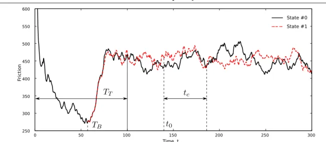
The corresponding simulation of transition to the turbulence for multiple flow states includes two characteristic time scales: (i) the time scale to perform transition to the statistically steady turbulent flow state, Tturb, and (ii) the decorrelation time scale when two different turbulent flow states become uncorrelated, Tcorr. The basic strategy to generate multiple turbulent flow states can be optimized depending on the ratio of these time scales. In case the transition time scale exceeds the decorrelation time scale, Tturb Tcorr, the procedure of generation multiple turbulent flow states can be obviously improved. For example, the simulation of the transition interval can be started for the single flow state. Then, the small perturbations are introduced at the bifurcation point, TB, to generate multiple uncorrelated flow states. The bifurcation point is reasonable to be chosen close to the end of the transition interval, TT, with the limitation TT −TB &Tcorr (Fig. 1).
The contribution of the optimized procedure to generate multiple turbulent flow states on the overall simulation speedup can be expressed with simple theoretical estimates. Let us consider the expected simulation speedup for the ensemble averaging approach with the suggested procedure to generate multiple initial flow states. Following the methodology suggested in [1], the simulation speedup Pm can be expressed as:
Pm = T1 Tm
Figure 1. Evolution of the friction at the channel walls for the problem of modelling turbulent flow in a channel with a matrix of wall-mounted cubes. Results are presented for two flow states; the second state is produced as a result of evolution of random perturbations introduced in TB moment in time
where T1 and Tm are the times to simulate the problem using averaging over single and m flow states respectively. The time to solve the problem with averaging over single flow state is expressed as:
T1 =
TT +TA
τ t1, (2)
where τ is the integration step, t1 is the time to simulate single integration step, and TA is the overall time averaging interval. The simulation time with multiple flow states includes the simulation with single flow state for the initial interval TB and the subsequent simulation of intervalTT −TB+TA/mwithm flow states:
Tm= TB
τ t1+
(TT −TB+TA/m)
τ tm. (3)
Here, tm is the time to simulate single integration step with m flow states. Substituting these expressions into (1) and introducing the parametersβ=TA/TT andγ = (TT −TB)/TT, one can obtain the following relation:
Pm =
1 +β
(1−γ) + (β+mγ)mt1
tm
−1. (4)
Using the estimate for the simulation times ratio based on the memory traffic reduction, proposed in [1], the final form of the estimate is obtained:
Pm=
5m(1 +β)
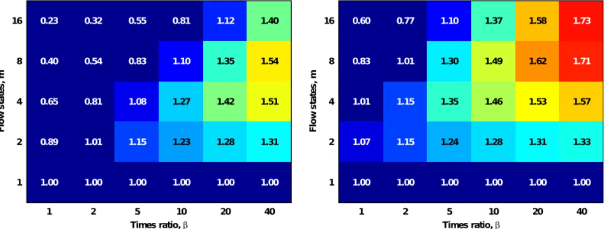
5m(1−γ) + (5m−3θ(m−1))(β+mγ). (5) The expression (5) is the generalization of the basic estimate in [1] on the case γ 6= 1.
multiple turbulent flow states leads to three major changes: (i) increase of the expected overall simulation speedup, (ii) increase of the optimal number of modelled turbulent flow states, and (iii) extension of the range of applicability for the proposed ensemble averaging methodology towardsβ ∼1.
Figure 2. Expected overall simulation speedup forγ = 1 (left) andγ = 0.25 (right)
2. Validation
The estimate (5) vividly demonstrate that reduction of computational costs to construct multiple independent flow states allows to significantly improve the range of applicability of the ensemble averaging methodology and the overall simulation speedup. The suggested approach to generate multiple turbulent flow states is based on fast decorrelation of different flow states compared to the transition interval. In practice, however, the length of both transition and decorrelation intervals is problem specific, and reliable estimates can only be obtained from some preliminary simulations.
2.1. Computational Codes
The corresponding computational codes to perform the simulations with multiple turbulent flow states, including the SLAE solver and “in-house” application for direct numerical simula-tion of turbulent flows have been developed. The SLAE solver implements the Krylov-subspace iterative methods, accelerated by the algebraic multigrid preconditioner. The “in-house” DNS code is based on finite difference scheme for structured grids [7] providing second-order spatial discretization together with third-order Runge-Kutta scheme for time integration. The further details on these codes can be found in [1, 3].
2.2. Test Problem
the kinematic viscosity of the fluid. The integration interval for this problem is set to T = 2100 with transition interval TT = 100 and averaging interval TA = 2000 time units, i.e. β = TA/TT = 20. The simulations presented in this paper are performed on structured orthogonal non-uniform computational grid consisting of 2.32 mln. cells. All the simulations are calculated on “Lomonosov-2” supercomputer and use 32 compute nodes per each run.
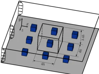
Figure 3. Sketch of the computational domain
2.3. Validation Procedure
The several simulations are performed to validate the procedure of generation multiple independent turbulent flow states with the introduction of random perturbations during the modelling of transition interval. The simulations differ in the choice of the bifurcation point. The cross-correlation functions are used to ensure the decorrelation of the corresponding flow states. The corresponding velocity components time series are collected in the control points around the cube. The cross-correlation function for two time series X and Y is defined as:
ρXY =
cov(X, Y)
var(X)var(Y), (6) where
cov(X, Y) = 1 tc
Z t0+tc
t0
(X(t)−X¯)(Y(t)−Y¯)dt,
¯ X = 1
tc
Z t0+tc
t0
X(t)dt, var(X) =cov(X, X).
The time series X and Y are the corresponding subsets of the velocity components profiles, defined by the starting pointt0 and the length of the intervaltc(Fig. 1).
3. Numerical Results
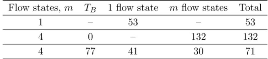
Initially, the simulation is performed with single flow state. Using the obtained intermediate data sets the simulation is restarted at TB = 77 to generate 4 decorrelated flow states. The corresponding simulation time, including the time to simulate single flow state over the interval TB and 4 flow states from the bifurcation point to the end of transition interval is equal to 71 min. (Tab. 1). This result indicates about 1.9 times speedup for the generation of multiple turbulent flow states compared to basic methodology where the perturbations are introduced at the beginning of transition interval.
Table 1.The time to generate multiple turbulent flow states with various simulation scenarios, results in min
Flow states,m TB 1 flow state m flow states Total
1 – 53 – 53
4 0 – 132 132
4 77 41 30 71
The second test series includes simulation of several full scale DNS runs to model flow over a matrix of wall mounted cubes. This includes the run with single flow state, the run with 4 flow states and two runs with restarts from the bifurcation point TB = 77 for 4 and 8 flow states. The corresponding compute times are summarized in Tab. 2. Using the expression (5) one can obtain the expected simulation speedup with the optimized procedure of generation multiple turbulent flow states compared to conventional DNS run. With basic procedure to generate initial turbulent flow states, the optimal number of flow states is equal to m= 4, and the speedup by a factor of 1.42 is expected. The obtained simulation speedup is 1.38, which is close to predicted one2. For the simulations with bifurcation point TB = 77, corresponding to γ = 0.23, performance gain for 4 flow states of about 1.53 is expected, and the optimal number of states is equal to 8 with the speedup by a factor of 1.63. These results correlate with the full scale simulation results, which are equal to 1.49 and 1.57 correspondingly.
Table 2.The computational times to simulate the turbulent flow with various number of simultaneously modelled flow states, results in min
Flow states,m 1 flow state m flow states Total
1 1088 – 1088
4 – 790 790
4 41 688 729
8 41 654 695
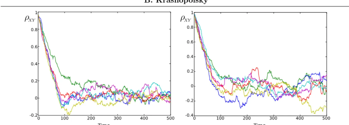
The time series for the velocity components monitored in 8 control points around the cube are analyzed to verify the obtained initial turbulent flow states are uncorrelated. The corre-sponding cross-correlation function distributions are evaluated for the time lengthtc= 100. The distributions presented in Fig. 4, demonstrate that the turbulent flows become uncorrelated before the end of transition interval, TT = 100.
2The presented simulation times obtained in the current test session are systematically 10-15% higher than the
Figure 4. Cross-correlation distributions for the streamwise velocity in different control points. Results for the simulation with 4 flow states
Conclusion
The current paper focuses on further improvement of the algorithm to model turbulent flows based on ensemble averaging, proposed earlier in [1]. The problem of reducing the compu-tational overhead when generating multiple initial turbulent flow states is investigated. The new procedure to generate uncorrelated flow states based on introduction of random perturbations during the modelling transition to the statistically steady turbulent flow state is proposed. The corresponding theoretical estimates demonstrate that the optimized procedure for generation multiple turbulent flows extends the range of applicability and improves the overall performance gain for the ensemble averaging approach. The corresponding numerical experiments performed for the problem of modelling the turbulent flow in a channel with a matrix of wall-mounted cubes are in agreement with suggested theoretical estimates and demonstrate additional 15% overall speedup for the ensemble averaging methodology.
Acknowledgements
The presented work is supported by the RSF grant No. 18-71-10075. The research is car-ried out using the equipment of the shared research facilities of HPC computing resources at Lomonosov Moscow State University.
This paper is distributed under the terms of the Creative Commons Attribution-Non Com-mercial 3.0 License which permits non-comCom-mercial use, reproduction and distribution of the work without further permission provided the original work is properly cited.
References
1. Krasnopolsky, B.: An approach for accelerating incompressible turbulent flow simulations based on simultaneous modelling of multiple ensembles. Computer Physics Communications 229, 8–19 (2018), DOI: 10.1016/j.cpc.2018.03.023
2. Krasnopolsky, B.: Optimal strategy for modelling turbulent flows with ensemble averaging on high performance computing systems. Lobachevskii Journal of Mathematics 39(4), 533–542 (2018), DOI: 10.1134/S199508021804008X
distributed systems with multicore CPUs and GPUs. In: Parallel Computing: On the Road to Exascale. Advances in Parallel Computing, vol. 27, pp. 93–102. Amsterdam, Netherlands (2016), DOI: 10.3233/978-1-61499-621-7-93
4. Makarashvili, V., Merzari, E., Obabko, A., Siegel, A., Fischer, P.: A performance analysis of ensemble averaging for high fidelity turbulence simulations at the strong scaling limit. Computer Physics Communications 219, 236–245 (2017), DOI: 10.1016/j.cpc.2017.05.023 5. Meinders, E., Hanjali´c, K.: Vortex structure and heat transfer in turbulent flow over a
wall-mounted matrix of cubes. International Journal of Heat and Fluid Flow 20(3), 255–267 (1999), DOI: 10.1016/S0142-727X(99)00016-8
6. Nastac, G., Labahn, J.W., Magri, L., Ihme, M.: Lyapunov exponent as a metric for assessing the dynamic content and predictability of large-eddy simulations. Physical Review Fluids 2(9), 094606 (Sep 2017), DOI: 10.1103/PhysRevFluids.2.094606
7. Nikitin, N.: Finite-difference method for incompressible Navier-Stokes equations in ar-bitrary orthogonal curvilinear coordinates. J. Comput. Phys. 217(2), 759–781 (2006), DOI: 10.1016/j.jcp.2006.01.036