Prediction intervals for characteristics of future normal sample under moving ranked set sampling

PREDICTION INTERVALS FOR CHARACTERISTICS OF FUTURE NORMAL SAMPLE UNDER MOVING RANKED SET SAMPLING

M. Al-Rawwash, M.T. Alodat, K.M. Aludaat, N. Odat, R. Muhaidat

1. INTRODUCTION

In a distinguished article aiming to estimate the population mean, (McIntyre, 1952) introduced a very clever idea for selecting a sample from the population of interest that appeared to be more representative than the Simple Random Sample (SRS) in carrying out the estimation process of the population mean. As a corner-stone in the literature of sampling theory, McIntyre’s work has been referred to as the Ranked Set Sampling (RSS). The motivation of RSS in applied fields arises in certain situations where ranking is considered to be easy compared to the high cost of the traditional sampling techniques. On the other hand, the handiness, flexibility and robustness of the RSS compared to its counterparts are considered additional advantages of the RSS scheme. Numerous articles and several books discussed the idea of RSS and its modifications over the last five decades (Taka-hasi and Wakimoto, 1968; Dell and Clutter, 1972; Martin et al., 1980; Kaur et al.., 1995; Muttlak, 1997; Alodat and Al-Saleh, 2001; Alodat et al., 2009, Alodat et al., 2010). To shed more light on the RSS approach, we describe the steps leading to an RSS of size m as follows. First we draw m independent random samples of size

m from the target population. Accordingly, using a visual inspection or any other cheap method, we detect the ith order statistic of the ith sample for actual quan-tification. The resulting quantified ordered statistics constitute an RSS of size m. Recently, the RSS technique has taken the attention of a large number of re-searchers in ecology, wildlife and agriculture where ranking units, using a visually inspection, has a negligible cost relative to their quantification. Despite the fact that perfect ranking is considered in this article, yet we conduct a pair wise com-parison between perfect and imperfect ranked set sampling and we elaborate on its importance during the course of this article.

(Chen, 2000). In fact, two factors may affect the efficiencies of estimators ob-tained via the RSS scheme namely, the set size (m) and the ranking error. (Al-Saleh and Alomari, 2002) showed that the larger the set size, the larger the effi-ciency of the estimator. On the other hand, increasing the set size, leads to tangi-ble difficulties in visual ranking of the sampled units. Carrying out the RSS pro-cedure may result in some kind of ranking errors. (Takahasi and Wakimoto, 1968) studied the performance of RSS when the ranking is perfect while ranking errors and its implications have been studied later by (Dell and Clutter, 1972). It has been shown that ranking errors do not affect the superiority of RSS over SRS while estimating the population mean as well as other vital parameters (Presnell and Bohn, 1999). On the other hand, the advantage of RSS will faint in the case of imperfect sampling and eventually if the ranking process is assumed to be completely random; it will yield equal variances using RSS and SRS techniques (Dell and Clutter, 1972; Cobby et al., 1985). Moreover, (Evans, 1967) noted that there is no practical difference between visual-type ranking and the actual detailed quantification of the units. For these reasons, modifications of RSS were pre-sented in the literature to study the effect of ranking errors that the experimenter makes (Alodat and Al-Saleh, 2001; Al-Saleh and Alomari, 2002; Samawi et al., 1996). Moreover, (Presnell and Bohn, 1999) pointed out some of the common errors presented in the RSS literature regarding perfect and imperfect ranking. They provided examples and counterexamples to show the possibility of obtain-ing more efficient results usobtain-ing imperfect rankobtain-ing. They provide some theoretical detailed work to support their claims.

(Alodat and Al-Saleh, 2001) introduced the moving ranked set sampling (MRSS) which can be described as follows:

1. Select m simple random samples of sizes 1, 2, ..., m, respectively.

2. From the jth sample, j  1, 2, , m quantify the _jth _{order statistic} af-ter detecting it via a visual inspection or any other crude method.

3. Repeat steps 1 and 2, but by quantifying the minimum i.e., the first order statistic from each sample.

4. The steps (1)-(3) could be repeated several times to increase the sample size for fixed m.

fu-ture sample is constructed in section 3 and 4 based on MRSS and SRS, respec-tively. In section 5, we conduct numerical comparisons between MRSS and RSS using the length of the prediction interval as our main comparison criterion. The ranking error effect is discussed in section 6. Finally, we provide an overview ap-plication to grassland biodiversity data set in section 7 and conclude our work in section 8.

2. NOTATION AND THEORETICAL SETUP

Let 1 1 1

1 2

{X_j , ,..., }X_j X_jj and 2 2 2

1 2

{X_j , ,..., }X_j X_jj , j  1, 2, , m be a collection of 2m random samples from _{N( , }2_{) and define}

1j

Y and Y2j

to be an MRSS sample such that 1 1 1

1j min{ j1, ,..., }j2 jj

Y  X X X and

2 2 2

2j min{ j1, ,..., }j2 jj

Y  X X X . Also, let ( ) x and ( ) x denote the density and the cumulative distribution functions of the standard normal distribution. The fundamentals of the order statistic theory indicate that the random variables Y1j and Y2j have the following distribution functions (Arnold et al., 1992)

1 ( ; , ) 1 1

1

j j

j

y

F y

y

  

 

 





  

   _{ } __ 

 

  _{ }

 

and

2j( ; , ) j

y

F y   

    

 _{ }

 ,

respectively, for j 1, 2, ,m. The corresponding probability density functions are

1

1j( ; , ) j

j y y

f y     

  



      

 _{   }

   

and

1

2j( ; , ) j

j y y

f y     

  



      

 _{   }

   ,

1 1

E(Y j) yf j( ; , )y   dy  Aj

 



_

where

1 ( ;0,1)

j j

A 

_

Similarly, we may obtain the expected value of Y_2j as follows

2 2

E(Y _j)  yf _j( ; , )y   dy  B_j 



_

where

2 ( ;0,1)

j j

B 

_

One may notice that the random variables Y1j and Y2j have the same dis-tribution when 0 implying that Bj  Aj for all j 1, 2, , m, (Arnold et

al., 1992).

3. PREDICTION INTERVALS USING MRSS

In this section, we focus our attention on developing prediction intervals for a new future observation as well as the sample mean and the extreme order statis-tics of a future sample under the normality assumption. To accomplish this mis-sion, we define S Y Y1( ,1 2,...,Ym) to be a statistic based on a future sample ob-tained from N( , 2) while X X1, 2,...,Xn represents an observed random sample from N( , 2). To derive the prediction interval of the statistic

1( ,1 2,..., m)

S Y Y Y , we define another ancillary statistic S S S3( , )1 2 , where S2 is only a function of X X1, 2,...,Xn. Since the distribution of S3 does not depend

on  and 2, then for a confidence level 112, we have

1 3 1 2 1 2 1 2

( ( , ) ) 1

P a S S S a   

where a₁ and a12 denote the 1001 and 100(12) quantiles of the

distribu-tion of S S S3( , )1 2 , respectively. A 100(112)% prediction interval of S1 can be obtained by solving the following inequality for S1:

1 3( , )1 2 1 2

Let _Y* _{be a new observation distributed as N( , }2_{) and consider the statistic} * 1 2 2 2 1 1 0.5( ) ( ) m ij i j

Y Y Y

F Y Y      



(2)

where 1 ₁

1 1 m j j Y Y m 





1 1 m j j Y Y m 





1 1 1 2 m ij i j Y Y

m  





data belongs to a location-scale family, we may write the random variable Yij as

ij ij

Y   Z , where Zij has the pdf ( ;0,1)f zij for i1, 2 and j 1, 2, ,m. Also, we may notice that the probability density function ( ;0,1)f zij does not de-pend on the parameters  and  which implies that the distribution of the sta-tistic (2) does not depend on μ and σ too. Hence, equation (2) may be written as

* *

1 2 1 2

2 2

2 2

1 1 1 1

*

1 2

2

2

1 1

0.5( ) 0.5( )

( ) ( ) 0.5( ) ( ) m m ij ij

i j i j

m ij i j

Y Y Y Z Z Z

Y Y Z Z

Z Z Z

Z Z                   _             







where 1 1

1 1 m j j Z Z m 





1 1 m j j Z Z m 





1 1 1 2 m ij i j Z Z

m  





N . Eventually, the distribution of the statistic F could be found via Monte Carlo simulation method.

Similarly and based on a given future sample say W W1, 2,...,Wn, we may define new statistics that correspond to the average (W), the minimum (W(1)) and the maximum (W( )n ) To elaborate more on this idea, we define the random variable

k k

W   V , for k 1, 2, , n which allows us to construct the following parameter-free distribution statistics:

1 2 2 2 1 1 0.5( ) ( ) m ij i j

V Z Z

(1) 1 2 2

2

1 1

0.5( )

( )

m ij i j

V Z Z

H

Z Z

 

 







,

and

( ) 1 2

2

2

1 1

0.5( )

( )

n m

ij i j

V Z Z

E

Z Z

 

 







Theorem 1. Suppose that we have an MRSS, say Yij, i1, 2 and j 1, 2, , m, then based on the previously listed variables and assumptions we have

1. A 100(1) prediction interval of _Y* _is

2 2

2 * 2

/2 1 /2

1 1 1 1

( ) ( )

m m

ij ij

i j i j

Y F Y Y Y Y F Y Y

   







.

2. A 100(1) prediction interval of W is

2 2

2 2

/2 1 /2

1 1 1 1

( ) ( )

m m

ij ij

i j i j

Y G Y Y W Y G Y Y

   







3. A 100(1) prediction interval of W(1) is

2 2

2 2

/2 (1) 1 /2

1 1 1 1

( ) ( )

m m

ij ij

i j i j

Y H Y Y W Y H Y Y

   







4. A 100(1) prediction interval of W_{( )n} is

2 2

2 2

/2 ( ) 1 /2

1 1 1 1

( ) ( )

m m

ij n ij

i j i j

Y E Y Y W Y E Y Y

   







Where F G H, ,  and E are the th quantiles of the random variables

, ,

Proof. The 100(1) prediction interval of _Y* _{will be derived using equations} (1) and (2) and assuming that that S3 F S, 1Y*, 2 1 2

2

Y Y

S   and

1 2 /2

   . Similar approaches allow us to conclude the results presented in parts 2, 3 and 4.

4. PREDICTION INTERVAL USING SRS

To better illustrate the performance of the MRSS in obtaining the prediction intervals and for the sake of comparing these results to those using SRS, we plan to derive the aforementioned prediction intervals using the SRS scheme. To carry out this mission, we assume that X X1, 2,...,X2m is a random sample of size 2m from N( , 2) and U U1, 2,...,Un is a future sample distributed as N( , 2). Once again we make use of the standardization of the random variable X_j as

j j

X   R , where R_j has a standard normal distribution. Accordingly, we may introduce the following variables that represent a parameter-free distribution statistics

a. To predict a new observation (U1), we define the random variable I as fol-lows

1

2 2

2 2

1 1

( ) ( )

m m

j j

j j

U X V R

I

X X R R

 

 

 

 





,

where 2

1 1 2

m j j

X X

m 





1 1 2

m j j

R R

m 





b. To predict the sample mean ( )U of a future sample of size n, we define the random variable J as follows

2 2

2 2

1 1

( ) ( )

m m

j j

j j

U X V R

J

X X R R

 

 

 

 





(1) (1)

2 2

2 2

1 1

( ) ( )

m m

j j

j j

U X V R

K

X X R R

 

 

 

 





d. Finally, to predict the maximum (U( )n ) of a future sample, we need to define the following random variable L

( ) ( )

2 2

2 2

1 1

( ) ( )

n n

m m

j j

j j

U X V R

L

X X R R

 

 

 

 





Theorem 2. Based on the SRS scheme and considering the random variables

, ,

I J K and L, we may construct the prediction intervals for U1, U, U(1) and

( )n

U as follows:

1. A 100(1) prediction interval for U1 is

2 2

2 2

/2 1 1 /2

1 1

( ) ( )

m m

j j

j j

X I X X U X I  X X

 







2. A 100(1) prediction interval for U is

2 2

2 2

/2 1 /2

1 1

( ) ( )

m m

j j

j j

X J X X U X J  X X

 







3. A 100(1) prediction interval for U(1) is

2 2

2 2

/2 (1) 1 /2

1 1

( ) ( )

m m

j j

j j

X K_ X X U X K_ X X

 







4. A 100(1) prediction interval for U_{( )n} is

2 2

2 2

/2 ( ) 1 /2

1 1

( ) ( )

m m

j n j

j j

X L_ X X U X L_ X X

 







where ,I J K ,  and L are the th quantiles of the random variables , ,I J K

TABLE 1

The upper and lower quantiles of F, G, H, E, I, J, K and Lwhen n5 and 0.05

m F G H E I J K L

2 -1.9702

1.9671 -1.1186 1.1296 -3.2073 0.2517 -0.2292 3.1208 -2.0723 2.1067 -1.2467 1.2218 -3.3517 0.3091 -0.2939 3.3427 5 -0.6259

0.6279 -0.3162 0.3133 -0.8699 0.0382 -0.0469 0.8557 0.8043 -.8089 -0.4144 0.4128 -1.1126 0.0716 -0.0813 1.1237 8 -0.4087

0.4044 -0.1945 0.1971 -0.5505 0.0194 -0.0222 0.5429 -0.5695 0.5658 -0.2813 0.2831 -0.7809 0.0418 -0.0438 0.7701 12 -0.2931

0.2879 -0.1339 0.1338 -0.3845 0.0128 -0.0118 0.3851 -0.4351 0.4459 -0.2140 0.2076 -0.5958 0.0217 -0.0289 0.6022

5. SIMULATION STUDY

To compare the MRSS prediction intervals with the SRS prediction interval us-ing the aforementioned procedures, we use the expected lengths of the prediction intervals as a comparison criterion. To do so, we let T denote a random variable in the set {F, G, H, E, I, J, K, L} where T denotes the th quantile of the

ran-dom variable T. The results concerning the previously mentioned random vari-ables are presented in Tvari-ables 1 and 2 for different set size (m) and assuming the significance level  0.05. More precisely, Table 1 gives the lower and upper quantiles for n5 future samples while Table 2 presents these quantiles for

10

n future samples. The results of Tables 1 and 2 will be used to obtain the length of the prediction intervals using the two schemes, namely SRS and MRSS.

TABLE 2

The upper and lower quantiles of G, H, E, J, K and L when n10 and 0.05

m G H E J K L

2 -0.9659

0.9641 -3.7409 -0.0789 0.0872 3.7266 -1.0959 1.0962 -3.9786 -0.0604 0.0655 3.9673 5 -0.2516

0.2399 -0.9647 -0.1064 0.1035 0.9692 -0.3355 0.3361 -1.2662 -0.1049 0.1030 1.2548 8 -0.1485

0.1458 -0.6026 -0.0859 0.0859 0.6101 -0.2296 0.2129 -0.8534 -0.0963 0.0957 0.8615 12 -0.0999

0.0972 -0.4251 -0.0650 0.0667 0.4252 -0.1674 0.1572 -0.6479 -0.0858 0.0842 0.6550

To obtain the expected interval length, we need to define Q as follows

2

2

1

2

2

1 1

( ) , if SRS scheme is used,

( ) , if MRSS scheme is used.

m j j

m ij i j

X X

Q

Y Y



 



 

  

 _

 





Then the expected length of any interval has the form

1 /2 /2

It is possible to obtain E( )Q in a closed form in the case of SRS while the mission might not be feasible in MRSS case. As a result, we use simulation to ob-tain the values of the expected interval length. Since the normal distribution be-longs to the location scale family, then without loss of generality, we may assume

0

 and  1. Table 3 contains the expected length of the prediction intervals for SRS and MRSS for different values of m and n based on 5000 Monte-Carlo simulations. It can be seen from Table 3 that the MRSS intervals are shorter than the SRS intervals in terms of their expected length. Moreover, the larger the sam-ple size, the smaller the expected length.

TABLE 3

The expected interval length of prediction intervals when 0.05

n m F G H E I J K L

5 2 6.4590 3.6893 5.6793 5.4940 6.6891 3.9512 5.8596 5.8209 5 4.3635 2.1903 3.1603 3.1409 4.6997 2.4099 3.4501 3.5106 8 4.1074 1.9779 2.8790 2.8548 4.3165 2.1460 3.1278 3.0944 12 4.0220 1.8538 2.7504 2.7474 4.1770 1.9989 2.9246 2.9922

m

10 2 6.4590 3.1671 6.0069 5.9697 6.6891 3.5088 6.2716 6.2454 5 4.3635 1.7104 2.9867 3.0126 4.6997 1.9566 3.3833 3.3556 8 4.1074 1.4868 2.6099 2.6476 4.3165 1.6824 2.8796 2.9116 12 4.0220 1.3635 2.4924 2.4816 4.1770 1.5390 2.6654 2.7063

6. EFFECT OF RANKING ERRORS

In ranked set sampling, the resulting sample is obtained under the assumption that the error in personal judgment is absent. However, we can not ignore the ranking errors in an RSS sample. As mentioned in section 1, many authors have studied the effect of ranking errors on the efficiency of the RSS estimation ap-proach. To name a few, (Dell and Clutter, 1972; Stokes, 1976 and Nahhas et al.,

2004) proposed some models for visual ranking errors. In this section, we con-sider the model proposed by (Dell and Clutter, 1972) where they assumed that the _ith _{visual score for the i}th _{observation in RSS set is defined as}

i i i

V X  ,

where  ₁, ,...,₂ _n are independent and identically distributed as _{N(0, )}2



 inde-pendent of the X_i’s. To obtain an RSS sample with ranking errors, according to the additive model, we adopt the following steps:

1. Obtain Vi Xi i, where  1, ,...,2 n are independent and identically

2 (0, )

N _ .

2. Rank the Vi’s in an ascending order so that we may obtain

(1) ( 2) ... ( )n

V V  V . Also, let X[ ]i denote the value of X associated with the th

3. The values X_[1],X_{[ 2]},...,X_{[ ]n} represent an RSS sample with raking errors. TABLE 4

Values of E( )Q for different values of 2 

 and m

E( )Q

2





m With ranking errors Without ranking error

0.1 2 3 5 8 12

1.6217 2.3227 3.4766 5.0514 6.9109

1.6406 2.3017 3.4608 5.0560 6.91263 0.5 2

3 5 8 12

1.6229 2.2668 3.3814 4.8278 6.5332

1.6330 2.3016 3.4919 5.0492 6.9138 1.0 2

3 5 8 12

1.6281 2.2991 3.1270 4.4728 5.9191

1.6363 2.2992 3.4993 5.0554 6.9250

To obtain an MRSS with ranking errors, we adopt the above model and re-place n by j. Accordingly, we use the X[ ]j ’s in stead of X( )j ’s. Since T1/2 and T/2 are obtained from the exact distribution via simulation without ranking errors, then it is sufficient to make the comparison only based on the values of

E( )Q . Table 4 contains the values E( )Q for different values of 2



 and m. It can be clearly seen that the larger the value of 2



 , the larger the difference be-tween the two values of E( )Q . Also for small values of m, the difference be-tween the two values of E( )Q gets smaller.

To elaborate more on this idea, we highlight some of the recent work related to imperfect ranking errors. (Frey, 2007) proposed a model for imperfect ranking that assumed to be valid and flexible to cover a wide range of judgment ranking errors. On the other hand, (Presnell and Bohn, 1999) have considered the model of (Dell and Clutter, 1972) in addition to an artificial model for judgment ranking error. As an illustration, they showed that the imperfect ranking has asymptotic efficiency of 8/3 relative to perfect ranking if their judgment ranking is consid-ered such that

2 1

1

1, | 0.5| | 0.5|

2, otherwise

X X

J     



where X₁ and X₂ are identical and independently distributed as (0,1)U and

1 1

see that the numerical results are comparable for small values of 2



 and they are not far away when 2



 is large. It is important to note that small values of 2



 imply more accurate ranking, while large values of 2



 imply more ranking errors. According to these studies in addition to the findings of this article, we may conclude that the imperfect ranking may have positive or negative effect on esti-mation accuracy depending on the model that is considered for judgment ranking errors. For this, the numerical results presented in this section lie among the find-ings of (Presnell and Bohn, 1999) and therefore we expect to have an effect on the expected length of the prediction intervals due to ranking errors.

7. APPLICATION TO GRASSLAND BIODIVERSITY DATA

Since the introduction of the RSS concept by (McIntyre, 1952), the idea has re-ceived an extensive attention due to its tremendous valuable applications in ap-plied fields including but not limited to engineering, communications and ecology (Patil, 1995). For example, (Halls and Dell, 1966) utilized the RSS technique to estimate the weights of browse and herbage in a pine-hardwood forest of east Texas. They concluded that RSS is more efficient than SRS. Similarly, RSS was found to be more robust when applied for estimating the shrub phytomass in fo-rest stands (Martin et al., 1980). Further applications of RSS can be found in (Ev-ans, 1967 and Cobby et al., 1985).

30 25 20 15 10 20

15

10

5

0

Number of Species

Fr

e

q

ue

nc

y

Mean 20.46 StDev 5.841 N 78 Histogram (with Normal Curve) of Noumber of Species

40 30 20 10 0

99.9

99

95 90 80 70 60 50 40 30 20 10 5

1

0.1

Number of Species

Perc

e

n

t

Mean 20.46 StDev 5.841

N 78

KS 0.043 P-Value >0.150

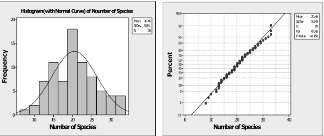
Figure 1 – Histogram with normal curve and normal probability plot for the number of species data.

precipi-tation varies between 950 and 1099 mm (Perner et al., 2005). The studied plant communities located between 11.018º and 11.638º eastern longitudes and be-tween 50.358º and 50.578º northern latitudes comprising a total of one hectare. We used grassland biodiversity in 78 sites. The data set was considered by (Alodat

et al., 2011) for estimating the mean and the standard deviation using MRSS. The histogram and the normal probability plot are given in figure 1. The histogram suggests a normal distribution while the normal probability plot shows a p-value larger than 0.15. So, the data provides us with no evidence to reject the normality assumption. In this section, we apply the MRSS procedure to the 78 observations and we divide the first 35 observations into 7 sets of sizes 2, 3,…, 8, and the last 35 observations into 7 sets of sizes 2, 3, …,8. Our plan is carried out by selecting the minimum of each set in the first group while we selected the maximum of e-ach set in the second group (see table 5).

TABLE 5

Illustration of MRSS for the Grassland Biodiversity

Group Set Minimum Maximum

1. {9, 21} 9

{15, 22, 17} 15

{18, 17, 19, 19} 17

{8, 33, 22, 33, 23} 8

{23, 19, 20, 19, 17, 12} 12

{18, 23, 26, 24, 13, 10, 15} 10

{23, 13, 22, 13, 19, 16, 21, 24} 13

2. {22, 13} 22

{16, 22, 31} 31

{23, 14, 13, 19} 23

{16, 22, 20, 18, 21} 22

{20, 25, 30, 28, 21, 27} 30

{25, 14, 28, 33, 20, 22, 21} 33

{27, 25, 27, 29, 26, 14, 25, 32} 32

TABLE 6

Prediction intervals for species data using SRS and MRSS

Statistic Prediction Interval Length

F (4.8092, 34.6155) 29.8063

G (12.4632, 26.9784) 14.5153

H (-0.33706, 20.2945) 20.6315

E (18.6707, 40.2393) 21.5686

I (3.60571, 35.655) 32.0493

J (11.6388, 35.655) 24.0162

K (-2.71866, 20.8626) 23.5812

L (18.5213, 41.1684) 22.6471

8. CONCLUSIONS

In this paper, we considered the problem of constructing classical prediction intervals for new observation, mean, minimum and maximum of a future sample from the normal distribution under the MRSS scheme. In terms of the interval expected length, we produced prediction intervals that are shorter than those ob-tained via the SRS scheme. This kind of prediction can be easily extended to other distribution families. Moreover, prediction intervals concerning characteris-tics of a future sample obtained via different ranked set sampling schemes could be considered. So we leave this to future research.

ACKNOWLEDGMENT

We would like to thank the referee for the valuable comments that helped us to im-prove the content of this article.

Department of Statistics, MOHAMMAD AL-RAWWASH Yarmouk University, Jordan

[email protected]

Department of Statistics, MOH’D ALODAT Yarmouk University, Jordan

[email protected]

Department of Statistics, KHALED ALUDAAT Yarmouk University, Jordan

[email protected]

Department of Biological Sciences, NIDAL ALODAT Al-Hussein Bin Talal University, Jordan

[email protected]

Department of Biological Sciences, RIYAD MUHAIDAT Yarmouk University, Jordan,

REFERENCES

M. T. ALODAT, K. M. ALUDAAT, N. ODAT, R. MUHAIDAT (2011), Parameters estimation of normal popu-lation via moving ranked set sampling with application to grassland biodiversity. Submitted.

M. T. ALODAT, M. Y. AL-RAWWASH, I. M. NAWAJAH (2010), Analysis of simple linear regression model via ranked set sampling, “Communications in Statistics-Theory and Methods”, 39(14), 2604-2616.

M. T. ALODAT, M. Y. AL-RAWWASH, I. M. NAWAJAH (2009), Analysis of simple linear regression via me-dian ranked set sampling, “METRON - International Journal of Statistics”, vol. LXVII, n. 1, pp. 1-18.

M. T. ALODAT, M. F. AL-SALEH (2001), Variation of ranked set sampling, “Journal of Applied

Sta-tistical Sciences”, 10, 137-146.

M. F. AL-SALEH, S. A. AL-HADRAMI (2003), Parametric estimation for the location parameter for symmet-ric distributions using moving extremes ranked set sampling with application to trees data, “Envi-ronmetrics”, 14(7), 651-664.

M. F. AL-SALEH, A. I. ALOMARI (2002), Multistage ranked set sampling, “Journal of Statistical

plan-ning and Inference”, 102, 273-286.

C. B. ARNOLD, N. BALAKRISHNAN, H. N. NAGARAJA (1992), A first course in order statistic,

John Wiley and Sons, Inc, New York.

Z. CHEN (2000), The efficiency of ranked-set sampling relative to simple random sampling under multi-parameter families, “Statistics Sinica”,10, 247-263.

J. M. COBBY, M. S. RIDOUT, P. J. BASSETT, R. V. LARGE (1985), An investigation into the use of ranked set sampling on grass and grass-clover swards, “Grass and Forage Science”, 40, 257, 263.

T. R. DELL, J. L. CLUTTER (1972), Ranked set sampling theory with order statistics background,

“Bio-metrics”, 28, 545-553.

M. J. EVANS (1967), Application of ranked set sampling to regeneration surveys in areas direct-seeded to longleaf pine, Masters Thesis, School of Forestry and Wildlife Management, Louisiana State University, Baton Rouge.

J. C. FREY (2007), New important rankings models for ranked set sampling, “Journal of Statistical

Planning and Inference”, 137, 1433-1445.

L. K. HALLS, T. R. DELL (1966), Trial of ranked set sampling for forage yields, “Forest Science”, 12,

22-26.

A. KAUR, G. P. PATIL, A. K. SINHA, C. TAILLIE (1995), Ranked set sampling: an annotated bibliography,

“Environmental Ecological Statistics”, 2, 25-54.

W. L. MARTIN, T. L. SHARK, R. G. ODERWALD, D. W. SMITH (1980), Evaluation of ranked set sampling for estimating shrub phytomass in Appalachian oak forest, Publication Number FWS-4-80, School of Forestry and Wildlife Resources, Virginia Polytechnic Institute and State University, Blacksburg, VA.

G. A. MCINTYRE (1952), A method of unbiased selective sampling using ranked sets, “Australian

Jour-nal of Agricultural Research”, 3, 385-390.

H. MUTTLAK (1997), Median ranked set sampling, “Journal of Applied Statistical Sciences”, 6.

245-255.

R. W. NAHHAS, D. A. WOLFE, H. CHEN (2004), Ranked set sampling: ranking error models and estima-tion of visual judgment error variance, “Biometrical Journal”, 46(2), 255-263.

G. P. PATIL (1995), Statistical ecology and related ecological statistics-25 years, “Environmental and

Ecological Statistics”, 2, 81-89.

J. PERNER, C. WYTRYKUSH, A. KAHMEN, N. BUCHMANN, I. EGERER, S. CREUTZBURG, N. ODAT, V. AU-DORFF, W. WEISSER (2005), Effects of plant diversity, plant productivity and habitat parameters on arthropod abundance in mountain European grasslands, “Ecography”, 28, 429-442.

B. PRESNELL, L. L. BOHN (1999), U-Statistics and imperfect ranking in ranked set sampling, “Journal

K. TAKAHASI, K. WAKIMOTO (1968), On unbiased estimates of the population mean based on the sample stratified by means of ordering. “Annals of the Institute of Statistical Mathematics”, 20, 1- 31.

H. M. SAMAWI, M. S. AHMAD, W. ABU-DAYYEH (1996), Estimating the population mean using ex-treme ranked set sampling, “The Biometrical Journal”, 38 (5), 577-586.

S. L. STOKES (1976), An investigation of the consequences of ranked set sampling, Ph.D. Thesis,

De-partment of Statistics, University of North Carolina, Chapel Hill.

SUMMARY

Prediction intervals for characteristics of future normal sample under moving ranked set sampling