Application of mathematical software in solving the problems of electricity

41

Application of mathematical software in

solving the problems of electricity

Erika Fechová

Technical University of Košice, Faculty of Manufacturing Technologies with a seat in Prešov, Bayerova 1,

080 01 Prešov, Slovakia [email protected]

Abstract

At the present time great emphasis is put on making accessible new knowledge to students through information and communication technologies in effort to facilitate and introduce objects, phenomena and reality. Information and communication technologies complement and develop traditional methods such as direct observation, manipulation with objects, experiment. It is justified mainly at teaching natural sciences. The possibilities of solving physical problem with the use of software tools are presented in the paper.

Keywords: information and communication technologies, electrical circuit, Kirchhoffov´s lows, MS Excel, Matlab.

doi: 10.23755/rm.v29i1.21

1 Introduction

42

it was several years ago. This gradually changes the style of teaching and makes teachers implement new technologies not only in direct pedagogical activity, but also at its preparation. Implementation of information and communication technologies into education enables new forms of university studies. We can stimulate the interest of students in studies of natural science subjects as mathematics, physics, chemistry, create conditions for educational individualization and improve conditions to raise the quality of education by a suitable combination of traditional and modern teaching methods [3].

In teaching physics there exist possibilities for effective and suitable integration of information and communication technologies into schooling system. One of them is physical problem solution with the support of computer. This paper concretely presents the solution of physical problem from the part Physics – Power and Magnetism by the use of mathematical software MS Excel a Matlab.

2 Physical analysis of the problem

Problem: Figure out the currents in individual circuit branches in Fig. 1, if source voltage and resistance are: U01=10 V, U02=20 V, U03=15 V, U04=10 V,

R1=10 , R2=15 , R3=30 , R4=20 , R5=10 , R6=15 , R7=10 .

Solution: Kirchhoff´s rules are used to figure out the currents in the circuit [4]. The first of Kirchhoff´s rules describes the law of electric charge preservation: The sum of all the currents flowing into the junction point must equal the sum of all the currents leaving the point, i.e.





 n

k k I 1

0. The second of

Kirchhoff´s rules forms the law of electric energy preservation for electric circuits: Algebraic sum of electromotive voltages in any closed part of the electrical network is equal to the sum of ohmic voltages at individual branches of this closed part, i.e.





 

 n k

k k m

i

ei R I U

1 1

43

Fig. 1.Circuit

Based on the first and the second of Kirchhoff´s rules (Fig. 1) for the currents and electromotive voltages, it is valid

0 0 0 7 6 5 3 5 4 3 2 3 2 1 1          I I I : B I I I : B I I I : B 0 4 0 3 7 7 6 6 0 3 6 6 5 5 4 4 0 2 4 4 3 3 2 2 0 2 0 1 2 2 1 1 U U I R I R : IV U I R I R I R : III U I R I R I R : II U U I R I R : I                

The set of 7 equations on 7 unknown quantities I1, I2, ..., I7 was obtained.

Numeric values are inducted for the known quantities and we have

5 10 15 15 15 10 20 20 20 30 15 10 15 10 0 0 0 7 6 6 5 4 4 3 2 2 1 7 6 5 5 4 3 3 2 1                         I I I I I I I I I I I I I I I I I I I

3 Analytic solution of the problem

Based on analysis of the problem and use of electrical laws the system of 7 equations in 7 variables was obtained, where analytic solution is not simple. In general it is possible to solve the system of n equations in n variables in three ways:

1. solving the system of linear equations by means of Cramer´s Rule, 2. solving the system of linear equations by means of inversion matrix, 3. solving the system of linear equations by Gauss elimination method.

44

The system of heterogeneous equations can be solved only if the rank of a matrix is equal to the rank of an augmented matrix of the system.

Consequence 1: If h(A)h(A)n (n is the number of unknowns), then the system has only one solution.

Consequence 2: If h(A)h(A)<n (n is the number of unknowns), then the system has infinite number of solutions and nh unknowns can be arbitrarily selected.

Consequence 3: If h(A)h(A), then the system has no solution.

We get the values of unknowns by gradual substitution into previous equations.

45                                                                                                                                                   110 530 0 15 0 20 0 2020 0 0 0 0 0 0 1060 1590 0 0 0 0 0 1 1 1 0 0 0 0 0 15 10 20 0 0 0 0 0 1 1 1 0 0 0 0 0 20 30 15 0 0 0 0 0 1 1 1 420 530 0 15 0 20 0 960 1590 0 0 0 0 0 1060 1590 0 0 0 0 0 1 1 1 0 0 0 0 0 15 10 20 0 0 0 0 0 1 1 1 0 0 0 0 0 20 30 15 0 0 0 0 0 1 1 1 10 10 5 0 15 0 20 0 0 0 0 0 0 15 10 10 15 0 0 0 0 0 1 1 1 0 0 0 0 0 15 10 20 0 0 0 0 0 1 1 1 0 0 0 0 0 20 30 15 0 0 0 0 0 1 1 1 5 15 20 10 0 0 0 10 15 0 0 0 0 0 0 15 10 20 0 0 0 0 0 0 20 30 15 0 0 0 0 0 0 15 10 1 1 1 0 0 0 0 0 0 1 1 1 0 0 0 0 0 0 1 1 1 6 1 R R 

The rank of a matrix is equal to the rank of an augmented matrix, i.e.

n h

h(A) (A) (n is the number of unknowns), then the system has one solution that is determined from an appropriate system:

05446 0 202

11 110

2020I7   I7  ,

46 24257 0 202 49 202 11 101 30 0 5 7 6 5 7 6 5 , I I I I I I I              40594 0 101 41 20 101 30 15 202 49 10 15 20 15 10 15 15 15 10 20 4 6 5 4 6 5 4 , I I I I I I I                               16337 0 202 33 202 49 101 41 0 3 5 4 3 5 4 3 , I I I I I I I                 46534 0 101 47 15 101 41 20 202 33 30 20 15 20 30 20 20 20 30 15 2 4 3 2 4 3 2 , I I I I I I I                              30198 0 202 61 202 33 101 47 0 1 3 2 1 3 2 1 , I I I I I I I                  

We get the following current values in the circuit:

A 05446 0 A 29703 0 A 24257 0 A 40594 0 A 16337 0 A 46534 0 A 30198 0 7 6 5 4 3 2 1 , I , I , I , I , I , I , I           

It results from the negative current values that currents in the circuit are in the opposite direction as we selected.

Analytic solution of the system of 7 equations in 7 variables by Gauss elimination method requires not only knowledge of linear algebra (matrix algebra), but also good mathematical skills and time. Numerical solution of the system of equations by means of various mathematical software tools such as MS Excel, Mathematica or MATLAB is much more easier.

4 Using software tools at the problem solution

47

In current computing technique it is possible to use standard programs for the matrix inversion up to relatively big number of equations (hundreds of variables). One of the possibilities is the solution in MS Excel [6]. We write the system of equations in matrix form

b

A 

    

 

   

 

    

 

   

 

   

 

   

 

x .

b b b

x x x

a a

a

a a

a

a a

a

n n n n n

n

n n

  

  

2 1 2 1

2 1

2 2 2

2 1

1 2 1

1 1

where A is the matrix of coefficients, x is the vector of unknowns and b is the vector of the second members. We get by multiplying A-1 from the left

b A A

A-1 xx -1 . If we calculate the inversion matrix, xk unknowns can be obtained by multiplication of the matrix and vector, which is procedure that is optimized very well and is the part of standard libraries of subprograms. To calculate the inversion matrix MINVERSE functions from the offer of MS Excel More Functions is used. To calculate the roots of the system of equations (A-1 b)

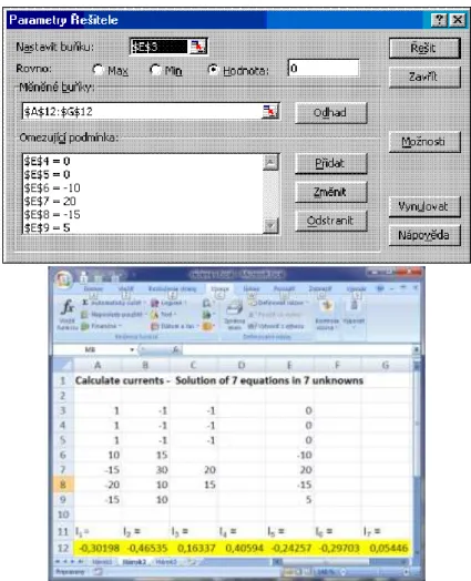
MMULT function is used. The result of the solution can be found in Fig. 2.

48

Fig. 3. Numerical solution of the system of problems in the MS Excel Solutionist

From both solutions in MS Excel we get the following current values in the circuit

A 05446 0 A

29703 0 A

24257 0

A 40594 0 A

16337 0 A

46535 0 A

30198 0

7 6

5

4 3

2 1

, I , ,

I , ,

I

, ,

I , ,

I , ,

I , ,

I

 

 



 

  



It results from the negative values of the current that currents have reverse directions as it was selected.

4.2 Problem solution by means of Matlab

49

[10]. The field is the basic data type of this interactive system. This property together with number of built-in functions enables relatively easy solution of many technical problems, mainly those that lead to the vector or matrix formulations, in much shorter time as solution in classic program languages. To calculate the currents I1, I2, ..., I7 the method of node voltage is used. This

method comes from the fact that (u1) equations is written by means of Kirchhoff´s first law applied to suitably selected nodes. In these equations the equations of Kirchhoff´s second law written for appropriate loops are implicitly included. That is why voltages on tree´s branches are selected as unknowns at the method of node voltage. To determine node voltages it is necessary to solve (u-1) equations. After calculation of node voltages the currents of the circuit are determined.

We write for B1, B2 and B3 nodes according to Kirchhoff´s first law

0 0 0 7 6 5 3 5 4 3 2 3 2 1 1          I I I : B I I I : B I I I : B

It is possible to express above mentioned currents by means of known node voltages with regard to the selected reference node

0 0 0 7 0 4 3 6 0 3 3 5 3 2 3 5 3 2 4 2 3 2 1 2 3 2 1 2 0 2 1 1 1 0 1 1                  R U U R U U R U U : B R U U R U R U U : B R U U R U U R U U : B B B B B B B B B B B B B B

We write the equations in the matrix form

                                           7 0 4 6 0 3 2 0 2 1 0 1 3 2 1 7 6 5 5 5 5 4 3 3 3 3 2 1 / / 0 / / / 1 / 1 / 1 / 1 0 / 1 ) / 1 / 1 / 1 ( / 1 0 / 1 / 1 / 1 / 1 R U R U R U R U U U U R R R R R R R R R R R R R B B B

50

Fig. 4. M-file prudy.m for calculation of matrices and currents

After solving the system of equations we get the values of node voltages, which are converted to the currents in branches of the circuit. The result of solution is launching the script of prudy.m and print of results.

51

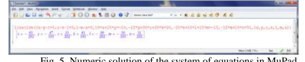
expressions. To solve the system of equations linsolve ([eqs], [vars]) function was used, where eqs is a list or a set of linear equations or arithmetical expressions, vars is a list or a set of unknowns to solve for: typically identifiers or indexed identifiers. The solution of the system can be found in Fig. 5, where x

= I1, y = I2, z = I3, k = I4, l = I5, m = I6, n = I7:

Fig. 5. Numeric solution of the system of equations in MuPad

The same values are obtained from the problem solution in Matlab as in the case of the problem solution in MS Excel.

5

Conclusions

It accrues from the solution results that solution of the system of equations of the physical problem in an analytic way as well as by using mathematical software tools leads to certain numeric values. Analytic solution of the system of

52

Bibliography

[1] Kalaš I. (2001) Čo ponúkajú informačné a komunikačné technológie iným

predmetom, ŠPÚ Bratislava

[2] Turek I. (1997) Zvyšovanie efektívnosti vyučovania, MC Bratislava

[3] Brestenská B. et al. (2010) Premena školy s využitím informačných

a komunikačných technológií, Elfa, s r. o Košice, ISBN 978-80-8086-143-8

[4] Bouche F. (1988) Principle of Physics. University of Dayton, ISBN 0-07-303579-3

[5] Kluvánek I., Mišík L., Švec M. (1971) Matematika I, Alfa Bratislava

[6] Brož M. (2004) Microsoft Excel 2003, Computer Press Brno, ISBN 80-251-0406-0

[7] Hrehová S., Mižáková J. (2008) Využitie MS Excel vo výpočtoch, Informatech, Košice, ISBN 978-80-88941-32-3

[8] Vagaská A. (2007) Matlab and MS Excel in education of numerical mathematics at technical universities, in: INFOTECH 2007, Votobia Olomouc

[9] Dušek F. (2002) MATLAB a SIMULINK, úvod do používaní, Univerzita Pardubice, ISBN 80-7194-273-1