Abstract—In this article, a synthesis approach for robust model predictive control using linear matrix inequalities is presented. Uncertain time-varying parameters and bounded additive disturbances are explicitly taken into account in the controller design. Robust stability and constraint satisfaction are guaranteed by computing a positively invariant set containing the measured state at each sampling instant. The effectiveness of the proposed algorithm is illustrated by a simulation example.
Index Terms—Robust model predictive control, uncertain time-varying parameters, bounded additive disturbances.
I. INTRODUCTION
Model predictive control (MPC) is an advanced control algorithm widely adopted in the chemical industry. At each sampling instant, a dynamic optimization problem based on an explicit process model is solved and the first computed input is implemented to the process. Since the process model is only an approximation of the real process, MPC should be robust to model uncertainty and disturbance [1]-[3].
Robust MPC synthesis of linear systems subject to uncertain time-varying parameters has been widely investigated [4]-[7]. The main idea is to compute an ellipsoidal invariant set that can guarantee robust stability of the closed-loop system. At each sampling time, a state feedback gain is obtained by solving an optimization problem subject to linear matrix inequality (LMI) constraints. Since only uncertain time-varying parameters are included in the MPC formulation, robust stability cannot be guaranteed in the presence of disturbances. Robust MPC synthesis using polyhedral invariant sets has also been widely studied [8]-[10]. In the problem formulation, it is assumed that there is no disturbance present so these algorithms cannot deal with disturbance.
In the context of tube-based robust MPC [11]-[13], disturbances are explicitly taken into account in the problem formulation. The main idea is to compute the regions around the nominal predicted trajectory that contain all possible states of the process. At each sampling time, a sequence of control inputs is obtained by solving an optimal control problem subject to constraints that are tighter than the original ones. Tube-based robust MPC can also handle model uncertainty if uncertain time-varying parameters are represented by virtual disturbances [14].
Manuscript received December 9, 2013; revised January 18, 2014. This work was financially supported by Mahidol University.
The authors are with the Department of Chemical Engineering, Faculty of Engineering, Mahidol University, Nakhon Pathom, Thailand (email: [email protected]).
Since there will always be model uncertainty and disturbance acting on the system, they should be considered in the controller design. In this paper, both uncertain time-varying parameter and bounded additive disturbance are explicitly taken into account in the MPC formulation. Robust stability and constraint satisfaction are guaranteed by computing a positively invariant set containing the measured state at each sampling instant. This article is organized as follows. In Section II, the problem statement is presented. In Section III, robust MPC synthesis is proposed. In Section IV, the effectiveness of the proposed MPC algorithm is illustrated by a simulation example. Finally, the conclusions are drawn in Section V.
Notation: For a vector x and a positive-definite matrix P,
Px x
xP2 T . x(k) is the state measured at real time k and
) /
(k i k
x is the state at prediction time ki predicted at real time k . The symbol denotes symmetric blocks in matrices. An element belonging to a convex hull Co
means that it is a convex combination of the elements in
.I is the identity matrix with appropriate dimension.
II. PROBLEM STATEMENT
Consider the following linear time-varying system
) ( ) (
) ( ) ( ) ( ) ( ) ( ) ( ) 1 (
k Cx k y
k v k D k u k B k x k A k
x
(1)
where nx
k
x( ) is the state, nu
k
u( ) is the control input, v
n k
v( ) is the disturbance and ny k
y( ) is the output. The superscripts nx , nu , nv and ny are the number of elements in x(k), u(k), v(k) and y(k), respectively. The input and output constraints are u(k)u ,
0
h
u ,h
1,2,...,nu
and Cx(k)y, yr0,r
1,2,...,ny
. It is assumed that any A(k) and B(k) belong to a convex polytope ΩABCo
[A1,B1],[A2,B2],..,[AnAB,BnAB]
and theycan be written as [ ( ), ( )] ( )[ , ]
1 j j
n
j j k A B k
B k
A
AB
,
1 ) (
1
AB
n
j j k where [Aj,Bj] are the vertices of ΩAB, nAB
is the number of [Aj,Bj] and j(k) are the uncertain
time-varying parameters. Any D(k) belongs to a convex
polytope
D
n
D CoD D D
Ω 1, 2,..., and it can be written as
Robust Model Predictive Control of Linear Time-Varying
Systems with Bounded Disturbances
t n
t t k D k
D D
1 ( )
)
( , ( ) 1
1
D
n
t t k where Dt are the
vertices of ΩD, nD is the number of Dt and t(k) are the
uncertain time-varying parameters. The disturbance v(k) is persistent, bounded and contained in a convex polytope
mv
v Cov v v
Ω 1, 2,..., where vs are the vertices of Ωv and v
m is the number of vs.
The objective of this research is to find a state feedback control law that is able to guarantee both robust stability and constraint satisfaction within a positively invariant set. The set Z is said to be positively invariant set if it has the property that whenever the current state is contained in this set
Z k
x( ) , all possible predicted states must be contained in this set x(ki/k)Z for all admissible realizations of
) (k i j
, t(ki) and v(ki), i0.
Consider the linear time-varying system (1) at each sampling time k , a state feedback control law
) / ( ) /
(k i k Kxk i k
u that (i) minimizes the upper bound
on J(k) and (ii) guarantees both robust stability and
constraint satisfaction within a positively invariant set
2
/ P
n x x
Z x where
P is a Lyapunov matrix, can be calculated by solving the following optimization problem
0
2 2
)] ( ), ( ,
, max ( ) [ ( / ) ( / ) ]
min
i n n
Ω i k B i k A P
K ABJ k x k i k Kx k i k
(2)
s.t. xn(ki1/k)[A(ki)B(ki)K]xn(ki/k) (3)
) ( ) ( ) / ( ] ) ( ) ( [ ) / 1
(k i k Ak i Bk iK xk i k Dk ivk i
x (4)
] ) / ( ) / ( [ ) / ( ) / 1
(k i k 2 x k i k 2 x k i k 2 Kx k i k 2
x n n
P n
P
n (5)
2
) (k P
x (6)
2
) / 1 (
P k i k
x (7)
u
h h n
u u k i k
Kx( / ) , 0, 1,2,..., (8)
y
r r n
y y k i k
Cx( 1/ ) , 0, 1,2,..., (9)
where xn(ki/k) is the predicted state not corrupted by
disturbances, and are symmetric weighting matrices. The cost monotonicity is guaranteed by (5). A positively invariant set containing the measured state at each sampling time is computed by (6). All possible predicted states are restricted to lie in a positively invariant set by (7). The input and output constraints are guaranteed by (8) and (9), respectively.
III. ROBUST MPCSYNTHESIS
Proposition 1: (The cost monotonicity) (5) and (6) are satisfied and the cost monotonicity is guaranteed if there
exists matrices Y, Q and a scalar such that the following LMIs are satisfied
0, {1,2,..., }
0 0 0
2 1 2 1
AB j
j
n j
I Y
I Q
Q Y B Q A
Q
(10)
0.
) (
1
Q k
x (11)
Then, it follows that is the upper bound on J(k).
Proof: By following [4], (5) and (6) are ensured by (10) and (11), respectively. By summing (5) from i0 to i and applying (6), it follows that J(k) .
Proposition 2: (Robust stability) (7) is satisfied if there exists matrices Y and Q such that the following LMIs are satisfied
AB
j j
n j
Q Y B Q A
Q
,..., 2 , 1 ,
0
(12)
2 21
) 1 ( , ,..., 2 , 1 , ,..., 2 , 1 ,
0
v D
s t
m s
n t
Q v
D (13)
where 01 is a pre-specified scalar. Then, all possible predicted states are restricted to lie in a positively invariant set by (7) (A positively invariant set containing the measured state at each sampling time is computed by (6).).
Proof: See Appendix A.
Proposition 3: (Input constraint satisfaction) The input constraint (8) is satisfied if there exists matrices Y and Q such that the following LMIs are satisfied
1,2,...,
. ,,
0 hh 2h u
T u h n
Q
Y
(14)
Proof: See Appendix B.
Proposition 4: (Output constraint satisfaction) The output constraint (9) is satisfied if there exists matrices Y and Q such that the following LMIs are satisfied
0 , , ( ) ,
) (
2 2 1
r r r r rr T
T j j
Φ y Ξ Ξ Γ Q C Y B Q A
Γ
r
1,2,...,ny
, j
1,2,...,nAB
(15) where Φr is a parameter that can be calculated by solving the following optimization problemΦ Φr
r
s.t.
y
D
v
st r
r
m s
n t
n r
v D C
Φ
,..., 2 , 1 , ,..., 2 , 1 , ,..., 2 , 1 , 0
1
(17) where Cr is the rth row of C.
Proof: See Appendix C
By considering Propositions 1, 2, 3 and 4, a state feedback control law that guarantees both robust stability and constraint satisfaction can be calculated. Consider the linear time-varying system (1) at each sampling instant k, a state feedback control law u(ki/k)Kx(ki/k) , 1
YQ K
that guarantees both robust stability and constraint satisfaction within a positively invariant set
2 1
,
/
x x P Q
Z nx P
, is obtained by solving the following optimization problem
min,Y,Q (18) s.t. (10)-(17). (19) By applying the proposed MPC algorithm, all future states evolving from the initial state are guaranteed to stay within a positively invariant set computed without violation of input and output constraints.
IV. ASIMULATION EXAMPLE
Consider an angular positioning system adapted from [4]. The system consists of an electric motor driving a rotating antenna so that it always points in the direction of a moving object. The motion of the antenna can be described by the following linear time-varying system
) ( 15 . 0
15 . 0 ) ( 0787 . 0
0 ) (
) ( ) ( 1 . 0 1 0
1 . 0 1 ) 1 (
) 1 (
2 1 2
1
k v k
u k
x k x k k
x k x
) (
) ( 0 0
0 1 ) (
2 1
k x
k x k
y (20)
where x1(k) is the angular position of the antenna, x2(k) is
the angular velocity of the antenna, u(k) is the input voltage to the motor, (k) is the uncertain time-varying parameter and v(k) is the disturbance acting on the system. The objective is to robustly stabilize x1(k) by manipulating u(k).
The input constraint is u(k) 2 volts. The symmetric weighting matricesin (10) are
0 0
0 1
Ψ and 0.00002. The value of in (12) is 0.97. A sampling period is 0.1 s.
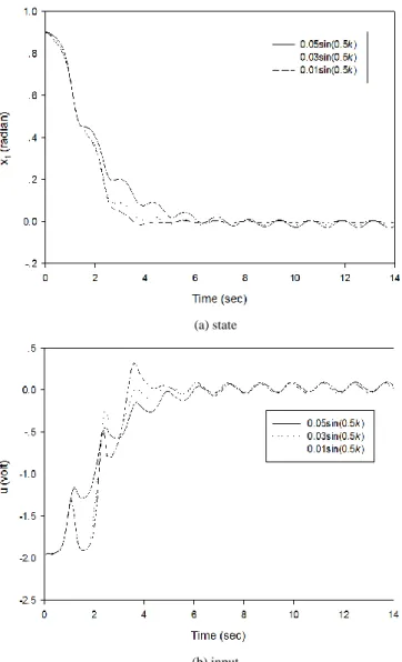
Fig. 1 shows the closed-loop responses of the system when
the uncertain parameter is varied as
) (k
=4.95sin(0.5k)5.05 and the disturbance is varied as )
(k
v = 0.05sin(0.5k) , 0.03sin(0.5k) and 0.01sin(0.5k) , respectively. It can be observed that the state x1(k) is
bounded for all values of uncertain parameter and disturbance
so robust stability is ensured.
(a) state
(b) input
Fig. 1. The closed-loop responses of the system (a) state (b) input. Fig. 2 shows the norm of state feedback gain as a function of time. The norm of state feedback gain increases as time proceeds. This is due to the fact that the input constraint imposes lesser and lesser limit on the state feedback gain. Finally, the input constraint has no effect on the state feedback gain.
Fig. 2. Norm of state feedback gain.
) ] ) ( ) ( [
( 140
0
2 2
k x k uk when the uncertain time-varying parameter and the disturbance are varied as) (k
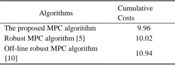
= 4.95sin(0.5k)5.05 and v(k) = 0.05sin(0.5k) , respectively. It is seen that the proposed MPC algorithm can give less cumulative cost than robust MPC algorithm [5] and off-line robust MPC algorithm [10] where the disturbance is not taken into account in the MPC design. Since there will always be some disturbances acting on the real system, they should be explicitly taken into account in the MPC problem formulation as proposed.
TABLEI:THE CUMULATIVE COSTS Algorithms Cumulative
Costs The proposed MPC algoritihm 9.96 Robust MPC algorithm [5] 10.02 Off-line robust MPC algorithm
[10] 10.94
The numerical simulations have been performed in Intel Core 2 Duo (2.53 GHz), 2 GB RAM, using SeDuMi [15] and YALMIP [16] within the Matlab R2008a environment.
V. CONCLUSIONS
In this article, we have presented a synthesis approach of robust MPC using linear matrix inequalities. At each sampling time, a positively invariant set containing the measured state is computed and all future states are restricted to lie within this set without violation of input and output constraints. The proposed algorithm can guarantee both robust stability and constraint satisfaction in the presence of uncertain time-varying parameters and disturbances. In the future work, this idea can be extended to the case where the state cannot be measured. An off-line robust MPC algorithm that solves off-line all of the optimization problems can also be developed. This will reduce on-line computational time while ensuring the same level of control performance.
APPENDICES Appendix A: Proof of Proposition 2.
Lemma 1: [17] Suppose M0 is a symmetric matrix while a and b are vectors with appropriate dimensions. Then, a b2M (1 )a2M (1 1)b2M
for any scalar
0
.
By substituting (4), 1 Q
P into (7) and applying Lemma 1, for any 10, we can see that (7) is satisfied if
. 1 ) ( ) ( ) 1 1 ( ) / ( ] ) ( ) ( [ ) 1
( 21
1 2
1
1
Ak i Bk iKxk i k Q Dk ivk i Q
(21)
Consider the term [A(ki)B(ki)K]x(ki/k)Q21 in (21), let x(ki/k)2Q1 be the maximum value of this term
where 0 1 is a pre-specified scalar
. ) / ( )
/ ( ] ) ( ) (
[ 2 1
2
1
Q
Q x k i k
k i k x K i k B i k
A
(22)Substituting 1
YQ
K , pre-multiplying by T
Q , post-multiplying by Q and applying the Schur complement [18] leads to
0.
) ( )
(
Q Y i k B Q i k A
Q
(23)
From the convexity of the polytopic description, (23) is equivalent to (12).
Consider the term D(ki)v(ki)Q21 in (21), let be the maximum value of this term
D(ki)v(ki)Q21. (24)
Applying the Schur complement leads to
0.
) ( )
(
Q i k v i k D
(25)
From the convexity of the polytopic description, (25) is equivalent to (13).
From (22), (24) and x(ki/k)2Q1 1, (21) is equivalent to
(1 ) (1 1) 1.
1
1
(26)The maximum allowable value of can be calculated by solving
.
) 1 1 (
) 1 ( 1 max
1 1
1
(27)
From (27), we obtain 2 2 1
) 1
(
. Appendix B: Proof of Proposition 3
By defining h as the hth row of the nu-dimensional
identity matrix and applying the Cauchy-Schwarz inequality, we obtain
max ( / )2 ( / )2 2.
0 h h h
i Kxki k Kxki k u (28)
Substituting 1
YQ
K and applying x(ki/k)2Q11
lead to
2.
2 2 1
h
hYQ u
(29)
By applying the Schur complement, we can see that (29) is equivalent to (14).
Appendix C: Proof of Proposition 4
By defining r as the rth row of the ny-dimensional
. ) / 1 ( )
/ 1 (
max 2 2 2
0 r r r
i Cxki k Cxki k y
(30) Substituting (4) and applying Lemma 1, for any 2 0,
lead to
. ) ( ) ( ) 1 1 (
) / ( ] ) ( ) ( [ ) 1 (
2 2
2
2 2
r r
r
y i k v i k CD
k i k x K i k B i k A C
(31)
Consider the term rC[A(ki)B(ki)K]x(ki/k)2 in (31), let Ξr be the maximum value of this term
rC[A(ki)B(ki)K]x(ki/k)2Ξr. (32)
By substituting KYQ1 and applying
1 ) / (
2
2 1
k i k x
Q ,
(32) can be written as
[ ( ) ( ) ] .
2 2 1 1
r rC Aki B kiYQ Q Ξ
(33)
Applying the Schur complement leads to
1,2,...,
. ,, 0 )
) ( ) (
(Ak iQ Bk iY TCT Q Γrr Ξr r ny Γ
(34)
From the convexity of the polytopic description, we can see that (34) is equivalent to (15).
Consider the term rCD(ki)v(ki) 2 in (31), let Φr be the maximum value of this term
rCD(ki)v(ki)2Φr. (35) By applying the Schur complement, we obtain
y
r r
n r
i k v i k D C
Φ
,..., 2 , 1 , 0 1 ) ( )
(
(36)
where Cr is the rth row of C. From the convexity of the polytopic description, (36) can be written as (17). Thus, Φr can be calculated by solving (16) subject to (17).
From (32) and (35), (31) is equivalent to
(1 ) (1 1) 2.
2
2 Ξr Φryr
(37)
The maximum allowable value of Ξr can be calculated by solving
.
) 1 (
) 1 1 ( max
2 2 2
2
r r
r
Φ y
Ξ (38)
From (38), we obtain 2 2
1
)
( r r
r y Φ
Ξ .
REFERENCES
[1] J. H. Lee, “Model predictive control: Review of the three decades of development,” Int. J. Control Autom., vol. 9, pp. 415-424, June 2011.
[2] W. A. Gherwi, H. Budman, and A. Elkamel, “Robust distributed model predictive control: A review and recent developments,” Can. J. Chem. Eng., vol. 89, pp. 1176-1190, May 2011.
[3] S. J. Qin and T. A. Badgwell, “A survey of industrial model predictive control technology,” Control Eng. Pract., vol. 11, pp. 733-764, July 2003.
[4] M. V. Kothare, V. Balakrishnan, and M. Morari, “Robust constrained model predictive control using linear matrix inequalities,” Automatica, vol.32, pp. 1361-1379, October 1996.
[5] W. J. Mao, “Robust stabilization of uncertain time-varying discrete systems and comments on ‘an improved approach for constrained robust model predictive control’,” Automatica, vol. 39, pp. 1109-1112, June 2003.
[6] N. Wada, K. Saito, and M. Saeki, “Model predictive control for linear parameter varying systems using parameter dependent lyapunov function,” IEEE T. Circuits Syst., vol. 53, pp. 1446-1450, December 2006.
[7] P. Bumroongsri and S. Kheawhom, “An ellipsoidal off-line model predictive control strategy for linear parameter varying systems with applications in chemical processes,” Syst. Control Lett., vol. 61, pp. 435-442, March 2012.
[8] Y. I. Lee and B. Kouvaritakis, “Robust receding horizon predictive control for systems with uncertain dynamics and input saturation,”
Automatica, vol. 36, pp. 1497-1504, October 2000.
[9] J. A. Rossiter, B. Kouvaritakis, and M. Bacic, “Interpolation based computationally efficient predictive control,” Int. J. Control, vol. 77, pp. 290-301, February 2004.
[10] P. Bumroongsri and S. Kheawhom, “An off-line robust MPC algorithm for uncertain polytopic discrete-time systems using polyhedral invariant sets,” J. Process Contr., vol. 22, pp. 975-983, July 2012. [11] D. Q. Mayne, M. M. Seron, and S. V. Rakovic, “Robust Model
predictive control of constrained linear systems with bounded disturbances,” J. Process Contr., vol. 41, pp. 219-224, February 2005. [12] D. Q. Mayne, S. V. Rakovic, R. Findeisen, and F. Allgöwer, “Robust output feedback model predictive control of constrained linear systems,” Automatica, vol. 42, pp. 1217-1222, July 2006.
[13] D. Limon, I. Alvarado, T. Alamo, and E. Camacho, “Robust tube-based MPC for tracking of constrained linear systems with additive disturbances,” J. Process Contr., vol. 20, pp. 248-260, March 2010.
[14] J. B. Rawlings and D. Q. Mayne, Model Predictive Control: Theory and Design, 1st ed. Wisconsin, USA: Nob Hill Publishing, 2009, ch. 3, pp. 237-242.
[15] J. F. Sturm, “Using SeDuMi 1.02, a Matlab toolbox for optimization over symmetric cones,” Optim. Method Softw., vol. 11, pp. 625-653, August 1998.
[16] J. Löfberg, “Automatic robust convex programming,” Optim. Method Softw., vol. 27, pp. 115-129, September 2010.
[17] B. C. Ding, Y. Xi, M. T. Cychowski, and T. O. Mahony, “A synthesis approach for output feedback robust constrained model predictive control,” Automatica, vol. 44, pp. 258-264, January 2008.
[18] S. Boyd and L. Vandenberghe, Convex Optimization, 1st ed. Cambridge, U.K.: Cambridge University Press, 2004, ch. 3, pp. 67-108.
Pornchai Bumroongsri was born on 31 January, 1985. He received his bachelor of engineering from Chulalongkorn University in 2008. He obtained his master of engineering and doctor of engineering from Chulalongkorn University in 2009 and 2012, respectively. He is currently a lecturer in the Department of Chemical Engineering, Faculty of Engineering, Mahidol University. His current interests involve robust MPC synthesis, modeling and optimization in chemical processes.