Quantile Based Relevation Transform and its Properties

QUANTILE BASED RELEVATION TRANSFORM AND ITS

PROPERTIES

Dileep Kumar Maladan1

Department of Statistics, Cochin University of Science and Technology, Kerala, India Paduthol Godan Sankaran

Department of Statistics, Cochin University of Science and Technology, Kerala, India Narayanan Unnikrishnan Nair

Department of Statistics, Cochin University of Science and Technology, Kerala, India

1. INTRODUCTION

Relevation transforms, introduced by Krakowski (1973) have attracted considerable in-terest of researchers in survival analysis and reliability theory. Let X andY be two absolutely continuous non-negative random variables, with survival functions ¯F(.)and

¯

G(.)respectively. Consider a component from a population where lifetime has survival function ¯F(x). This component is replaced at the time of its failure at agex, by another component of the same age x from another population. The lifetime of the second component has survival function ¯G(x). LetX#Y denote the total lifetime of the ran-dom variableY given it exceeds a random timeX, (i.eX#Y =d {Y|Y >X}). Then the survival function ofX#Y,

¯

T_X#Y(x) =_F¯_{# ¯G(x) =F}¯_(x)−G¯_(x)Zx 0

1 ¯

G(t)d

¯

F(t), (1)

is called the relevation transform ofX andY. The probability density function (p.d.f.) ofX#Y is obtained as

t_X#Y(x) =T_X0_#Y(x) =g(x) Z x

0 f(t)

¯

G(t)d t. (2)

Grosswaldet al.(1980) provided two characterizations of the exponential distribu-tion based on relevadistribu-tion transform. The concept of dependent relevadistribu-tion transform and

its importance in reliability analysis are given in Johnson and Kotz (1981). Baxter (1982) discussed certain reliability applications of the relevation transform. Shanthikumar and Baxter (1985) provided closure properties of certain ageing concepts in the context of rel-evation transforms. Improved versions of the results in Grosswaldet al.(1980) are given by Lau and Rao (1990). Chukovaet al.(1993) established characterizations of the class of distributions with almost lack of memory property based on the relevation transform.

All these theoretical results and their applications are based on the distribution func-tion. It is well known that any probability distribution can also be specified in terms of its quantile function. For a non-negative random variableX with distribution function

F(x), the quantile functionQ(u)is defined by

Q(u) =F−1(x) =inf{x:F(x)≥u}, 0≤u≤1. (3)

The derivative ofQ(u)is the quantile density function denoted byq(u). Whenf(x) is the probability density function (p.d.f.) ofX, then we get

q(u)f(Q(u)) =1. (4)

One of the basic concepts employed for modelling and analysis of lifetime data is the hazard rate. In quantile set up, Nair and Sankaran (2009) defined hazard quantile func-tion, which is equivalent to the hazard rate,h(x) = f_¯(X)

F(X). The hazard quantile function

H(u)is defined as

H(u) = h(Q(u)) = [(1−u)q(u)]−1. (5)

ThusH(u)can be interpreted as the conditional probability of failure of a unit in the next small interval of time given the survival of the unit until 100(1−u)% point of the distribution. Note thatH(u)uniquely determines the distribution through the identity

Q(u) =

u

Z

0

d p

(1−p)H(p). (6)

Another important concept useful in the context of lifetime studies is the mean resid-ual life. For a non-negative random variableX, the mean residual lifem(x)is defined as

m(x) =E(X−x|X >x) = 1

¯

F(x) Z∞

x ¯

F(t)d t. (7)

Nair and Sankaran (2009) defined the mean residual quantile function, which is the quantile version of the mean residual lifem(x)as

M(u) =m(Q(u)) = 1

1−u Z1

u

M(u)is interpreted as the mean remaining life of a unit beyond the 100(1−u)% of the distribution. M(u)uniquely determinesQ(u)by

Q(u) = Zu

0 M(p)

1−pd p−M(u) +µ, (9)

whereµ=E(X). For a detailed and recent study on quantile functions, its properties, and its usefulness in the identification of models, we refer to Lai and Xie (2006), Nair and Sankaran (2009), Sankaran and Nair (2009), Nair and Vineshkumar (2011), Nair

et al.(2013) and the references therein. Throughout this paper, the terms increasing and decreasing are used in a wide sense, that is, a function g is increasing (decreasing) if g(x)≤ (≥)g(y)for all x ≤y. Whenever we use a derivative, an expectation, or a conditional random variable, we are tacitly assuming that it exists.

The rest of the article is organized as follows. In Section 2, we introduce the quantile version of the relevation transform and study its basic properties. The quantile based relevation transform in the context of proportional hazards model and equilibrium dis-tribution are discussed in Section 3 and Section 4 respectively. Finally, Section 5 sum-maries major conclusions of the study.

2. QUANTILE BASED RELEVATION TRANSFORM

To introduce the quantile based relevation transform between X and Y, we denote

Q_X(u)andQ_Y(u)as the quantile functions corresponding to the distribution functions

F(.)andG(.)respectively. From (1), by taking x = Q_X(u), we define quantile based relevation transform as

T_X#Y(Q_X(u)) =u−G¯(Q_X(u)) Zu

0 1 ¯

G(Q_X(p))d p

=u−(1−Q_Y−1(Q_X(u))) Zu

0

1

(1−Q−1

Y (QX(p)))

d p. (10)

DenoteT∗

X#Y(u) =TX#Y(QX(u))andQ1(u) =QY−1(QX(u)), (10) becomes

T_X∗_#Y(u) =u−(1−Q₁(u)) Zu

0 1

(1−Q₁(p))d p. (11)

IfQ(u)is a quantile function andK(x)is a non-decreasing function ofx, thenK(Q(u))

is again a quantile function (Gilchrist, 2000). Now, since T(.) and Q_Y−1(.)are non-decreasing functions,T_X#Y(Q_X(u))andQ_Y−1(Q_X(p))represent the quantile functions of

F(T−1_(x))andF(G−1_{(x)). We callT}∗

X#Y(u)as the relevation quantile function (RQF). Note that, in general, the quantile based relevation transform is not symmetric, namely

T∗

From (10), we have

T_X∗_#Y(u) =T_X#Y(Q_X(u)) ⇒Q_X#Y(T_X∗_#Y(u)) =Q_X(u)

⇒ Q_X#Y(u) =Q_X(T_X∗−_#1_Y(u)). (12)

Thus, we can compute the quantile function of the relevation random variableX#Y

from the relevation quantile functionT∗

X#Y(u)using the identity (12).

PROPOSITION1. Let X and Y be two random variables with survival functionsF¯(x) andG¯(x)with quantile functions Q_X(u)and Q_Y(u)respectively. Then T∗

X#Y(u)≤u for

all u∈(0, 1).

PROOF. DenoteT_X∗_#Y(u) =u−S(u), where

S(u) = (1−Q₁(u)) Z u

0 1

(1−Q₁(p))d p≥0 for allu∈(0, 1). (13)

SinceQ₁(u) =Q_Y−1(Q_X(u)) =F_Y(Q_X(u)), we haveQ₁(u)∈(0, 1)for allu∈(0, 1). This implies,S(u)≥0 for allu∈(0, 1). From this, we getT∗

X#Y(u)≤ufor allu∈(0, 1). 2 REMARK2. From Proposition 1, we have

T_X∗_#Y(u)≤u for all u∈(0, 1) ⇔T(Q_X(u))≤u for all u∈(0, 1)

⇔Q_X(u)≤Q_X#Y(u) for all u∈(0, 1). (14)

There are many situations in practice where we need to compare the characteristics of two distributions. Stochastic orders are used for the comparison of lifetime distri-butions. We shall consider the following stochastic orders. Their basic properties and interrelations can be seen in Barlow and Proschan (1975) and Shaked and Shanthikumar (2007).

IfX andY are lifetime random variables with absolutely continuous distribution functionsF(x)andG(x)respectively. Let f(x)and g(x)are the corresponding proba-bility density functions. Then we have the following:

(i) X is smaller thanY in the usual stochastic order denoted byX ≤s tYif and only if ¯F(x)≤G¯(x)for allx.

(ii) X is smaller thanY in hazard rate order, denoted byX≤h rY, if and only if ¯ G(x)

¯ F(x)

is increasing inx.

(i) X≤s tY if and only ifQX(u)≤QY(u)for all 0<u<1.

(ii) X ≤h r Y, if and only if HX(u) ≥ HY∗(u), for all 0< u < 1, whereH_X(u) =

h_X(Q_X(u))andH_Y∗(u) =h_Y(Q_X(u)).

Now from (14), sinceQ_X(u)≤ Q_X#Y(u)for all u ∈(0, 1), we get X ≤s t X#Y. Psarrakos and Di Crescenzo (2018) showed thatX ≤h rX#Y. From Nairet al.(2013), we haveX ≤h rY, if and only if

¯

FY(QX(1−u))

u is decreasing inu. This implies 1−T_X#Y(Q_X(1−u)

u =

1−T∗

X#Y(1−u)

u , is decreasing inu.

In the next proposition, we establish the relation between hazard quantile functions of the random variableX#Y andX.

PROPOSITION3. Let H_X#Y(u) and H_X(u)be the hazard quantile functions corre-sponding to the random variables X#Y and X . Then

H_X#Y(T_X∗_#Y(u)) = 1 q_X(u)

d

d u(−log(1−T

∗

X#Y(u))), (15)

or equivalently,

H_X#Y(T∗ X#Y(u))

H_X(u) = (1−u) d

d u(−log(1−T

∗

X#Y(u))). (16)

PROOF. From (12), we have,

Q_X#Y(T_X∗_#Y(u)) =Q_X(u).

Differentiating both sides with respect tou, we get,

q_X#Y(T_X∗_#Y(u))(T_X∗_#Y(u))0=q_X(u).

⇒ 1

q_X#Y(T∗

X#Y(u))(TX∗#Y(u))0

= 1

q_X(u)

⇒ HX#Y(T

∗ X#Y(u))

(T∗ X#Y(u))0

= 1

(1−T∗

X#Y(u))qX(u)

⇒ H_X#Y(T_X∗_#Y(u))q_X(u) = (T

∗ X#Y(u))0

(1−T∗ X#Y(u))

. (17)

From (17), we have,

H_X#Y(T_X∗_#Y(u)) = 1 q_X(u)

d

d u(−log(1−T

∗

X#Y(u))). (18)

Sinceq_X(u) =_(1−u)1_H

PROPOSITION4. Suppose X and Y be two random variables with same support D and Q_{E x p}(u)be the quantile function of the unit exponential distribution. Then

H_X#Y(T_X∗_#Y(u)) = HX(u)

H_Z(u), (19)

where H_Z(u)is the hazard quantile function corresponding to the quantile function Q_Z(u) = Q_{E x p}(T∗

X#Y(u)).

PROOF. SinceXandYhave the same support,D, we have,T∗

X#Y(0) =0 andTX∗#Y(1) = 1. From Gilchrist (2000), we have, ifQ(u)is a quantile function andK(u)is a non-decreasing function of u satisfying the boundary conditionsK(0) =0 and K(1) = 1, thenQ(K(u))is again a quantile function of a random variable with the same support. This gives

Q_Z(u) =Q_{E x p}(T_X∗_#Y(u)) =−log(1−T_X∗_#Y(u)) (20)

is a quantile function with supportQ_Z(0),Q_Z(1) = (0,∞). From (20), we have

H_Z(u) =(1−u) d

d u(−log(1−T

∗ X#Y(u)))

‹−1

(21)

is the hazard quantile function ofQ_Z(u). Now the result (19) follows from (16) and (21),

which completes the proof. 2

EXAMPLE5. Suppose X follows uniform distribution with quantile function Q_X(u) =

θu and Y follows the exponential distribution with quantile function Q_Y(u) =−1_λlog(1− u).Then Q₁(u) =Q_Y−1(Q_X(u)) =1−exp(−λθu),and hence

T_X∗_#Y(u) =u− 1

λθ(1−exp(−λθu)). (22)

The identity(12)is useful for generating random observations of the relevation random variable X#Y . Since T∗

X#Y(u)given in(22)is not directly invertible, we generate the

ran-dom sample of X#Y by first carrying out the numerical inversion of (22)and then using the relation Q_X#Y(u) =Q_X(T∗−1

X#Y(u)).

Relevation quantile function is not unique. There exist different distribution pairs with same relevation quantile function. We illustrate this with the following example.

respectively by

Q_X(u) =−1

λ1

log(1−u);λ₁>0, [exponential distribution(λ₁)],

Q_Y(u) =−_λ1

2

log(1−u);λ₂>0, [exponential distribution(λ₂)],

Q_W(u) = (1−u)−λ11 −1;λ

1>0, [Pareto-II distribution(λ1)], and

Q_Z(u) = (1−u)−λ12 −1;λ₂>0, [Pareto-II distribution(λ₂)].

Now we obtain

Q_Y−1(Q_X(u)) =Q_Z−1(Q_W(u)) =1−(1−u)λλ21.

This gives

T_X∗_#Y(u) =T_W∗_#Z(u) =λ1 (1−u)

λ2/λ1−1+uλ

2 λ2−λ1

.

Note that Q_Y−1(Q_X(u)) is the quantile function of the rescaled beta distribution and T_X∗_#Y(u)is the linear combination of the quantile functions of the rescaled beta and the uniform distributions.

EXAMPLE7. Suppose X follows Govindarajalu distribution with quantile function, Q_X(u) =σ((β+1)uβ−βuβ+1_{)and Y is uniform over the interval(0, 1). In this case,} Q₁(u) =βuβ+1_−(β+1)uβ_+1,then

T_X∗_#Y(u) =

(β(u−1)−1)€_ββ₊u₁ŠβBuβ β+1[

1−β, 0]

β +u. (23)

EXAMPLE8. Let X follows uniform(0,θ₁)and Y follows uniform(0,θ₂), withθ₂≥ θ₁.Then Q₁(u) =€θ1

θ2

Š u and

T_X∗_#Y(u) =u−

1−θ1u

θ2

u−θ1u

2

2θ2

. (24)

SinceT∗

3. PROPORTIONAL HAZARDS RELEVATION TRANSFORM

In reliability theory, proportional hazards model (PHM) plays a vital role in the com-parison of the lifetime of two components. The random variablesX andYsatisfy PHM if

h_Y(x) =θh_X(x), θ >0, (25)

whereh_Y(x)andh_X(x)are the hazard rate functions ofX andY. An equivalent repre-sentation of (25) is

¯

G(x) = (_F¯_(x))θ_{, θ >0. (26)}

For more details on PHM, one could refer to Lawless (2003) and Kalbfleisch and Prentice (2011). WhenYis the PHM ofX with survival functions as in (26), we call the transformation given in (1) as the proportional hazards relevation transform (PHRT).

WhenX is the PHM ofY, denote

T_{P H}∗ (u) =T_X#Y(Q_X(u)) =u−(1−u)θ Z u

0 1

(1−p)θd p

=1−uθ

1−θ −

(1−u)θ

1−θ , u∈(0, 1). (27)

We callT∗

P H(u)as the proportional hazards relevation quantile function (PHRQF).

Whenθ=1,

T_{P H}∗ (u) =T_X#X(Q_X(u)) =u+ (1−u)log(1−u), u∈(0, 1). (28)

PROPOSITION9. Let X and Y be two independent random variables. Then Y is the PHM of X if and only if T∗

P H(u)satisfies the relation

T_{P H}∗ (u) =Q_A(u)−Q_B(u), (29)

where

(i) Q_A(u)and Q_B(u)are the quantile functions of uniform(0,_θ−θ₁)and rescaled beta (0,_θ1₋₁)respectively, whenθ >1,and

(ii) Q_A(u)is rescaled beta(0,₁₋1_θ)and Q_B(u)is uniform(0,₁₋θ_θ), whenθ <1.

PROOF. From (27), we have

T_{P H}∗ (u) = θu

θ−1− 1 θ−1

€

1−(1−u)θŠ. (30)

This can be written as

T_{P H}∗ (u) = ¨θ_u

θ−1− 1

θ−1 1−(1−u)θ

ifθ >1 1

1−θ 1−(1−u)θ

which completes the proof for the ‘if’ part of the proposition. Conversely, assume that

T∗

P H(u)has the form (29), now forθ >1, from (11), we have

T_{P H}∗ (u) =u−ϑ(u) Zu

0 1 ϑ(p)d p=

θu

θ−1− 1 θ−1

€

1−(1−u)θŠ,

whereϑ(u) =1−Q−1

Y (QX(u)). This implies

ϑ(u) Zu

0 1 ϑ(p)d p=

((1−u)θ−(1−u))

1−θ . (32)

Differentiating both sides with respect tou, we get

ϑ0_(u)Zu 0

1 ϑ(p)d p=

θ

1−θ(1−(1−u)θ−

1_{). (33)}

Dividing (33) by (32), we obtain

ϑ0_(u) ϑ(u) =

θ(1−(1−u)θ−1₎

(u−1)(1−(1−u)θ−1)=

−θ

1−u, (34)

which implies

d

d ulog(ϑ(u)) = −θ

1−u. (35)

On integration (35) reduces to

log(ϑ(u)) =log(1−u)θ.

This givesϑ(u)) = (1−u)θ. Now from (11), we have

ϑ(u) =1−Q_Y−1(Q_X(u)) = (1−u)θ,

which gives

Q_X(u) =Q_Y(1−(1−u)θ), or equivalently ¯G(x) = (F¯(x))θ. (36)

Thus,Y is the PHM ofX. Proof for the caseθ <1 is similar and hence the details

are omitted. 2

REMARK10. From Proposition 9, we can see that T_{P H}∗ (u)lies below uniform(0, _θθ₋₁) quantile function whenθ >1and it lies below rescaled beta(0,₁₋1_θ)quantile function when

(a)θ=2.5 (b)θ=0.5

Figure 1 –: (a) Uniform(0,_θ−θ₁)withT_{P H}∗ (u), and (b) rescaled beta(0,₁₋1_θ)withT_{P H}∗ (u).

SinceT∗

P H(u)is a unit support quantile function, we can useTP H∗ (u)with an addi-tional scale parameter for modelling lifetime datasets. Thus, consider the model

Q∗(u) = (

σ1−uθ

1−θ −(1−u) θ

1−θ

ifθ6=1

u+ (1−u)log(1−u) ifθ=1. (37)

The hazard quantile function has the form

H∗(u) =

¨ 1−θ

θσ((1−u)θ_+u−1) ifθ6=1

(σ(u−1)log(1−u))−1 _ifθ=1. (38)

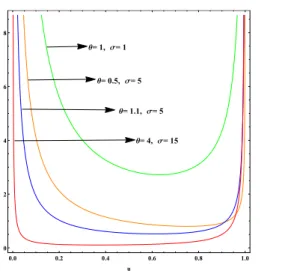
Note that, whenθ=1,q∗_{(u) =} d

d uQ∗(u) =−σlog(1−u), which is the quantile function of an exponential distribution with meanσ. Thusq∗_{(u)is non decreasing when} θ=1.H∗_{(u)is bathtub shaped for all choices of the parameters. Change point ofH}∗_(u) isu₀=1−€1_θŠ

1 θ−1

q= 0.5, s= 5

q= 4, s= 15

q= 1.1, s= 5

q= 1, s= 1

0.0 0.2 0.4 0.6 0.8 1.0 0

2 4 6 8

u

H

H

u

L

Figure 2 –: Hazard quantile function for different choices of parameters.

L-moments. The first and secondL-moments are given by

L₁= Z1

0

Q(u)d u=θ € ₁

θ+1− 1 2

Š

σ

1−θ , (39)

and

L₂= Z1

0

(2u−1)Q(u)d u= θ

€ ₁

θ2_+3θ+2−

1 6

Š

σ

1−θ . (40)

We equate sampleL−moments to corresponding populationL-moments. Letx₁,x₂, ...,x_n

be a random sample of size n from the population with quantile function (37). To define the L- moments of a sample, we first take the order statistics of the sample:

x₍₁₎≤x₍₂₎≤...≤x_(n)and define the sampleL-moments,l_l,l₂, ...,l_nby

l_r=Xr−1

k=0

p_r,k b_k, (41)

where

b_k= ₁

n ‹ n

X

i=1

(i−1)(i−2)...(i−k)

In particular, the first two sampleL−moments are given by

l₁ = ₁

n ‹ n

X

i=1 x_(i),

l₂= ₁

2

‹ _n

2

−1 n

X

i=1

i−1

1

−

n−i

1

x_(i),

(43)

wherex_(i)is thei-th order statistic. For estimating the parametersθandσ, we equate the above two sampleL−moments to corresponding populationL-moments given in (39) and (40). The parameters are obtained by solving the equations

l_r=L_r; r=1, 2. (44)

The estimates of the parameters are obtained as, ˆθ=2.004, ˆσ=43.988. Midhuet al.

(2013) fitted the data using the class of distributions with linear mean residual quantile function. The quantile function of the model proposed by Midhuet al.(2013) is

Q(u) =−(c+µ)log(1−u)−2c u,µ >0,−µ <c< µ. (45)

Mudholkar and Srivastava (1993) analyzed this data using an exponentiated-Weibull model with distribution function

F(x) = (1−exp(−(λx)γ)), λ >0,γ >0. (46)

To compare the performance of the aforementioned models with the proposed quan-tile function, we use the Akaike information criterion (AIC)(Akaike, 1974). The AIC is defined by

AI C=2k−2 log(Lˆ),

where ˆLis the estimate of likelihood function. The AIC measure for the proposed model is 151.5, whereas the AIC’s for the models proposed by Midhuet al.(2013) and Mud-holkar and Srivastava (1993) are 153.45 and 748.41 respectively. On the basis of AIC values, our model gives better fit.

4. RELEVATION TRANSFORM WITH EQUILIBRIUM DISTRIBUTION

The equilibrium distribution is a widely accepted tool in the context of analysis of ageing phenomena. The equilibrium distribution associated with the random variable X is defined by the survival function

¯

F_E(x) = 1

µ_X

Z∞

x ¯

Settingx=Q_X(u), from Nairet al.(2013), we have

F_E(Q_X(u)) = 1

µX

Zu

0

(1−p)q_X(p)d p, (48)

where the integral

φX(u) = 1 µX

Zu

0

(1−p)q_X(p)d p (49)

is called the scaled total time on test transform (TTT) of the random variableX. For various properties and applications ofφ_X(u), one could refer to Nairet al.(2013).

From (48) and (49), we have

Q_X(u) =Q_E(φ_X(u)), (50)

whereQ_E(.)is the quantile function corresponding to the equilibrium distribution of

X.

PROPOSITION11. Let X and Y be two non-negative random variables. Then Y is the equilibrium random variable of X if and only if

T_X∗_#Y(u) =u−(1−φX(u))

Zu

0

d p (1−φX(p))

. (51)

PROOF. AssumeY is the equilibrium random variable ofX. From (10), we have

T(Q_X(u)) =u−(1−Q_Y−1(Q_X(u))) Z u

0

1

(1−Q−1

Y (QX(p)))

d p. (52)

SinceYis the equilibrium random variable ofX, we have

Q_X(u) =Q_Y(φ_X(u)). (53)

Now using (53) in (52), we get

T_X∗_#Y(u) =u− 1−Q_Y−1(Q_Y(φX(u)))

Zu

0

1

1−Q_Y−1(Q_Y(φ_X(p)))d p,

=u−(1−φX(u))

Z u

0

d p (1−φX(p))

. (54)

Conversely, assume (51) is true. Now from (11), we have

u−(1−Q₁(u)) Zu

0 1

(1−Q₁(p))d p=u−(1−φX(u)) Zu

0

d p (1−φX(p))

Taking derivative on both sides with respectu, and simplifying, we get

Q₁(u) =φX(u)

⇔ Q_Y−1(Q_X(u)) =φ_X(u) ⇔ Q_X(u) =Q_Y(φ_X(u)).

ThusYis the equilibrium random variable ofX, which completes the proof. 2

COROLLARY12. Suppose Y is the equilibrium random variable of X . Then T∗ X#Y(u)

uniquely determinesφ_X(u)through the identity

φX(u) =1−exp

Zu

0

(T∗ X#Y(p))0

T∗

X#Y(p)−p

d p

. (55)

PROOF. From (51), we have

(1−φX(u))

Zu

0

d p (1−φX(p))

=u−T_X∗_#Y(u). (56)

Differentiating both sides with respect tou, we get

1−φ0 X(u)

Zu

0

d p (1−φX(p))

=1−(T_X∗_#Y(u))0

⇔ φ0X(u)

Zu

0

d p (1−φX(p))

= (T_X∗_#Y(u))0. (57)

From (56), we haveRu

0 d p

(1−φX(p))= u−T

∗ X#Y(u)

(1−φX(u)). Inserting this in (57), we obtain

φ0 X(u) 1−φX(u)

= (TX∗#Y(u))0

u−T∗ X#Y(u)

,

or d

d u(log(1−φX(u))) = (T∗

X#Y(u))0

T∗

X#Y(u)−u ,

which gives

φ_X(u) =1−exp

Zu

0

(T∗ X#Y(p))0

T∗

X#Y(p)−p

d p

.

This completes the proof. 2

REMARK13. From Nairet al.(2013), we haveφ_X(u)uniquely determines the distri-bution through the relation

Q(u) = Z u

0

µXφ0X(p)

1−p d p. (58)

Now, from Corollary 12, we have T∗

X#Y(u)uniquely determines the baseline

EXAMPLE14. Let X be distributed as generalized Pareto with quantile function

Q_X(u) = b a

”

(1−u)−a+a1−1

—

, b>0,a>−1. (59)

SinceµX =b,we get

φX(u) = 1 µ

Zu

0

(1−p)q_X(p)d p=”1−(1−u)a+11—. (60)

Hence, the equilibrium random variable Y has its quantile function as, Q_Y(u) =Q_X(φ−1 X (u)).

Thus from(59)and(60), we obtain

Q_Y(u) = b a

(1−u)−a₋₁

. (61)

Using(51), we get

T_X∗_#Y(u) = 1 a €

(a+1)€1−(1−u)a+11Š−uŠ. (62)

From Nairet al.(2013),φ_X(u)andM_X(u)are related through the identity

M_X(u) =1−φX(u)

1−u . (63)

Inserting (63) in (51), we get

T_X∗_#Y(u) =u−(1−u)M_X(u) Zu

0

d p

(1−p)M_X(p). (64)

ThusM_X(u)uniquely determinesT∗

X#Y(u), whenYcorresponds to the equilibrium distribution ofX.

EXAMPLE15. Suppose X follows linear mean residual quantile function distribution with M_X(u) =µ+c u,and Q_X(u)as in(45)(Midhuet al., 2013). In this case

T_X∗_#Y(u) =u+(1−u)(c u+µ)log €_µ−µu

c u+µ

Š

c+µ . (65)

In the next proposition, we provide a characterization for the exponential distribu-tion usingT_X∗_#Y(u), whenY is the equilibrium random variable ofX.

PROPOSITION16. Let X be a non-negative random variable and Y be the correspond-ing equilibrium random variable. Then X has exponential distribution if and only if

PROOF. AssumeXfollows exponential distribution with quantile functionQ_X(u) = −1

λ log(1−u),λ >0. We getµX = 1

λ andφX(u) =u. SinceφX(u) =u, from (50), we haveQ_X(u) =Q_Y(u). This implies

T_X∗_#Y(u) =T_X∗_#X(u).

Conversely, we have,T∗

X#Y(u) =TX∗#X(u)for allu∈(0, 1). Now from (11), we have

T_X∗_#Y(u) =u+ (1−u)log(1−u). (67)

Now using (55), we getφ_X(u) =u. Thus from (58), the baseline quantile function ofX is obtained asQ_X(u) =−µXlog(1−u), which is exponential. This completes the

proof. 2

In ¯T_X#Y(x), given in (1), if we take ¯F(x) =_µX1 R∞

x G¯(t)d tandu=G(x), we get

1−T_X#Y(Q_Y(u)) = Ru

0(1−p)qY(p)d p

µ_Y + (1−u)

Zu

0 1 µ_Yd p,

=1− Ru

0(1−p)qY(p)d p µY

+(1−u)u

µY ,

which implies

T_X#Y(Q_Y(u)) =1−φY(u) +

(1−u)u

µY ,

=1−(1−u)

µY

[M_Y(u) +u], (68)

whereM_Y(u)is the mean residual quantile function ofY.

5. CONCLUSION

The present work introduced an alternative approach to relevation transform using quantile functions. Various properties and applications of quantile based relevation transform were discussed. Quantile based relevation transform in the context of propor-tional hazards and equilibrium models were presented. The PHRQF model is applied to a real lifetime data set. It was proved thatT∗

X#Y(u)uniquely determines the distribution ofX, whenY is the equilibrium random variable ofX. We can develop quantile based analysis of a sequence of random variables constructed based on the relevation trans-form. The identity (66) can be used to test exponentiality. For this, one has to develop non-parametric estimator ofT∗

ACKNOWLEDGEMENTS

We thank the referee and the editor for their constructive comments. The first author is thankful to Kerala State Council for Science Technology and Environment (KSCSTE) for the financial support.

—————————————————————-REFERENCES

H. AKAIKE(1974).A new look at the statistical model identification. IEEE Transactions on Automatic Control, 19, no. 6, pp. 716–723.

R. E. BARLOW, F. PROSCHAN(1975). Statistical Theory of Reliability and Life Testing: Probability Models. Holt, Rinehart and Winston, New York.

L. A. BAXTER(1982).Reliability applications of the relevation transform. Naval Research Logistics, 29, no. 2, pp. 323–330.

S. CHUKOVA, B. DIMITROV, Z. KHALIL(1993). A characterization of probability dis-tributions similar to the exponential. Canadian Journal of Statistics, 21, no. 3, pp. 269–276.

W. GILCHRIST(2000).Statistical Modelling with Quantile Functions. CRC Press, Abing-don.

E. GROSSWALD, S. KOTZ, N. L. JOHNSON(1980).Characterizations of the exponential distribution by relevation-type equations. Journal of Applied Probability, 17, no. 3, pp. 874–877.

J. R. M. HOSKING(1990). L-moments: analysis and estimation of distributions using linear combinations of order statistics. Journal of the Royal Statistical Society. Series B, pp. 105–124.

J. R. M. HOSKING, J. R. WALLIS(1997).Regional frequency analysis: An approach based on L-moments. Cambridge University Press, Cambridge.

N. L. JOHNSON, S. KOTZ(1981). Dependent relevations: Time-to-failure under depen-dence. American Journal of Mathematical and Management Sciences, 1, no. 2, pp. 155–165.

J. D. KALBFLEISCH, R. L. PRENTICE(2011). The Statistical Analysis of Failure Time Data, vol. 360. John Wiley & Sons, New York.

C. D. LAI, M. XIE (2006). Stochastic Ageing and Dependence for Reliability. Springer Verlag, New York.

K. S. LAU, B. P. RAO(1990). Characterization of the exponential distribution by the rele-vation transform. Journal of Applied Probability, 27, no. 3, pp. 726–729.

J. F. LAWLESS(2003). Statistical Models and Methods for Lifetime Data. John Wiley & Sons, New York.

N. N. MIDHU, P. G. SANKARAN, N. U. NAIR(2013). A class of distributions with the linear mean residual quantile function and it’s generalizations. Statistical Methodology, 15, pp. 1–24.

G. S. MUDHOLKAR, D. K. SRIVASTAVA(1993).Exponentiated Weibull family for analyz-ing bathtub failure-rate data. IEEE Transactions on Reliability, 42, no. 2, pp. 299–302.

N. U. NAIR, P. G. SANKARAN(2009).Quantile-based reliability analysis. Communica-tions in Statistics-Theory and Methods, 38, no. 2, pp. 222–232.

N. U. NAIR, P. G. SANKARAN, N. BALAKRISHNAN(2013).Quantile-Based Reliability Analysis. Springer, Birkhauser, New York.

N. U. NAIR, B. VINESHKUMAR(2011). Ageing concepts: An approach based on quantile function. Statistics & Probability Letters, 81, no. 12, pp. 2016–2025.

G. PSARRAKOS, A. DICRESCENZO(2018).A residual inaccuracy measure based on the relevation transform. Metrika, 81, pp. 37–59.

P. G. SANKARAN, N. U. NAIR(2009). Nonparametric estimation of hazard quantile function. Journal of Nonparametric Statistics, 21, no. 6, pp. 757–767.

M. SHAKED, J. G. SHANTHIKUMAR(2007). Stochastic Orders. Springer Verlag, New York.

J. SHANTHIKUMAR, L. A. BAXTER(1985).Closure properties of the relevation transform. Naval Research Logistics, 32, no. 1, pp. 185–189.

W. J. ZIMMER, J. B. KEATS, F. WANG(1998). The Burr XII distribution in reliability analysis. Journal of Quality Technology, 30, no. 4, p. 386.

SUMMARY