Estimation sensorless vector control of induction drive performance with dynamic resistance tuning

(1)

Estimation sensorless vector control of induction drive performance

with dynamic resistance tuning

Bharti Yadav1 Md. Ashfaque Khan2

M.Tech Scholar NIIST Bhopal Asso. Prof. of Dept. Ex. NIIST Bhopal

1MMMMK11222

Abstract- This paper presents the outcomes

of a sensor less indirect stator-flux-oriented control (ISFOC) implementation to an induction motor drive with stator resistance tuning. The estimation of speed and stator resistance is based only on measurement of stator currents. The error of the measured q-axis current from its reference value feeds the proportional plus integral (PI) controller, the output of which provides the estimated slip frequency. Feed forward compensator operates on a Synchronous frame and Owing to its advantages; an IP controller is used for rotor speed regulation.

This work focuses on speed estimation techniques for sensor less closed-loop speed Control of an induction machine based on indirect field-oriented control technique. Details of theories behind the algorithms are stated and their performances are verified by the help of simulation.

Keywords: Speed estimation, sensor less closed-loop indirect field oriented control (ISFOC), flux estimation, Resistance tuning, Induction motor.

NOMENCLATURE

vds, vqs d, q-axis stator voltage components.

ids, iqs d, q-axis stator current components.

Φds, Φqs d, q-axis stator flux components.

Rs, Rr Stator and rotor winding resistance.

Ls, Lr Stator and rotor self-inductance.

M Mutual inductance. Np Number of pole pairs.

p Δ=d/dt Differential operator.

ωs, ωr Synchronous and rotor angular speed.

ωsl Slip angular speed (ωs − ωr).

Te, Tl Electromagnetic and load torque.

J Moment of inertia. f Friction constant.

τs, τr Stator and rotor time constant.

Kp Proportional gain of the integral plus

proportional(IP) speed controller. Ki Integral gain of the IP speed controller.

Kip Proportional gain of the proportional

plus integral (PI) current controller. Kii Integral gain of the PI current controller.

Kωp Proportional gain of the PI slip speed

estimation controller.

Kωi Integral gain of the PI slip speed

estimation controller.

kri Integral gain of the estimated stator

resistance variation controller. σ Total leakage constant.

∧, * Estimated and reference value.

I. Introduction

V

ECTOR control has been widely used for the high performance drive of the induction motor. The Technique can be classified into two categories namely direct and indirect flux vector orientation control schemes. In the existing literatures, [1 to 10] many approaches have been suggested for speed sensor less vector control induction motor drives. These methods are based on the following schemes: Harmonic caused by machine saliency ,Model Reference Adaptive System (MRAS),Extended Kalman filter (EKF),Artificial Neural Network (ANN), Extended Luenberger Observers, Instantaneous Reactive Power

For indirect control methods, some kind of parameter adaptation is required in order to obtain high performance sensor less vector control drive. At very low speed, Indirect Stator Flux Oriented Control (ISFOC) of induction motor drive is particularly sensitive to an accurate stator resistance value in the stator flux. To overcome this problem, online tuning stator resistance variation of the induction motor is essential in order to maintain the dynamic performance of a sensor less ISFOC drive

The current work utilizes a novel method of sensor less ISFOC induction motor drive with stator resistance tuning and dynamic feed forward decoupling scheme able to operate down to zero speed, which require only current and dc bus voltage sensors. Online estimation of stator resistance variation is obtained by means of the error between d-axis stator current and that generated by the algorithm command. By using a pure integral controller, we can estimate stator resistance variation.

II. Induction Motor-Flux-Orientation model

The ISFOC scheme, some simplifying assumptions are made in order to reduce the complexity of the drive model and as the stator flux vector which acts along the direct axis, if kept constant,i.e. Φds = Φs and Φqs

= 0. The dynamic model of an induction motor can be represented, according to the usual d-axis and q-axis components in a synchronous rotating frame as

(2)

(1)

vds = Rs (τ_τs _r+τr ) 1 +

 τs τr

τs + τ rp ids

−σLs ωsl iqs −

s

τr

vqs = Rs (τ_τs +τr )

r 1 +

 τs τr

τs + τ rp iqs

+σLs ωsl ids + ωrs (2)

_s= Ls

1 + τr p

1 + τr p ids −

σ τr Ls ωsl

1 + τr p iqs

(3)

(4)

ωsl =

Ls

τr

1 + τr p

_s− σ ids Ls iqs

Te = Np _siqs

(5)

From the above relations it can be inferred that, if the stator flux is kept constant, the torque can be controlled by controlling the q-axis current.

 = 1 − M2 Ls Lr , τs = Ls Rs ,and

τr = Lr Rr

The electromagnetic torque equation and the electrical angular speed motor are related by

Jdωr

dt + fωr = Np Te − Tl

(6)

III. Feed-forward Decoupling Controller

It can be seen that the d-axis and q-axis voltage equations are coupled by the terms−σLs ωsl iqs −_τs

r - and

σLs ωsl ids + ωrs . These terms are considered as

disturbances and are cancelled by using a decoupling method that utilizes nonlinear feedback of the coupling voltages. If the decoupling method is implemented the voltage equations become

vd = vds + Ed =

Rs (τ_s+τ_r)

τr 1 +

 τs τr

τs + τ rp ids

(7)

vq = vqs + Eq =

Rs (τ_s+τ_r)

τr 1 +

 τs τr

τs + τ rp iqs

(8)

Where

Ed = σLs ωsl iqs −_τs

r and Eq = −σLs ωsl ids −

ωrs ; Ed and Eq

Respectively is the d- and q-back electromotive force (EMF). Thus, the dynamics of the d-axis and q-axis currents can be represented by simple linear first-order differential equations. And it becomes possible to effectively control the currents with PI controller.

For the decoupling controller shown in figure 1, it should be noted that the estimated Values, denoted by , are introduced to cancel out the coupling terms in the induction motor model. If we assume that the back EMFs are canceled by the feed forward compensation term, we obtain

Gd p = Gq p =

Kc

1 + τr p

(9)

WhereKc = τ_r Rs ( τr + τr ) is a gain and

𝝉𝒄 =_𝝉 𝝉𝒔 𝝉𝒓

𝒔 + 𝝉𝒓 is a time constant. The closed-loop current

transfer function is

ids p

iqs p =

ωni2 1 +

Kip

Kii p

p2_{+ 2}__ω

nip + ωni2

(10)

Where,𝜔𝑛𝑖 = 𝐾𝑐_𝜏𝐾𝑖𝑖

𝑐 𝑎𝑛𝑑  =

1+𝐾𝑐+𝐾𝑖𝑝

2𝜔_𝑛𝑖𝜏_𝑐

,

ωni and ξ denote natural frequency and damping ratio,

respectively.

When the dynamics of the d- and q-axes currents are equivalent, the PI gains can be copied to the q-axis controller as well.

(3)

Figure.2 SIMULINK block diagram of the conventional PI controller with feed forward decoupling method.

IV. Sensorless Speed Control Algorithm

The sensorless speed control algorithm is implemented with the help of slip speed and stator resistance variation estimators, which are explained in following sections.

A. Slip speed estimation

The slip speed can be estimated by using the regulation in closed-loop q-axis current given by Eq 3 & Eq 4, by neglecting the term (𝜎𝜏𝑟𝜔𝑠𝑙)2 the following

relation between slip speed 𝜔𝑠𝑙 and q-axis stator current

iqs is obtained

𝜔𝑠𝑙 ≈

𝐿𝑠(1 +𝜏𝑟𝑝)2

(1 − 𝜎)𝜏𝑟Φ𝑠 𝑖𝑞𝑠

(11)

The slip speed as shown above is a second order differential equation for qudrature axis current. And we can obtain stator flux reference and slip angular frequency estimator from reference currents by,

𝑝𝑖𝑑𝑠∗ = −

1

𝜏𝑟 𝑖𝑑𝑠

∗ ₊1 +𝜏𝑟𝑝

 𝐿𝑠𝜏𝑟 𝜙𝑠

∗₊

_𝜔

𝑠𝑙𝑖𝑞𝑠∗

(12)

𝑝𝑖𝑞𝑠∗ = −_1_𝜏 𝑟 𝑖𝑞𝑠

∗ ₊ 𝜙𝑠

∗

 𝐿𝑠

𝜔

𝑠𝑙−

𝜔

𝑠𝑙𝑖𝑑𝑠 ∗

(13)

Two error components exists between reference and measurement in the d-axis and q-axis currents,

𝜀

𝑑 = 𝑖𝑑𝑠∗ − 𝑖𝑑𝑠 &

𝜀

𝑞= 𝑖𝑞𝑠∗ − 𝑖𝑞𝑠 and the slip speed

error is defined by;

𝜀

_𝜔𝑠𝑙

= 𝜔

_𝑠𝑙

− 𝜔

_𝑠𝑙 (14)

We express the measured and reference variables according to these errors, we obtain

p

𝜀

_𝜀

d q =

− 1 στr ωsl

−ωsl −_στ1

r

𝜀

_𝜀

d q +

−i_qs ids− ϕs

∗

σLs

𝜀

ωsl (15)

Graphical study of the variation of stator current error according to slip speed error indicated that the q-axis current error varies almost linearly with the variation of the slip speed error and that the d-axis current error is weak and negligible in relation to𝜀𝑞. Thus, it is possible to

use only the q-axis error 𝜀𝑞 for the estimation of slip speed

as,

(1 + 𝜎𝜏𝑟𝑝)

𝜀

𝑞=𝜎𝜏𝑟(𝑖𝑑𝑠−

𝜙_𝑠∗ 𝜎𝐿𝑠)

𝜀

𝜔𝑠𝑙

(16)

The block diagram of slip speed estimation. Implemented in SIMULINK, as shown in figure 3

Figure.3 SIMULINK block diagram of slip speed estimation.

The d-axis stator current is assumed equal to the steady state current ids0.we establish the transfer function

connecting the slip speed error to the q-axis current,

εq(p)

ε_{𝜔 𝑠𝑙}(p)=

𝑟(𝑖𝑑𝑠−_𝜙 𝑠∗_𝐿𝑠)

𝑟𝑝+1

(17)

A PI controller is used for slip speed estimation with the sign of the gain K0 being negative, to obtain

positive gains of the regulator, the inversion of sign will be carried out on the comparative of the q-axis current. It should be noted that the dynamic slip speed error is now represented by the simple linear first-order differential equation with q-axis current error and it becomes possible to effectively control slip speed error with a PI controller. Thus, the estimated slip speed is given by the closed-loop transfer function can be expressed as

(4)

𝜔

_𝑠𝑙 = 𝐾𝜔𝑝 𝑝+𝐾𝜔𝑖

𝑝 (𝑖𝑞𝑠− 𝑖𝑞𝑠 ∗ ₎

(18)

𝜔𝑛 =

𝐾0𝐾𝜔𝑖

𝜎𝜏𝑟 𝑎𝑛𝑑  =

𝐾0𝐾𝜔𝑝+ 1

2𝜔𝑛 𝜎𝜏𝑟

(19)

ωn and ξ denote natural frequency and damping ratio,

respectively.

By setting the damping ratio ξ = 1, the characteristic equation of the closed-loop system admits a double pole. For a given damping ratio, the second-order systems give a constant value for ωntr = k. For a damping

ratio ξ = 1, we obtain ωntr ≈ 4.75. The proportional and

integral gains of the PI controller are given as

𝐾𝜔𝑝 =

2𝜎𝜏_𝑟_𝑡𝑟𝑘 −1

𝐾0 (20)

𝐾𝜔𝑖 =

𝜎𝜏𝑟 _𝑡𝑘 𝑟

2

𝐾0

(21)

Where tr is the response time.

B. Stator Resistance Variation estimation

So as to choose correctly the variable that allows us to identify stator resistance variation, we graphically studied the variation of the d-axis and q-axis current error according to the stator resistance variation that the d-axis current error strongly varies almost linearly with stator resistance variation ΔRs. The q-axis current error remains

weak and can be neglected in relation to the d-axis current error. Thus, we use only d-axis current error for the estimation of stator resistance variation. The d-axis reference stator voltage is given by

𝑣𝑑𝑠∗ = 𝑅𝑠0+ Δ𝑅s 𝑖𝑑𝑠+ 𝑑_𝑑𝑡𝑑𝑠 − 𝜔𝑞𝑞𝑠 (22)

Establishing the equality between the two expressions, we obtain

𝜀𝑑=_𝑅𝑖𝑑𝑠

𝑠0+ Δ𝑅s−

1 𝑅_𝑠0

𝑑𝜀𝑞𝑠

𝑑𝑡 −

1

𝑅_𝑠0𝜔𝑠𝜀𝑞𝑠

(23)

The block diagram of estimation of stator resistance variation implemented in SIMULINK, as shown in figure 4

Figure 4 SIMULINK block diagram of stator resistance variation

For steady state equation (24)can be put in the form,

(24)

𝜀𝑑 = 𝜀𝑑1− 𝜀𝑑2

Where,

𝜀𝑑1=_𝑅𝑖𝑑𝑠

𝑠0Δ𝑅s

&

𝜀𝑑2=

1

𝑅𝑠0𝜔𝑠𝜀𝑞𝑠

The simulation results studied in show that the two terms εd1 and εd2 vary linearly with stator resistance

variation ΔRs. So a first approximation can be used as

𝜀𝑑2= 𝑘1Δ𝑅𝑠

(25)

For a small stator resistance variation, the d-axis current can be regarded as constant. Thus, we can establish the transfer function connecting the stator resistance variation ΔRs to the d-axis current error by

𝜀_𝑑(𝑝) ∆𝑅𝑠(𝑝)=

𝑖_𝑑𝑠

𝑅𝑠0− 𝑘1

Where,

𝑘1 ≤_𝑅𝑖𝑑𝑠

𝑠0 (26)

In steady state, to cancel stator resistance variation error estimation, we chose an integral regulator type so that

𝑅 s=𝑘_𝑝𝑟𝑖(𝑖𝑑𝑠− 𝑖𝑑𝑠∗ ) (27)

Where kri is the integral controller gain of the

stator resistance variation estimation.

(5)

variation ΔRs. Fig. 6 shows the block diagram of the

simulated sensorless SFOC of induction motor drive system with stator resistance tuning.

V. Simulation Results

The model topologies of ISFOC as discussed in previous sections have been developed in Matlab © Simulink ® and the results obtained are validated with the help of published literature.

Figure 5 Block diagram of sensorless stator-flux-oriented induction motor drive system.

Figure 6 SIMULINK block diagram of sensorless

stator-flux-oriented induction motor drive system.

The basic block diagram of an SFOC topology is given in figure 5.As shown the voltage-source inverter (VSI) utilizes a diode rectifier front-end with dc bus voltage. And for the minimization of sensors used, only two stator currents and dc bus voltage are measured, the estimated and realspeed of the induction motor and Load torque is compared with the actual speed for validating the accuracy of estimation.

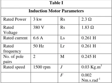
The induction motor parameters values are given in Tables I The estimated d, q components of stator flux are obtained from the stator voltage model of induction motor in d, q reference frame.

Table I

Induction Motor Parameters

Rated Power 3 kw Rs 2.3 Ω

Rated Voltage

380 V Rs 1.83 Ω

Rated current 6.6 A Ls 0.261 H

Rated frequency

50 Hz Lr 0.261 H

No. of pole pairs

2 M 0.245 H

Rated speed 1500 rpm J 0.03 Kg.m3 F 0.002

Nm.s.rad-1

The motor parameters estimated in by ISFOC are highly inaccurate; this difference is due to the fact that the ISFOC method operates in open loop, without any feedback from the stator flux error. In order to avoid such a situation, it is necessary to provide the ISFOC drive system with accurate stator resistance value, effect of temperature rises, windage, etc.

It should be noted that we have considered the rotor resistance to be constant. However, like stator resistance, rotor resistance also depends on temperature, which has an influence on the decoupling between the flux and torque and optimal controller.

In addition to the machine parameters the various gains for the PI controllers used for slip speed and flux estimation schematics; these are given in table II below:

Table II Controller Gains

Kp 0.5 Kwp 35.35 Ki 6 Kip 6.5 Kwi 9780 Kii 673.5

(6)

I.

Speed response

(a)

Experimental results of speed response.

II. Motor phase current

(c)

Experimental results of

Motor phase current.

III.Load torque & Quadrature axis current

(e)

Experimental results of Load torque &

Quadrature axis current.

(b)

Simulation results of speed response.

(d)

Simulation results of

Motor phase current.

(f)

Simulation results of Load torque.

(7)

IV. Simulation results for 3-phase voltages.

(g)

V.

Simulation results for dc bus voltage.

(h)

VI.

Simulation results for load torque.

(i)

VI

. C

onclusion

This paper makes a contribution to the issue of sensor less SFOC of induction motor drive with stator resistance tuning and dynamic feed forward decoupling scheme. A new method has been presented that is able to perform at nominal, low, and zero sensor less speed control of induction motor drive. What is really new, compared to previous works in the literature, is the sensorless control method using slip angular speed estimation with stator resistance tuning based on the error between d, q axis stator currents and that generated by the algorithm command, respectively. Simulation results have shown the practical feasibility of the proposed approach that allows one to estimate both rotor speed and stator resistance variationfor a wide speed range. All simulation results confirm the good dynamic performances of the

developed drive systems and show the validity of the proposed method.

References

[1] Md.Boussak,,Kamel Jarry “High performance sensorless indirect stator flux orientation control of induction motor drive,”

IEEE Trans. Ind. Electron., vol. 53, no. 1, pp. 100–110, Feb. 2006.

[2] F. J. Lin, R. J. Wai, C. H. Lin, and D. C. Liu, “Decoupling stator-flux oriented induction motor drive with fuzzy neural network uncertainly observer,” IEEE Trans. Ind. Electron., vol. 47, no. 2, pp. 356–367, Apr. 2000.

[3] S. Suwankawin and S. Sangwongwanich, “A speed sensorless

IM drive with decoupling control and stability analysis of speed estimation,” IEEE Trans. Ind. Electron., vol. 49, no. 2, pp. 444– 455, Apr. 2002.

[4] D. Drevensek, D. Zarko, and T. A. Lipo, “A study of

sensorless control of induction motor at zero speed utilizing high frequency voltage injection,” EPE J., vol. 12, no. 3, pp. 7–11, Aug. 2003.

[5] A. Consoli, G. Scarcella, and A. Testa, “Using the induction

motor as flux sensors: New control perspectives for zero-speed operation of standards drives,” IEEE Trans. Ind. Electron., vol. 50, no. 5, pp. 1052–1061, Oct. 2003.

[6] C. Schauder, “Adaptive speed identification for vector control of induction motors without rotational transducers,” IEEE Trans. Ind. Appl., vol. 28, no. 5, pp. 1054–1061, Sep./Oct. 1992. [7] L. Zhen and L. Xu, “Sensorless field orientation control of induction machines based on mutual MRAS scheme,” IEEE Trans. Ind. Electron., vol. 45, no. 5, pp. 824–831, Oct. 1998. [8] Y. R. Kim, S. K. Sul, and M. H. Park, “Speed sensorless

vector control of induction motor using an extended Kalman filter,” IEEE Trans. Ind. Appl., vol. 30, no. 5, pp. 1225–1233, Sep./Oct. 1994.

[9] K. L. Shi, Y. K. Wong, and S. L. Ho, “Speed estimation of an

induction motor drive using an optimized extended Kalman filter,” IEEE Trans. Ind.Electron., vol. 49, no. 1, pp. 124–133, Feb. 2002.

[10] S. H. Kim, T. S. Park, and G. T. Park, “Speed sensorless