STATISTICAL METHODS FOR MASS SPECTROMETRY
PROTEOMICS EXPERIMENTS
Jonathon O’Brien
A dissertation submitted to the faculty at the University of North Carolina at Chapel Hill in partial fulfillment of the requirements for the degree of Doctor of Philosophy in
the Department of Biostatistics.
Chapel Hill 2016
Approved by: Bahjat Qaqish
Joseph Ibrahim
Wei Sun
Mengjie Chen
c
2016
ABSTRACT
Jonathon O’Brien: Statistical Methods for Mass Spectrometry Proteomics Experiments (Under the direction of Bahjat Qaqish)
DNA makes RNA makes proteins is the central dogma of molecular biology. While the
measurement of RNA has dominated the landscape of scientific inquiry for many years, often the
true outcome of interest is the final protein product. Microarray and RNAseq studies do not tell
researchers anything about what happens during and after translation. For this reason interest
in directly measuring the proteome has flourished. Unfortunately the direct analysis of proteins
often creates a complicated inferential situation. When scientists want to see the whole proteome
(or at least a large unknown sample of the proteome) mass spectrometry is often the most
powerful technology available. Mass spectrometers allow researchers to separate proteins from
complex samples and obtain information about the relative abundance of around 10,000 proteins
in a given experiment. However the analysis of mass spectrometry proteomics data involves a
complicated statistical inference problem. Inference is made on relative protein abundance by
examining protein fragments called peptides. This inference problem is complicated by the two
intrinsic statistical difficulties of proteomics; matched pairs and non-ignorable missingness, which
combine to create unexpected challenges for statisticians. Here I will discuss the complexities of
modeling mass spectrometry proteomics and provide new methods to improve both the accuracy
and depth of protein estimation. Beyond point estimation, great interest has developed in the
proteomics community regarding the clustering of high throughput data. Although the strange
nature of proteomics data likely causes unique problems for clustering algorithms, we found that
work needed to be done regarding the statistical interpretation of clustering before any special
cases could be considered. For this reason we have explored clustering from a statistical framework
and used this foundation to establish new measures of clustering performance. These indices
ACKNOWLEDGMENTS
I would like to thank the National Cancer Institute for supporting all of my research through
the training grant ‘Biostatistics for Research in Genomics and Cancer’, NCI grant
5T32CA106209-07 (T32). I would also like to gratefully acknowledge the Clinical Proteomic Tumor Analysis
Consortium (CPTAC) and the Chen Biochemistry Lab for providing data and guidance in all
TABLE OF CONTENTS
LIST OF TABLES . . . ix
LIST OF FIGURES . . . xi
CHAPTER 1: INTRODUCTION. . . 1
CHAPTER 2: LITERATURE REVIEW. . . 3
2.1 Experimental Basics . . . 3
2.1.1 SILAC . . . 4
2.1.2 LFQ . . . 5
2.1.3 iTRAQ . . . 6
2.2 Modeling Efforts . . . 6
2.3 Modeling more complex experiments . . . 8
2.4 Clustering . . . 10
CHAPTER 3: PROTEOMIC MODELING. . . 12
3.1 Introduction . . . 12
3.1.1 Bottom Up Relative Quantification Experiments . . . 13
3.1.2 Matched Pairs Data . . . 14
3.1.3 Intensity-Dependent Missingness . . . 16
3.2 Methods . . . 19
3.2.1 Simulation Study . . . 22
3.2.2 Protein Categories. . . 23
3.2.3 Simulation Results . . . 24
3.3 Breast Cancer Data . . . 28
3.4 Misspecification of the Missing Data Mechanism . . . 32
3.5 Conclusion . . . 34
CHAPTER 4: BEYOND TWO SAMPLES. . . 36
4.1 Introduction . . . 36
4.1.1 Model construction . . . 36
4.1.2 Categories of Missing Data . . . 38
4.2 Missing Data Mechanisms . . . 41
4.3 Discussion . . . 43
CHAPTER 5: CLUSTERING INDICES. . . 45
5.1 The Model . . . 45
5.1.1 Classification . . . 47
5.1.2 Clustering . . . 48
5.2 The optimal linkage detector . . . 50
5.3 Clustering Indices . . . 52
5.4 Clustering Sensitivity and Specificity . . . 53
5.5 Examples . . . 57
5.5.1 Computing the indices in other models and clustering procedures . . . 59
5.6 Discussion . . . 65
CHAPTER 6: FUTURE WORK. . . 67
APPENDIX A: CHAPTER 3 DETAILS. . . 68
A.1 Deriving the full conditionals for the M5 model . . . 68
APPENDIX B: CHAPTER 4 DETAILS . . . 71
B.1 Deriving a general full conditional distribution for the normal parameters . . . 71
B.2 Deriving the full conditional distribution for a level 2 missing value in an iTRAQ experiment . . . 72
C.1 Proof that optimal classification and clustering are equal when G=2 . . . 74
C.2 Tables . . . 76
C.2.1 Example 1. . . 76
C.2.2 Mixed Tumor Data . . . 78
C.2.3 Lung Cancer Subtype Data. . . 78
LIST OF TABLES
3.1 Expected Values of a Relative Quantification Experiment . . . 15
3.2 Prior and posterior distributions used in the model . . . 21
3.3 Rank order of significant fold changes . . . 31
4.1 Levels of missing data . . . 40
5.1 Optimal clustering is not equal to optimal classification . . . 49
5.2 Optimal linkage DNE optimal clustering . . . 51
5.3 Parameters of the clustering indices . . . 56
5.4 Clustering indices for a simple example. . . 60
5.5 Clustering indices for a difficult example . . . 61
5.6 Indices for a five component mixture model . . . 62
5.7 Contingency table for k=6 . . . 64
5.8 Contingency table for k=7 . . . 64
5.9 Contingency table for k=8 . . . 64
6.1 CSENS for Mixed Tumor Data . . . 77
6.2 CSPEC for Mixed Tumor Data. . . 77
6.3 CSENS+CSPEC for mixed tumor data. . . 77
6.4 CPPV for mixed tumor data . . . 78
6.5 CNPV for mixed tumor data . . . 78
6.6 CPPV+CNPV for mixed tumor data . . . 78
6.7 CSENS for lung cancer data . . . 79
6.8 CSPEC for lung cancer data. . . 79
6.9 CSENS+CSPEC for lung cancer data . . . 79
6.11 CNPV for lung cancer data . . . 79
LIST OF FIGURES
3.1 Protein Categories . . . 24
3.2 Mean squared error for matched proteins. . . 25
3.3 Scatterplot for matched proteins . . . 26
3.4 Mean squared error by percent missing . . . 26
3.5 Mean squared error for unmatched proteins . . . 27
3.6 Scatterplot for unmatched proteins . . . 27
3.7 Mean squared error for one-sided proteins. . . 28
3.8 Scatterplot for one-sided proteins . . . 29
3.9 Distribution of protein types . . . 29
3.10 Catepillar plot of M5 estimates. . . 30
3.11 Estimate deviation as a function of missingness . . . 33
3.12 Sensitivity to missing data mechanism. . . 34
4.1 Benefits of modeling missing data . . . 44
5.1 CSENS + CSPEC for the mixed tumor dataset . . . 63
CHAPTER 1: INTRODUCTION
My research is focused on statistical methods for discovery mass spectrometry proteomics
(often referred to as shotgun proteomics). The purpose of these experiments is to study the
abundance of proteins across of a large portion of the proteome. When scientists know what
pro-teins they want to examine, many different approaches can be used to estimate protein abundance.
But when the target is unknown or consists of a large class of proteins, then mass spectrometry
proteomics is usually the best technology available. A quintessential example of how and why this
technology is used can be found in the paper by Duncan et al. (2012). Their team was interested
in discovering why a class of cancer drugs called MEK inhibitors were not particularly effective
in fighting tumor growth. In theory, MEK inhibitors would block the activation of certain kinase
proteins which were known to play an important role in out of control cell signaling processes
found in cancer cells. Through first reducing their samples to activated kinase proteins they
hoped to gain insight into the cell signaling process. By comparing mass spectrometry data on
the untreated sample and the MEK inhibitor treated sample they discovered that the drug was
achieving the desired effect. ERK and c-MYK proteins which were targeted by the MEK inhibitor
were in fact inhibited in the treated sample. They were also able to observe that other kinases
were stimulated. This suggested that the drug was not effective because the cancer cells were
rerouting the cell signaling process. Had they simply looked for the proteins which they knew
were involved in the cell signaling process they likely would not have discovered this behavior.
This is precisely the advantage of a discovery proteomics experiment. Unfortunately the
statisti-cal modeling of this data is complicated. The technology presents two key features of paramount
importance from a statistical perspective; matched pairs data and non-ignorable missingness.
These two factors complicate everything from simple point estimation to downstream analyses
CHAPTER 2: LITERATURE REVIEW
2.1 Experimental Basics
It is useful to begin a literature review by researching the methods frequently used in the field.
To this end I will start by examining the popular software packages MaxQuant and Inferno made
by the Max Planck Institute of Biochemistry and the Pacific Northwestern National Laboratory
respectively. Papers by Cox and Mann (2008) and Cox et al. (2014) along with a book on mass
spectrometry by Eidhammer et al. (2008) describe the basic details of analyzing data from MS/MS
experiments. MS/MS stand for Tandem Mass Spectrometry which implies that there are two
implementations the mass spectrometer. First the machine is used to separate peptides according
to their masses and count them. We will refer to this phase as ms1 and to the approximate counts
as intensities. Then after an initial counting the particles are smashed into smaller pieces which
are again measured by the mass spectrometer (the tandem step, ms2). This secondary reading is
essential for the identification of peptides and the proteins to which they belong. Unfortunately,
current technology does not allow us to select every particle which was measured during ms1 to be
selected for ms2. To resolve this issue one may pre-specify masses to select (targeted MS), select as
many as possible giving preference to the largest intensities from ms1 (data dependent acquisition,
DDA) or something in between these extremes can be done (data independent acquisition, DIA).
In this paper we will focus primarily on DDA. Within MS/MS with DDA, there are a number
of technologies that present their own strengths and weaknesses. We will examine three of them;
Stable isotope labeling by amino acids in cell culture (SILAC), Isobaric Tag for relative and
2.1.1 SILAC
As explained in Cox and Mann (2008), a SILAC experiment distinguishes two samples, for
simplicity suppose we are comparing healthy lung tissue to cancerous lung tissue, by processing
the samples so that certain atoms in each sample contain only one version of an specific atomic
isotope. This isotopic labeling enables the tissues to be processed at the same time without losing
our ability to identify our samples at the end of the experiment. The processing of multiple
samples simultaneously is refereed to as multiplexing and it can provide a substantial reduction
in experimental variation, when modeled correctly. After labeling and measuring out two samples
the samples are processed into a solution of only proteins. The proteins are then digested with
Trypsin into protein fragments called peptides. Once a solution of peptides has been obtained
Liquid Chromatography (LC) will be used to begin separating peptides. This is essentially a way
of slowly removing peptides from the solution according to their hydrophobicity. This separation
of molecules through a tube is called elution. Similar particles, in terms of hydrophobicity, come
through the column in the same time frame. At the end of the column there will be a mechanism
to convert the peptide molecules into ions. With the technology used by the Chen Lab at
UNC this is achieved via Electrospray Ionization (ESI). Essentially as peptides flow towards the
end of the elution column they are charged with electricity until the solution obtains enough
energy to evaporate. What is left is a mist of charged peptide ions. These ions are then drawn
into a vacuum chamber leading into the mass spectrometer. From a statistical perspective it is
essential to point out that not all of the peptides become ionized. In fact the probability that
a peptide molecule becomes ionized will depend on the amino acid sequence of the peptide as
well as the other peptides that happened to be nearby during ionization. The importance of
this ionization will be discussed in depth at a later point but for now we will simply state that
this necessitates the estimation of relative protein ratios instead of absolute abundances. The
reason for all this ionization is that scientists have become exceptionally good at manipulating
ions. Once inside the mass spectrometer ions can be contained and forced into deterministic
patterns of movement. Then by forcing the ions to be ejected from a containment chamber at
mass to charge ratio. These counts are called intensities and the largest intensities are selected
in real time for the tandem step. Once selected, the molecules are broken apart further and
the component pieces are all measured to aid in identification of the peptide group. These mass
to charge counts are processed for each peptide through time as the molecules continue to be
processed through the elution tube. Eventually an entire peptide isotope group will be processed
by the mass spectrometer and software such as MaxQuant will be used to add up the results for
each grouping and identify, based on the mass to charge ratio, the peptide that the count applied
to. A good deal of effort goes into processing and identifying peptide groups but we will not focus
on that aspect.
2.1.2 LFQ
An LFQ experiment differs from SILAC in that no labeling of different samples ever occurs.
In the absence of multiplexing all experimental variation that effects peptides differently in each
run will be forced into the error term of a linear model. However, since LFQ methods do not
account for this variability experimentally, some efforts have been made to correct for the variation
mathematically. The MaxLFQ solution is a mathematical one as described by Cox et al. (2014).
Essentially they utilize the assumption that most protein fold changes will not change from one
condition to the next. Explicitly they state that the average protein fold change, on the log scale,
should be zero. They then fit multiplicative parameters to every observation from each sample
and fit those parameters in order to minimize the average squared protein level fold change. This
raises a number of important statistical questions. First we might wonder if the assumption of
no differential expression is at all reasonable. Similar assumptions were frequently used in the
world of microarray analysis but it is not clear that the situation should be analogous. Even in
the world of microarray studies the effects of normalization were hotly debated. For example the
standard technique called quantile normalization was challenged by Qiu et al. (2013). Even if the
assumption is valid it is not clear how well the technique of minimizing multiplicative parameters
will work. The justifications for this technique by Cox et al. (2014) are typically based around
very convincing, since it says nothing about sensitivity or specificity but the focus of our research
will not be on the validity of LFQ techniques so this concern will not be elaborated upon. As
it stands, the scientific community appreciates the flexibility and ease of use provided by LFQ
methods and they seem to be growing in popularity despite the loss of precision relative to label
based methods.
2.1.3 iTRAQ
iTRAQ experiments, as explained by Karp et al. (2010) and Breitwieser et al. (2011), are
similar to SILAC in that different samples are processed together but varies considerably in
that the quantification step now occurs during the tandem MS stage (recall that in the SILAC
experiment the tandem stage was used purely for identification). Frequently iTRAQ experiments
will also implement Matrix Assisted Laser Desorption/Ionization (MALDI) to convert peptides
into ions. Basically the peptides are separated into chambers which will be blasted with lasers.
Once again, this ionization process occurs in probability and the number of molecules that end up
inside the mass spectrometer should not be assumed constant across techniques. Once in the mass
spectrometer the iTRAQ theory utilizes the vastly different masses of isobaric tags relative to
component peptides. Thus when a specific mass group is selected for tandem MS and broken apart
into secondary fragments measurements will be made on masses far away from the other amino
acid ions which represent the relative proportions of each tag. Frequently iTRAQ experiments
will simultaneously tag and process 4 or 8 different samples. Modern SILAC experiments are also
capable of processing multiple samples but the ability to handle multiple samples at once seems
to have been a major contributor to the popularity of iTRAQ technologies.
2.2 Modeling Efforts
Statisticians have made many models to analyze proteomics data. However there seems to
be a fairly large disconnect between the methods being made by statisticians and the methods
(2008), Inferno by Polpitiya et al. (2008), ASAPRatio by Li et al. (2003) and ProteinPilot by
Shilov et al. (2007) all estimate proteins with either the mean or median peptide ratio. Inferno
is the only of those options that offers any alternatives based on average intensity. They have
three estimation procedures that they refer to as Rollups. ZRollup converts intensities to Z scores
and then takes the average Z score within a protein as the protein value. RRollup is essentially
the method of median ratios generalized for many samples and QRollup takes the average of the
upper 66% of peptide intensities as the average protein intensity. This last method aims to avoid
the trouble caused by missing data by staying away from peptides that are likely to be missing.
Somehow despite the overwhelming use of ratios in the scientific community statisticians seem to
have exclusively decided to model proteins as the average of their intensities. Basic linear models
were implemented by Oberg and Mahoney (2012) and Clough et al. (2012) which account for
ratios by including a factor for peptides. In the absence of missing data, taking contrasts on the
log scale, within statistical blocks based on peptides, will yield results very similar to an average
ratio based method. Thus, including peptide as a factor in a linear model is very similar to a mean
ratio method. However, this relationship breaks apart in the presence of non-ignorable missing
data. The papers describing the use of linear models in proteomics have focused on bringing the
advantages of traditional experimental design and statistical modeling to the field. This work has
been done admirably however many complexities of the data have been ignored in these papers.
One such complexity is the combination of both matched pairs and non-ignorable missingness
that makes protein contrasts deviate from median ratio estimates. Many other statisticians have
attempted to account for missing data bias. A review of missing data techniques in proteomics
by Taylor et al. (2013) compared three methods for removing missing data bias; an accelerated
failure time (AFT) model by Tekwe et al. (2012), a mixture model proposed by Karpievitch et al.
(2009) and K-Nearest Neighbors (KNN) imputation as described by Troyanskaya et al. (2001).
Notable additions to this group include three Bayesian methods. One method proposed by Luo
et al. (2009) models missing values with a logit function. The Bayesian model of Lucas et al.
(2012) attempts to account for missingness caused by misidentification and Koopmans et al.
(2014) proposes a model which allows for a random detection limit. Each of these methods leaves
sources of missingness described above. The AFT model and the mixture model both assume
the existence of a fixed detection limit. But we should expect this detection limit to change
throughout time depending on what other compounds are being processed in the background.
Furthermore both of them assume that any missingness above this theoretical detection limit
should be missing at random with the mixture model explicitly categorizing all missingness as
either at random or due to a detection limit. Any technology using intensity dependent analysis,
will falsify this assumption. The interesting effort by Koopmans et al. (2014) which attempts to
model a random detection limit analyzes data at the protein level. In other words the estimation
within an experiment has already occurred and the only bias left to correct is at the population
level. Any missing data bias from the peptide level would inevitably be carried through to
the population level even with proteins that are never missing. As for the KNN solution, it is
difficult to imagine that there even could be a theoretical justification for imputing over 40% of a
dataset and then proceeding with an analysis as though the observations were real. Nonetheless,
this option has made its way into software packages such as Inferno (Formerly called Dante)
described by Polpitiya et al. (2008), so we will examine its efficacy later. In summary, there
are perfectly good methods for protein estimation that utilize the matched pairs nature of a
proteomics experiment. There are also perfectly good efforts to account for the missing data
bias intrinsic to all proteomics experiments. However, none of the models we found correctly
model both the mean structure, the missing data mechanism and provide solutions that properly
account for the variability caused by non-ignorable missingness. For this reason we will endeavor
to improve on the current methodology.
2.3 Modeling more complex experiments
In the last section we described some of the fundamental difficulties that arise when modeling
mass spectrometry discovery proteomics experiments. Unfortunately, many more complexities are
found when considering more experiments that involve replicates and multiple samples. When
dealing with the extended model, questions arise regarding which factors should be expected to
could result in very different intensities for a given peptide from run to run. In both SILAC and
iTRAQ experiments we have good reason to believe that the ionization efficiency for a peptide
will be the same across samples, since they are all ionized under the same conditions. However,
the efficiency can vary dramatically from run to run. Richard Knochenmuss convincingly
demon-strates that when using Matrix Assisted Laser Desorption/Ionization (MALDI), the most common
ionization technology used in iTRAQ experiments, by simply altering the amount of sample
pro-cessed, the rank order of the intensities measured can be completely reversed (Knochenmuss,
2012). He ascribes this behavior to the complicated nature of electrons transfers that occur in
the ion plume. Essentially, the factors that determine ionization efficiency are highly multivariate
and for the most part unobserved. Furthermore, these unobserved factors are bound to change
when experiments are replicated because the background analytes (other chemical structures that
are ionized at the same time as a target peptide) will always change due to variations in the
elu-tion process. The result is a large amount of variaelu-tion in peptide level intensities that we would
greatly like to remove from our estimation procedure. Schliekelman and Liu (2014) estimated
that the effect of background peptides on the probability that a peptide would be observed in a
sample exceeded the effect of the abundance of a peptide molecule. For these reasons we believe
it is essential to model ionization efficiency as an outcome dependent on a peptide by run
inter-action. However this is only possible in multiplexed experiments, and even when possible it is
not clear that statisticians agree on the importance of this term. The model by Oberg and Vitek
(2009) uses many interactions but a peptide by run interaction is not even discussed. In
addi-tion to complicaaddi-tions with the mean structure of a proteomics model, the extended experiment
poses complicated questions about the very nature of a missing value in a mass spectrometry
experiment. In a basic ANOVA model framework, as described by Scheff´e (1999), the indices of
each data point and factor are given a priori. So a missing data point is any value defined in
the indices that does not have an observed value. In a discovery mass spectrometry experiment
this is not the case. We do not know in advance what peptides will be observed, thus we do
not know the range of our indices. In the simple case, comparing only two samples, it is natural
to consider missing values to be peptides that were observed in one sample but not the other.
missing values. One might claim that since we know the complete amino acid sequence of each
protein, that any part of the sequence for which we do not have a value is a missing data point.
This sounds sensible, however nobody does this because many of those peptides might have had
zero probability of being observed due to low ionization efficiency. If a potential outcome has
probability zero of being observed does it make sense to call it missing? More pragmatically, can
information on such missing data patterns be at all useful? These are the questions that need to
be addressed before efforts can be made to model more complicated proteomics experiments.
2.4 Clustering
The statistical techniques commonly used in proteomics studies go beyond experimental
mod-eling and point estimation. One technique common to proteomics studies is data clustering. The
assignment of data into various clusters has been a multidisciplinary objective since at least
1956 when Steinhaus (1956) proposed the method of k-means clustering. Essentially this method
groups samples into k somewhat evenly sized groups with members of each group having small
Euclidean distance. In the world of cancer biology clustering became a very popular topic
af-ter a method called hierarchical clusaf-tering, described in detail by Hastie et al. (2009), was used
to discover new subtypes of breast cancer by Sø rlie et al. (2001). Now clustering has become
a commonly used tool throughout the omics fields and proteomics is no exception. A natural
research topic would be to explore how intensity dependent missingness effects clustering
algo-rithms. There does not appear to be a lot of work on this topic but a paper by de Brevern
et al. (2004) demonstrated with microarray data that if as little as one percent of the data were
missing at random it could greatly destabilize clustering results. Considering that mass
spec-trometry data could have upwards of 40% missing data this demonstrated a strong need for
further research. However it also raised the much more fundamental question of how two sets of
clustering assignments should be compared. de Brevern et al. (2004) used what they called the
conserved pairs proportion (CPP). This is just the number of pairs that were linked together in
both methods divided by the total number of possible pairs. It turns out the CPP is far from
by Rand (1971). This index counts the number of elements which were grouped together in both
plus the number of pairs that were not linked together in both methods all divided by the total
number of possible pairs. The Rand index may be the most common index used for comparing
two clustering assignments but the story does not end here. In a paper by Albatineh et al. (2006)
28 different indices for comparing cluster assignments were identified. Although researchers have
been using such indices since at least 1971 very few arguments exist to convincingly demonstrate
why any of these indices should be preferable to another. Furthermore it turns out that there
are rarely any good reasons to prefer one clustering method over another, and there are many,
many clustering algorithms. Aside from K-Means and Hierarchical Clustering, Mixture Models
(McLachlan and Basford (1987)), Self Organizing Maps (Kohonen (1982)), Spectral Clustering
(Hagen and Kahng (1992)), Fuzzy Clustering (Dunn (1973)) and Consensus Clustering (Monti
et al. (2003)) are just a small subset of the clustering algorithms available. Jain (2010) report
that there are actually thousands of clustering algorithms to choose from. They argue that the
reason for this multitude of methodologies is that clustering is not a well defined problem. Any
set of data can be split up length wise, width wise, in circles or any other creative way that a
researcher might be inclined to try, and each one of those splits might be perfectly interesting
for different reasons. Without the type of mathematical population model we routinely see in
inference problems it becomes very difficult to argue which way someone should split up a set of
data. Although different algorithms are likely to outperform each other depending on the specific
setting, the indices appear to have a more well defined purpose. Albatineh (2010) show that
almost all of the clustering indices belong to a family based on an underlying 2x2 table counting
the number of pairs that were matched together in each combination of clusters. They also
sim-plify the process of comparing these indices by deriving mathematical properties of this family
that allow for easy computation of expectations and variances. We found their exploration to
be highly useful but believe it did not go far enough into investigating the nature of this family.
In Chapter 4 we argue that a subset of this family allows us to put cluster evaluation into a
commonly accepted statistical framework. This framework is necessary to begin an exploration
of the effects of proteomic missingness on clustering methods however that exploration will have
CHAPTER 3: PROTEOMIC MODELING
3.1 Introduction
At the highest level, proteomics is the large scale study of the structure and functions of
pro-teins. An important class of studies within this field is shotgun, or discovery, proteomics. These
experiments are designed to provide information on a large set of proteins that are not specified
before conducting the experiment. Discovery proteomics experiments typically necessitate the
use of a mass spectrometer which entails an inferential step between the readings of the mass
spectrometer and the protein level outcomes of interest. Understanding the details of these
exper-iments becomes essential in order to conduct a sensible analysis of proteomics data. A statistician
might be fooled by the superficial similarities between microarray and proteomics data into
sim-ply adopting microarray methods to be used on protein data. Although the outcomes in the
experiments share the same “intensity” designation, in reality the similarities end with the name.
In a microarray experiment, an intensity refers to the observed brightness of a dye that will be
present when a reaction occurs with some target molecule. The exact relationship between this
intensity and the underlying molecular abundance is unclear but, as explained by Dabney and
Storey (2007), a researcher at least believes the intensity to be a monotone increasing function
of the analyte concentration. Nothing of the sort can be claimed for intensities from shotgun
proteomics experiments. To justify this statement it will be necessary to provide a basic overview
of the shotgun proteomics experiment, including a detailed explanation of the ionization process
and the different sources of missing data. We will show how the experimental details create two
statistical features characteristic of all shotgun proteomics experiments; matched pairs data and
non ignorable missingness. After justifying these features we propose a model that accounts for
3.1.1 Bottom Up Relative Quantification Experiments
Discovery proteomics experiments are usually a type of relative quantification experiment
(Ei-dhammer et al., 2008). The implication here is that the experiment can only be used to provide
measures of protein abundance in one sample relative to another, without ever obtaining
mea-sures of the absolute abundance in either sample. Many experiments will compare samples from
numerous conditions but the simplest scenario is a comparison of protein abundances between
two samples: Sample A and Sample B. A number of relative quantification workflows are available
for proteomics to achieve this goal. These include Label-Free Quantification (LFQ) (Cox et al.,
2014), Stable Isotope Labeling by Amino Acids in Cell Culture (SILAC) (Cox and Mann, 2008)
and Isobaric Tags for Relative and Absolute Quantification (iTRAQ) (Ross et al., 2004). The
detailed workflows involved in these experiments are important and should determine the types
of model that a statistician would consider. For instance the model proposed in this paper works
for SILAC and LFQ data, but the missing data mechanism we employ is inappropriate for an
iTRAQ experiment. Nonetheless a full explanation of each experimental workflow is not
neces-sary for our purposes. The experiments described here are referred to as bottom-up proteomic
methods, because proteins are too large to be identified by mass which forces us to make inference
about relative protein abundance from measurements obtained on amino acid fragments called
peptides. A typical bottom-up proteomic workflow involves the extraction of proteins from cells,
tissues or biological secretions/fluids, followed by proteolysis which breaks proteins into peptides.
Typically this is done by adding an enzyme called trypsin that specifically cleaves proteins at
lysine and arginine amino acid residues. After this digestion occurs peptides from the sample
are separated according to each peptides hydrophobicity in a process called elution, where the
more hydrophobic peptides will be the last to separate. After elution, peptides will travel
to-wards an ionization device which converts the peptides into ions so that they may enter and
be manipulated by a mass spectrometer. The ionization is usually done with electricity in the
form of electrospray ionization (ESI) or with lasers by matrix-assisted laser desorption/ionization
(MALDI). It is important to emphasize that both of these ionization technologies affect large
process aims to completely separate each group of peptides but it does not work perfectly. When
referring to the measurement made on a specific peptide we may refer to all of the other peptides
that were ionized at the same time as co-eluting peptides. Co-eluting peptides play an important
role in determining the probability of ionization. After ionization the newly formed peptide ions
are manipulated by a mass spectrometer which is capable of separating the ions according to their
mass and counting the number of ions corresponding to each mass. Peptides with a large counts
will be selected for fragmentation and a second mass spectrometry reading of the fragments. The
process of selecting peptides for a second mass spectrometry step based on the relative magnitude
of the counts is called data-dependent analysis. The second mass spectrometry step is mostly
used to identify the peptides that were just counted (quantification also happens during this step
in an iTRAQ experiment). A summary of the ion counts for each now identified peptide, usually
computed as the area under a curve from a plot of counts through time (Cox and Mann, 2008),
is referred to as a peptide intensity. A more comprehensive description of the LFQ workflow can
be found in a paper by Sandin et al. (2011). For the purposes of this paper we will focus on only
the experimental details which motivated our statistical model.
3.1.2 Matched Pairs Data
Mass spectrometers work with ions because advances in technology have given us a tremendous
ability to manipulate ions. For this reason ionization of peptide molecules is an indispensable
aspect of a mass spectrometry proteomics experiment. Unfortunately, and this is a critical point,
not all of the peptides from the sample will be ionized. Certain peptides tend to ionize more
efficiently, while others will not ionize at all. The probability that a given peptide molecule
will be ionized can be referred to as ionization efficiency. Ionization efficiency is believed to be
a property of both the chemical structure of each peptide and the presence of other co-eluting
peptides, sometimes referred to as matrix interferences. Schliekelman and Liu (2014) found that
competition for charge between background peptides may actually be a more important factor
than abundance in determining if a peptide will be detected. Regardless of what factors are
Table 3.1: This table shows the relationship between relative protein abundance and the inten-sities of a peptide belonging to that protein. p is the probability that the peptide ionizes and makes its way into the mass spectrometer. pW and pZ represent the expected intensities from samples A and B respectively.
Protein Abundance Peptide Abundance Ion Abundance
Sample A X W pW
Sample B Y Z pZ
Ratio XY =µ WZ = XY =µ pWpZ =µ
mass spectrometer to be drastically altered. This is why we previously claimed that peptide
intensities are not a monotone increasing function of peptide concentrations. One peptide might
be far more abundant than another in the original sample but a lower ionization efficiency could
reverse the relationship for peptide intensities. What we observe is the number of peptides in
solution multiplied by that peptide’s ionization efficiency. Fortunately, if the efficiency parameter
is a property of the individual peptide, it will cancel out when put into a ratio with the same
peptide from the other sample. This relationship is outlined in Table 3.1. In a SILAC experiment
every peptide in both samples will be processed at the same time and thus will be exposed to
the same conditions yielding identical ionization efficiencies. However, even in a SILAC replicate
the efficiency may be altered due to variations in sample preparation and elution time resulting
in a different profile for the background peptides. For a Label-Free experiment, run to run
variation should always be expected. So unless the researchers have good reason to assume the
ionization efficiencies will be equivalent, the outcomes may be confounded by run to run variation
affecting each peptide differently. The incomplete and inconsistent ionization of analytes makes
it impossible to accurately measure the abundance of proteins from the original sample. However
in ratio form we can still make inference about the relative abundance of proteins in two samples.
This is why proteomics experiments are often referred to as relative quantification experiments
and it is why popular proteomics software packages, such as MaxQuant (Cox and Mann, 2008)
estimate log protein ratios as the median of log peptide ratios. Similar methods dominate the
techniques discussed by Eidhammer et al. (2008). Despite the ubiquity of median ratio estimates
level ratios beyond including peptide as a covariate in a linear model. Instead, most statistical
methods estimate the log protein ratio from Sample A to B by taking the average log intensity
across all peptides within the protein from Sample A and then subtracting the average log intensity
from all peptides within the protein from sample B. In the absence of missing data these methods
are almost identical since E(X−Y) = E(X)−E(Y). However, in the presence of wide-spread
missing data many peptides are detected in only one of the two samples. This makes it difficult
to interpret the results from a method based on average intensities. Unfortunately wide-spread
missingness is unavoidable in a discovery mass spectrometry experiment as explained below.
3.1.3 Intensity-Dependent Missingness
Unlike microarray experiments in which missing values often comprise about 1-11% of the
data (de Brevern et al., 2004), proteomics data sets almost always have a much higher percentage
of missing data. In the dataset analyzed in this paper 25% of the peptides were missing and
according to Karpievitch et al. (2009), 50% missing values are not uncommon. For this reason,
the way we conceptualize and treat the missing data will take on huge importance. Here we will
briefly discuss some of the largest causes of missing data.
Detection Limit
Mass spectrometers have both theoretical and a practical limits of detection (LOD). The
theoretical LOD is the minimum number of ions a given instrument can capture and produce an
ion current with adequate signal enhancement. Although any peptide exceeding this number of
ions can theoretically be detected by the mass spectrometer every sample contains far more than
one peptide which results in a considerable amount of noise. This noise results in a practical
detection limit, which is dependent on the sample itself, whereby the software fails to distinguish
peptide peaks from background noise. For this reason, sample-related factors that either result
in a higher practical detection limit or a decreased intensity due to the nature of the sample can
ionization efficiency. If the ionization efficiency is low then the intensity will be low and may
fall below the detection limit. This is clearly a form of non-ignorable missingness where the
probability of being missing is directly related to the magnitude of the intensity.
Data-Dependent Tandem Mass Spectrometry
Most mass spectrometers performing data-dependent analysis (DDA) do not succeed in
frag-menting every ionized peptide. Peptides are mass selected (isolated) for a tandem MS (MS/MS)
step according to their intensity rank order. This tandem mass spectrometry step is where peptide
identification occurs, so any peptide signal that is not selected for tandem mass spectrometry will
not yield useful data. On a side note, in an iTRAQ experiment quantification also occurs in the
tandem step whereas in LFQ and SILAC experiments quantification occurs during the first MS
step. This is why our proposed missing data mechanism does not apply to iTRAQ experiments.
The data that we analyze in this paper was generated from a Q Exactive mass spectrometer
made by Thermo Scientific, which was only capable of capturing approximately 80% of the peak
intensities above the LOD. Thus even above the practical LOD an intensity dependent process
can result in missing values. The number of detectable (identifiable) features can be increased
with advances in the operating speed of the device, and complete parallelization can be achieved
in newer Orbitrap instruments (Lesur and Domon, 2015). However, this results in a trade off
where the identification process becomes less certain. In most settings we will have to consider
two sources of non ignorable missingness, one which occurs below a frequently changing detection
limit and another above.
Misidentified/Unmatchable/Razor Peptides
A peptide might appear in one sample and not in another simply because it was misidentified.
Matching algorithms are designed to minimize this problem but it undoubtedly still exists. A
similar problem comes from razor peptides. These are peptides that are properly identified but
the protein that has the most peptide level evidence based on the Occam’s Razor concept of
protein parsimony (Cox and Mann, 2008). Yet this process could result in misidentification and
consequently, missing values. It is also possible that a particular peptide will simply fail to be
identified with any certainty which will also result in missing values. It is probably safe to classify
missingness caused by classification errors as missing at random.
Modeling Missingness
Many efforts have been made to correct for missing data biases in mass spectrometry
experi-ments. A review of missing data techniques in proteomics by Taylor et al. (2013) compared three
methods for removing missing data bias: an accelerated failure time (AFT) model by Tekwe
et al. (2012), a mixture model proposed by Karpievitch et al. (2009) and K-Nearest Neighbors
(KNN) imputation as described by Troyanskaya et al. (2001). Notable additions to this group
include three Bayesian methods. One method proposed by Luo et al. (2009) models missing
probabilities with a logit function. The Bayesian model of Lucas et al. (2012) attempts to
ac-count for missingness caused by misidentification and Koopmans et al. (2014) proposes a model
which allows for a random detection limit. However, none of these methods utilize peptide level
ratios in their solutions which leaves room for improvement. On their merits as purely missing
data techniques, only the model by Luo et al. (2009) theoretically accounts for all the sources
of missingness described above. The AFT model and the mixture model both assume a fixed
detection limit. But we should expect this detection limit to vary from peptide to peptide
de-pending on what other compounds are being processed in the background. Furthermore, both
of them assume that any missingness above this theoretical detection limit should be missing at
random with the mixture model explicitly categorizing all missingness as either at random or due
to a detection limit. The use of any technology which uses Data Dependent Analysis will make
this assumption false since data dependent analysis is a form of intensity dependent missingness
that occurs above the detection limit. The interesting effort by Koopmans et al. (2014) which
attempts to model a random detection limit analyzes data at the protein level. In other words,
bias can be corrected. As for the KNN approach, it is difficult to imagine that there even could
be a theoretical justification for imputing 40% of a dataset and then proceeding with an analysis
as though the observations were real. Nonetheless, this option has made its way into software
packages such as Inferno (Formerly called Dante) described by Polpitiya et al. (2008), so we will
examine its efficacy later. The problem of ascertaining the cause of a missing value is probably
intractable. However, we can say with some confidence that the probability of an intensity being
missing should be a monotone increasing function of the intensity. Although the exact conditions
and sources of missingness will vary from peptide to peptide and experiment to experiment a
single monotone parametrized function of the probability of missingness could serve as a useful
approximation for the conglomeration of missing data sources. For this reason, along with some
mathematical niceties, we model a probit missing data mechanism such that for each peptide the
probability of being observed is given by Φ(a+by) where Φ is the standard normal CDF, y is
the peptide intensity, anda andb are missingness parameters to be estimated in our analysis.
3.2 Methods
In order to symmetrically model log peptide intensities, for the rest of the paper we will refer
to intensities only on the log scale, for each peptide we frame the problem in terms of the protein
fold change (the difference between the intensities) and the midpoint of the two peptides,
Yijk∼N(αj(i)+ (−1)k+1
µi 2, σ)
where Yi,j,k is the intensity of the jth peptide within the ith protein from the kth sample,
k= 1,2, i = 1, . . . , n indexes the unique proteins in the samples andj = 1, . . . , mi indexes the
peptides within the ith protein, αj(i) represents the midpoint of the two intensities of peptide
j within protein i and µi represents the protein fold change. The notation N(β, σ) denotes a
normal random variable with meanβ and varianceσ. The mixed model definition is completed
This midpoint mixed model (M3) provides a symmetric framework for analyzing a proteomics
experiment in one statistical model while accounting for the matched pairs nature of the data.
The model can easily be fit using standard software such as PROC MIXED in SAS or lme from
the NLME package in R. We expect this model to provide similar results to standard
ratio-based methods and improved downstream analysis by creating a single estimate of experimental
variance. In fact, if we used fixed effects in place of random effects M3 is a reparameterization of a
linear model with covariates for peptide within protein, sample, and a sample*protein interaction.
Of course this model completely fails to account for missing data bias. We expand the M3 model
into a selection model with a probit missingness mechanism. We refer to this new model as the
midpoint mixed model with a missingness mechanism (M5). LetI() be an indicator function so
thatRijk=I(Yijk is observed). We assume (Rijk|Yijk)∼Bernoulli(Φ(a+bYijk)).
Fitting this model is greatly complicated by the number of missing values in a proteomics
experiment. In our dataset, there were certain proteins with over 200 missing values, and
in-tegrating the likelihood 200 times created computational difficulties. We resolved this issue by
giving each parameter a non-informative prior and using a Gibbs Sampler. The Gibbs Sampler
required three sampling steps that were non-standard: the distribution of a missing value given
everything else f(Yijk|µi,αi,Yijk0,θ,R), where Yijk0 is the matched pair corresponding to the missing
value and θ is the vector of parameters (a, b, τ, ξ, σ, βα, βµ); the distribution of a protein fold
change given everything else f(µi|αi,Y,θ,R); and the distribution of a midpoint given everything
elsef(αj(i)|µi,Y,θ,R). A bit of manipulation reveals that the distribution of a missing value follows
the Extended Skew Normal distribution as described by Azzalini and Capitanio (2014).
f(Yijk|µi,αi,j,Yijk0,θ,R)(x) =
φ(x−µ√ x
σ√)Φ(−a−bx)
σΦ(ω)
where
µx =αj(i)+ (−1)k+1
µi
2, ω=
−a−bµx
√
Table 3.2: The prior and posterior distributions used to complete the model. The parameters with non standard prior and posterior distributions are described in the text.
Parameter Prior Posterior
τ IG(.001, .001) IG(.001 +n/2, .001 +
P
µi−βµ
2 )
ξ IG(.001, .001) IG(.001 +P
mi/2, .001 +
P
αi−βα
2 )
σ IG(.001, .001) IG(.001 +P
2∗mi/2, .001 +
P
i
2 )
βα N(0,10000) N(Pαi,j/ξ,(100001 +
P
mi
ξ ))
βµ N(0,10000) N(Pµi/τ,(100001 +
P
n τ ))
a N(0,10000) Probit Regression Estimation
b N(0,10000) Probit Regression Estimation
We also find that
(µi|αi,Y, θ,R)∼N
β
µσ+τ2Pj(yij1−yij2)
σ+miτ
2
, στ
σ+ miτ
2
,
and
(αij|µi,Y, θ,R)∼N
βασ+ξ(yij1+yij2)
σ+ 2ξ ,
ξσ σ+ 2ξ
.
Proofs of these results can be found in Appendix 6. Although these formulas are complex the
results are somewhat intuitive. Each missing value from a pair of points comes from a skew
normal distribution where the skew is determined by the missing data mechanism. The fold
change comes from a distribution centered around a weighted average of the mean protein fold
change and the average of the observed differences in peptide intensities. The peptide midpoint
is drawn from a distribution centered around a weighted average of the mean peptide midpoint
and the observed midpoint of the pair of intensities.
The Bayesian model formulation is completed with the priors in Table 3.2. The posterior
distribution of (a, b) is estimated by fitting the probit regression model
The posterior distribution is then approximated as
a
b
∼N(
ˆ
a
ˆb
,
ˆ Σ)
Where ˆa,ˆband ˆΣ are the parameter estimates from the probit regression and their corresponding
covariance estimate, respectively. The bivariate normal distribution used here approximates the
posterior distribution as a consequence of Bayesian large sample theory (Gelman et al., 2004,
chap. 4).
3.2.1 Simulation Study
To explore the potential benefits of the M5 model, we conduct simulations to compare the
ac-curacy of our estimates to six other estimation procedures. In addition to the M3 and M5 models,
we analyze the commonly used method of median ratios, a one-way ANOVA for protein within
sample, QRollup and QRollup performed after implementing a weighted K-Nearest Neighbors
imputation (KNNQ). QRollup is a method of analyzing average intensities that seeks to avoid
missing data bias by analyzing only the largest 66% of the intensities within each protein/sample
combination. A software package called Inferno implements the QRollup method(Polpitiya et al.,
2008). Similar approaches are discussed by Eidhammer et al. (2008). The Inferno software also
offers an option to use Weighted K-Nearest Neighbors Imputation, which is why we coupled
impu-tation with the QRollup method. The ANOVA model is intentionally simpler than that described
by Oberg and Mahoney (2012), as we wanted to use an example of a model where proteins are
estimated as the average intensity within groups regardless of the presence of a matched pair.
Linear models that include peptide as a covariate should perform similarly to the M3 model.
This set of methods gives us a look at the performance of three methods based on ratios and
three methods based on average intensities. All methods, except for M3 and M5, are currently
In our simulation the hyperparameter values were
τ = 9, ξ = 4, σ=.3, a=−9, b=.5, βα = 18.5, βµ= 0.
We generated 500 protein fold changes from aN(βµ, τ) distribution and generated the number of
constituent peptides within each protein by sampling with replacement from the set {1, ...,12}.
For each peptide we generated independent random midpoints from aN(βα, ξ) distribution. We
generated independent residual errors,ijk as N(0, σ) random variables. Then we created
inten-sitiesyijk=αj(i)+ (−1)k+1µ2i +ijk. Next we simulated missingness by computing probabilities
of missingness for each intensity aspijk= Φ(a+byijk), then we randomly drew Bernoulli random
variables, (Rijk), according to those probabilities, to identify whichyijk are missing. We then fit
all six models including 1,000 draws from the M5 Gibbs Sampler to create M5 estimates. Results
were recorded and the whole process was repeated 100 times.
3.2.2 Protein Categories
Before comparing the six methods, some classification of observation patterns is needed since
not all methods are capable of estimating the same proteins. To this end we classify each protein
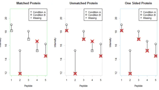
as “matched”, “unmatched”, “one-sided” or “missing”. Figure 3.1 presents a visual depiction.
Missing proteins are proteins for which peptides were identified but no peptide intensities
were observed. These are not interesting and even though they can be estimated with M3, M5 or
KNNQ we recommend just removing them from the study. Matched proteins are proteins that
have at least one matched peptide pair. With at least one shared peptide from each sample,
all of the methods can be used for estimation. An unmatched protein has observed intensities
from each sample but no peptides that are quantified in both samples. One-Sided proteins have
intensities from peptides in only one sample and are completely missing in the other. This can be
indicative of a large fold change difference. M5, M3 and KNNQ can be used to estimate all types
of proteins. The ANOVA model and QRollup can be used for both matched and unmatched
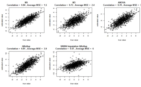
Figure 3.1: The three categories of proteins. Matched proteins contain at least one matched peptide pair. Unmatched proteins contain data from both conditions but no matched pairs. One-sided proteins contain peptide measurements from only one sample.
3.2.3 Simulation Results
The sampling chains all appeared to achieve stationary distributions after about 300 draws
(in the real data this was achieved within 50). For this reason, our estimates were based on the
posterior mean after a burn in length of 500 draws.
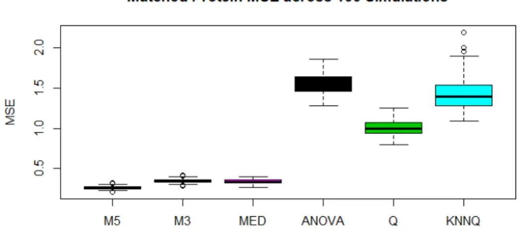
Figure 3.2 shows the distribution of mean squared errors across simulations. The most obvious
result here is that the methods based on ratios are far outperforming methods based on average
intensities. M5 demonstrates the best performance with an average MSE of 0.26. The method
of medians was the second most accurate with an MSE of 0.35, which represents an increase in
error of 35%. This is a fairly large increase but it is hardly noticeable relative to the error coming
from the average intensity methods. The best of these was QRollup with an average MSE of 1,
which represents an increase of 285%. It should be noted that the commonly used validation tool
of correlation does not do a very good job of assessing algorithmic weaknesses here. Figure 3.3
shows that even though some of these methods more than sextuple mean squared error, the
Figure 3.2: MSE for each method computed across matched Proteins and within each simulation.
K-Nearest Neighbors appears to be detrimental to the accuracy of QRollup estimates.
These relationships can be further explored by categorizing proteins according to the
percent-age of peptides which are missing as shown in Figure 3.4. This plot shows that the error for the
KNNQ method increases substantially once more than 50% of the data requires imputation. In
this chart we can see that, as missingness increases, the ANOVA estimation also loses accuracy
at a much faster rate than the other methods. This is likely because the ANOVA model simply
reports average intensities within each sample regardless of the amount of missing data.
In the case of one-sided and unmatched Proteins the method of medians is obviously not
applicable. Among the other methods the rank ordering based on average MSE remains the
same. (see Figure 3.5).
In this case the average MSE for M5 is 1.5 and the second best is the M3 model at 2.4. The
best average intensity method was the ANOVA model with an MSE of 3. Correlation coefficients
are much weaker in this category as pictured in Figure 3.6.
Arguably the greatest advantage to using the M5 model comes from the ability to estimate
Figure 3.3: Scatterplot of true simulated fold changes for matched Proteins vs their estimates across all simulations. Correlation coefficients are also computed across all simulations.
Figure 3.5: MSE for each method computed across unmatched proteins and within each simula-tion. The method of medians, MED, is not applicable to unmatched proteins.
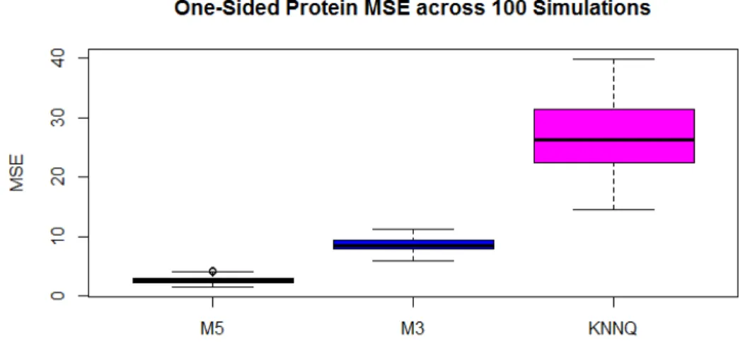
Figure 3.7: MSE for each method computed across One-Sided proteins and within each simulation. The method of medians (MED), ANOVA, and QRollup (Q) are not applicable to One-Sided proteins
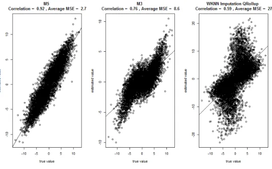
observed values. Keep in mind for a One-Sided protein that we could assume that the abundance
of the missing value is between zero and the detection limit. However, the upper bound on an
abundance ratio is infinite. Nonetheless, M5 does provide decent estimates in this situation as
can be seen in Figure 3.7. Only three methods were capable of estimating one-sided proteins and
only one of them could be considered useful. The MSE’s for M5, M3 and KNNQ were respectively
2.7, 8.6 and 27. The range of the log-scale fold changes in this simulation were roughly -10 to
10. So an average MSE for M5 of 2.7 is certainly small enough for the estimates to be of interest.
The scatter plot in Figure 3.8 strongly highlights the advantages of the M5 model.
3.3 Breast Cancer Data
In order to make sure the results of our simulation study are not artifacts of the data generation
procedure, we also analyzed the effect of non-informative missingness on a real data set. The
data, generated by the Chen Biochemistry Lab, contains peptide level LFQ measurements from
Figure 3.8: Scatter plot of true simulated fold changes for one-sided proteins vs their estimates across all simulations. Correlation coefficients are computed across all simulations.
the supplementary material. 11,866 unique proteins were identified in the data, of these 594 were
Missing, 9,265 had at least one peptide pair, 1,810 were one-sided and 197 had intensities in both
samples but no matched pairs. This breakdown is pictured in Figure 3.9.
Not considering missing proteins, we can see that before we even do an analysis the M5
model is capable of estimating an additional 2,007 (22%) proteins compared with the method of
medians. This would be a substantial gain if our method is capable of estimating those proteins
Figure 3.10: M5 estimates of the log fold change between proteins found in Basal and Luminal breast cancer tissues. Only proteins with 95% credible intervals that do not contain zero are pictured.
with a decent level of accuracy as our simulations suggest. Furthermore, the entire data set
contains information on 248,342 peptides, 61,418 (about 25%) of which are missing. There is a
tremendous amount of information in the patterns of those 61,418 missing values, and in theory
the M5 model takes full advantage of them. M5 model estimates were computed on a random set
of 1,000 proteins and 95% credible regions were computed. 1,000 draws from the Gibbs sampler
were used with a burn in length of 500. We reduced the data size purely for computational
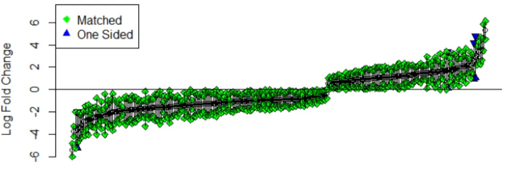
simplicity. From the 1,000 proteins, 252 matched Proteins and 4 one-sided Proteins did not
contain zero in their credible intervals (Figure 3.10). Among the 4 one-sided Proteins is protein
O75363 which is better known as the gene product for the Novel Amplified in Breast Cancer-1
gene (NABC1). This gene is known to be involved in cancer typically being up-regulated in
breast cancers and down-regulated in colon cancer (Beardsley et al., 2003). Since this protein
was one-sided in our dataset no useful information regarding NABC1 would have been found
without the M5 model. After estimation, we computed the square of the M5 estimates divided
by the posterior standard deviation. The proteins were then ranked in descending order and are
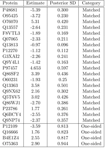
Table 3.3: Twenty proteins ordered by the highest squared ratio of posterior mean to posterior standard error. At the bottom of the table is the complete set of one-sided proteins for which the credible region did not include zero.
Protein Estimate Posterior SD Category
P48681 -5.39 0.300 Matched
O95425 -3.72 0.230 Matched
O76070 5.31 0.420 Matched
Q13557 -2.64 0.231 Matched
F8VTL3 -1.89 0.169 Matched
Q07065 -2.33 0.211 Matched
Q13813 -0.97 0.096 Matched
P12270 -1.12 0.112 Matched
G3XAI2 -2.26 0.241 Matched
Q9Y4L1 -1.42 0.163 Matched
P97457 4.653 0.597 Matched
Q86SF2 3.39 0.436 Matched
O60231 -1.93 0.25 Matched
Q13363 3.58 0.501 Matched
Q9NX62 2.16 0.302 Matched
Q5T6V5 3.02 0.426 Matched
Q86WJ1 -2.70 0.386 Matched
P23786 1.77 0.261 Matched
Q6BCY4 -2.55 0.376 Matched
Q9NP74 -2.37 0.357 Matched
P12109 -3.59 0.813 One-sided
Q16666 1.76 0.823 One-sided
B4E1Z4 2.55 0.817 One-sided
on each of the six estimation methods. To accomplish this goal we first reduce the data to allow
a complete case analysis, so that only peptides with observed intensities from both samples are
included in the reduced dataset. From this complete-case data, 500 proteins were randomly
selected for a sensitivity analysis. The mean peptide ratio within each protein was calculated
and considered to be the reference value. We explored what happens to the estimates from each
model as higher levels of intensity-dependent missingness are introduced. Appropriate values of
the missingness parameter b were discovered by trial and error to provide overall missingness
levels of 1, 5, 10, 20, 30, 40 and 50 percent. Mean squared error was then calculated for each of
the six methods on all 7 datasets.
3.3.1 Results of the Sensitivity Analysis
We explored the effect of intensity dependent missingness on complete case estimates. The
performance demonstrated similar patterns to what we found in the simulation analysis with
ratio based methods having far more stable estimates than the average intensity based methods,
shown in Figure 3.11.
These plots paint a picture consistent with the results from the simulation study. The M5
model outperforms all other methods. The method of median ratios and the M3 model have
very similar performance. The ANOVA model and QRollup methods perform comparably to
the ratio-based methods until the missingness is increased to around 10%. Once missingness hits
40%, the difference in frameworks becomes substantial, and at 50% the average MSE from KNNQ
is about eleven times higher than that from the M5 model.
3.4 Misspecification of the Missing Data Mechanism
An obvious artificial strength of the simulation study is the use of the same missing data
mechanism in both the simulation and the analysis. The scientific process supports the use of
a missing data mechanism in which the probability of a peptide being observed is a monotone
Figure 3.11: MSE computed as the average squared difference between the estimate from a complete case analysis and the estimate from a dataset with simulated intensity dependent miss-ingness. MSE for QRollup with weighted KNN imputation takes the values 2.34 and 3.31 at 40 and 50 percent missingness respectively. These values were too extreme to be plotted with the other methods.
suggest the proper shape of this curve. Our probit model fits the monotonicity requirement
however it is not unique in doing so. To examine the robustness to misspecification of the missing
data mechanism we compare estimation results from three different missing data mechanisms; a
linear model within a probit function, a quadratic model within a probit function and a linear
model within a logit function. Data was simulated 100 times and for each data set a different set
of missing values was simulated according to the three different models. Simulation parameters
were selected so that the overall percentage of missing values would be near 33%. As pictured
in Figure 3.12, the results suggest that the M5 model is fairly robust to misspecification of the
missing data mechanism. Amongst matched proteins the worst case scenario occurred when the
real mechanism was a logit model. In this case the average MSE increased by 8% from .26 to .28,
which is still 20% lower than the MSE for the method of medians found in the simulation study.
Misspecification from a quadratic model actually reduced the average MSE by 10%. These results
seem to suggest that sharper the increase in the probability of observing a peptide the better
Figure 3.12: MSE computed from 100 simulations utilizing 3 different missing data mechanisms.
were more pronounced. For one-sided proteins we observed a 42% increase in average MSE
with a probit misspecification and a 34% decrease for the quadratic model. For unmatched
proteins these changes were 43% and -53% respectively. The increased effect of the missing data
mechanism for these proteins should not be surprising since the mechanism plays a larger role in
the estimation when no matched pairs are observed. In the worst case scenario the average MSE
for a one-sided Protein from a logit missing data model was 3.87. With a range of fold changes
in the data from roughly -10 to 10 an MSE of 3.87 is highly encouraging as it suggests that even
with misspecification the M5 model provides a legitimate way to detect one-sided proteins with
large fold changes.
3.5 Conclusion
We have identified the two fundamental statistical features of mass spectrometry proteomics
as matched pairs data and non-ignorable missingness. Of the two features, ignoring matched pairs
appears to be far more detrimental than ignoring the missing data bias. Not only is the average
intensity across peptides difficult to interpret, but the simple method of taking the median ratio
greatly outperforms methods based on average intensities in terms of mean squared error. In
turn, relative to the method of medians, our M5 model is capable of improving both the depth