CAS: Multivariate Copulas for Financial Modeling

Modeling

by Gary Venter, Jack Barnett, Rodney Kreps, and John Major

ABSTRACT

Although the copula literature has many instances of

bi-variate copulas, once more than two bi-variates are correl ated,

the choice of copulas often comes down to selection of the

degrees-of-freedom parameter in the

t

-copula. In search for

a wider selection of multivariate copulas we review a

gen-eralization of the

t

-copula and some copulas defined by

Harry Joe. Generalizing the

t

-copula gives more flexibility

in setting tail behavior. Possible applications include

in-surance losses by line, credit risk by issuer, and exchange

rates. The Joe copulas are somewhat restricted in the range

of correlations and tail dependencies that can be produced.

However, both right- and left-positive tail dependence is

possible, and the behavior is somewhat different from the

t

-copula.

KEYWORDS

1. Introduction

Copulas provide a convenient way to express multivariate distributions. Given the individual distribution functionsF_i(X_i) the multivariate dis-tribution can be expressed as a copula function applied to the probabilities, i.e., F(X₁,: : :,X_n) = C[F₁(X₁),: : :,F_n(X_n)]. Venter [6] discusses many of the basic issues of using copulas with the heavy-tailed distributions of property and liabil-ity (P&L) insurance. One of the key concepts is that copulas can control where in the range of probabilities the dependence is strongest. Any copulaCis itself a multivariate distribution func-tion but one that applies only to uniform distribu-tions on the unit square, unit cube,: : :, depending on dimension. The uniform [0, 1] variables are interpreted as probabilities from other distribu-tions and are represented byU, V, etc.

One application is correlation in losses across lines of business. Lines tend to be weakly related in most cases but can be strongly cor-related in extreme cases, like earthquakes. Belguise and Levi [1] study copulas applied to catastrophe losses across lines. With financial modeling growing in importance, other poten-tial applications of copulas in insurance com-pany management include the modeling of de-pendence between loss and loss expense, depen-dence among asset classes, dependepen-dence among currency exchange rates, and credit risk among reinsurers.

The upper and lower tail dependence coeffi-cients of a copula provide quantification of tail strength. These can be defined using the right and left tail concentration functionsR and L on (0, 1):

R(z) = Pr(U > zjV > z) and

L(z) = Pr(U < zjV < z):

The upper tail dependence coefficient is the limit ofR asz_!1, and the lower tail dependence

co-efficient is the limit of L asz_!0. For the nor-mal copula and many others, these coefficients are zero. This means that for extreme values the distributions are uncorrelated, so large-large or small-small combinations are not likely. How-ever, this is somewhat misleading, as the slopes of the R and L functions for the normal and t-copulas can be very steep near the limits. Thus there can be a significant degree of de-pendence near the limits even when it is zero at the limit. Thus looking atR(z) forz a bit less than 1 may be the best way to examine large loss dependencies.

While a variety of bivariate copulas is avail-able, when more than two variables are involved the practical choice comes down to normal vs. t-copula. The normal copula is essentially the t-copula with high degrees of freedom (df), so the choice is basically what df to use in that cop-ula. Venter [5] discusses the use of the t-copula in insurance. The t takes a correlation param-eter for each pair of variates, and any correla-tion matrix can be used. The df parameter adds a common-shock effect. This can be seen in the simulation methodology, where first a vector of multivariate normal deviates is simulated then the vector is multiplied by a draw from a sin-gle inverse gamma distribution. The df parameter is the shape parameter of the latter distribution, which is more heavy-tailed with lower df. The factor drawn represents a common shock that hits all the normal variates with the same fac-tor. This increases tail dependence in both the right and left tails but also increases the like-lihood of anti-correlated results, so the overall correlation stays the same as in the normal copula.

little effect on risk measurement overall, which is largely affected by the right tail. The single df parameter is more of a restriction. It results in giving more tail dependence to more strongly correlated pairs. This is reasonable but is not al-ways consistent with data.

Thus more flexible multivariate copulas would be useful. One alternative provided by Daul et al. [2] is the groupedt-copula, which uses

differ-ent df parameters for differdiffer-ent subgroups of vari-ables, such as corporate bonds grouped by coun-try. We introduce a special case of that called the individuated t-copula, or IT, which has a df

parameter for each variable. Another direction is that of Joe [3], who develops a method for combining simple copulas to build up multivari-ate copulas. Three of these–called MM1, MM2, and MM3–have closed-form expressions. We investigate some of the properties of these copulas.

The t-copula for n variates has (n2¡n+ 2)=2

parameters. The MMC copulas have one more parameter for each variate and so have (n2+n+

2)=2 all together, while the IT has (n2+n)=2.

This situation does not include enough parame-ters to have separate control of the strength of the tail dependency for every pair of variates, but it does add some flexibility. The IT copula generalizes the t so it can be tried any time the t is too limiting in the possibilities for tail be-havior. The MMC copulas have a parameter for each pair of variates, but this does not give them full flexibility in matching a covariance matrix. When all the bivariate correlations are fairly low (below 50% in the trivariate case but decreasing with more dimensions) they can usually all be matched, but the higher they get the more simi-lar they are forced to be. This would probably be fine for insurance losses by line of business, as they tend to have low correlations overall but can be related when the losses are large. In modeling them, some additional flexibility in tail behavior

vs. overall correlation could be helpful, so this could be an application where the MMC copulas would have an advantage over the t-copula.

2. IT copula

This copula is most readily described by the simulation procedure from its parameters, which are a correlation matrix½and a parameterºn for

each of the N variables. The simulation starts with the generation of a multivariate normal vec-tor fzng with correlation matrix ½ by the usual

approach (Cholesky decomposition, etc.). Then a uniform (0, 1) variate u is drawn. The inverse chi-squared distribution quantile with probability uand dfºn, denoted bywn=hn(u), is calculated.

Thentn=zn[ºn=wn]1=2 ist-distributed withºndf.

To get the copula value, which is a probability, thatt-distribution is applied totn. The only

differ-ence between this and simulation of the t-copula

is thetuses the same inverse chi-square draw for each variate.

The chi-squared distribution is a special case of the gamma. The ratio wn=ºn is a scale

trans-form of the chi-squared variate, so is a gamma variate. If the gamma density is parameterized to be proportional to x®_¡1e_¡x=¯, then wn=ºn

has parameters ¯= 2=ºn and ®=ºn=2. This is

a distribution with mean 1. It can be simulated easily if an inverse gamma function is available, as in some spreadsheets. It is not necessary for the df to be an integer for this to work. If not an integer, a beta distribution can be used to calculate the t-distribution probability, as in

Venter [5].

Although the simulation is straightforward, the copula density and probability functions are somewhat complicated. In terms of hn, the

density at (u1,: : :,un) can be shown to be: c(~u) = Z 1 0 QN n=1 8 < : p

h_n(y)¡(ºn=2) Ã

1 + t 2 n º_n

!(1+ºn)=2, ¡

µ 1 +º_n

2 ¶9₌

;

p

det(½)(2¼)N_exp Ã

P n,m

J_n,mt_nt_m 2

s

h_n(y)hm(y) º_nº_m

! dy:

This has to be computed numerically unless the df parameters are all the same, in which case it reduces to thet-copula density.

Daul et al. [2] find that the correlations (Spear-man’s rho and Kendall’s tau) are not exactly the same as for thet-copula, but are quite close. Also the bivariate t-copula right and left dependence coefficients are S_n+1f[(n+ 1)(1¡½)=(1 +½)]0:5g

whereS_n+1is the t-distribution survival function (PrX > x) withn+ 1 df. If we denote the bivari-ate standard normal survival function as S(x,y) = Pr(X > x,Y > y), then the tail dependence coefficients for X_m and X_n for the IT copula are:

Z ₁

0 S(cn y1=ºn_,c

my1=ºm)dy,

where c_j=p2 "

¡ Ã

1 +º_j 2

! ,_p 4¼

#1=ºj :

These tend to be between the t-copula depen-dence coefficients for the two dfs but closer to that for the higher of the two dfs if these are very different.

Fitting the IT by maximum likelihood is possi-ble but involves several numerical steps. Alterna-tively, the df parameter for the t-copula could be estimated for each pair of variables by matching tail behavior, as in Venter [5], and then individ-ual dfs assigned to be consistent with this. Daul et al. [2] propose separate t-copulas for different groups of variables, which are combined into a single copula with the overall correlation matrix and the separate dfs.

3. MMC copulas

Joe’s MM1, MM2, and MM3 copulas each have an overall strength parameter µ, a param-eter for each pair of variables ±_ij (not the Kro-necker delta), and add an additional parameter p_j, with 1=pj¸m¡1, for each of themvariables U_j, which gives the possibility of more control over the tails.

The parameters are then±_ijfori < j,p_j, forj= 1,: : :,m, and µ. For each variableu_j, it is conve-nient to use the abbreviationsy_j= (¡lnu_j)µ and w_j=p_j(u¡_jµ¡1). The±_ij parameters would seem to allow for a correlation matrix, but it turns out that there are restrictions on how different the correlations can be, with the µ parameter exert-ing a lot of control. In effect, the parameters do not have as much freedom to fit to data as might be desired. The copula functions and dependency coefficients are given below. The density func-tions for the copulas needed for maximum like-lihood estimation (MLE) are discussed in Ap-pendix 1. ApAp-pendix 2 discusses numerical eval-uation of MLE and rejection sampling (Tillé [4]) as a method for assessing standard errors.

MM1

Here ±_{ij ¸}1 and µ_¸1. The copula at the m-vectoruis:

C(u) = exp 8 < :¡ 2 4 m X j=1

(1_¡(m_¡1)p_j)y_j

+X i<j

((p_iy_i)±ij_{+ (p}

jyj)±ij)1=±ij 3 5

The bivariate i,j margin is:

C(ui,uj) = expf¡[(1¡pi)yi+ (1¡pj)yj

+ ((piyi)±ij+ (pjyj)±ij)1=±ij]1=µg

Lower tail dependence is zero. Upper tail depen-dence is given by:

¸ij = 2¡[2 + (p±_iij+p_j±ij)1=±ij¡pi¡pj]1=µ

MM2

Here ±ij>0 and µ >0. The copula at the m

-vector uis: C(u) =

2 4

m X

j=1

u¡_jµ+ 1¡m

¡X

i<j

(w_i¡±ij+w_j¡±ij)¡1=±ij

3 5¡

1=µ

The i,j margin is:

C(ui,uj) = [u¡_i µ+u¡_jµ¡1

¡(w¡_i ±ij+w_j¡±ij)¡1=±ij]¡1=µ

Because both upper and lower tail dependence are positive for this copula, a subscript is used to distinguish them here. The upper tail dependence is:

¸ij,U= (p¡_i ±ij+p¡_j±ij)¡1=±ij

The lower tail dependence is:

¸ij,L= [2¡(p¡_i ±ij+p¡_j±ij)¡1=±ij]¡1=µ

MM3

This starts with ±ij >0 and µ >1 (Although

Joe saysµ >0 is allowed, we have had problems

ifµ <1.). The copula atuis C(u) = exp

(¡" _m X

j=1

yj¡X i<j

((piyi)_¡±ij

+ (pjyj)¡±ij)¡1=±ij

#1=µ)

The i,j margin is

C(ui,uj) = expf¡[yi+yj¡((piyi)_¡±ij

+ (pjyj)¡±ij)¡1=±ij]1=µg

The upper tail dependence is:

¸ij= 2¡[2¡(p_¡i ±ij+p_¡j±ij)_¡1=±ij]1=µ

4. Range of possible correlations

and dependencies

It turns out that not every possible correlation matrix can be matched by these copulas. The µ

parameter determines a lot of what is possible for each copula. Tables 1—6 show the tail depen-dence and Spearman’s½for selected parameters. For MM1 and MM3 the lower tail dependence is zero, so it is not shown. It is shown for MM2, but there the upper dependence does not depend on µ, so “any” is shown forµ.

5. Discussion

The tables in the previous section are bivariate relationships. However, since the p parameters can be no greater than 1=(m_¡1), the possible

values of p, and so the range of possible

corre-lations and tail dependencies, reduce as the di-mension increases. The µ parameter i n general

has a great deal of influence over what any of these copulas can do. As µgets higher, the other parameters have very little influence. Thus when it is high, all pairs of variables will have simi-lar correlations and tail dependencies. This is the case for any of the correlation coefficients (lin-ear, rank, tau) so we use the term “correlation” generically. When µ is low, however, it is not

Table 1. MM1 upper tail dependence

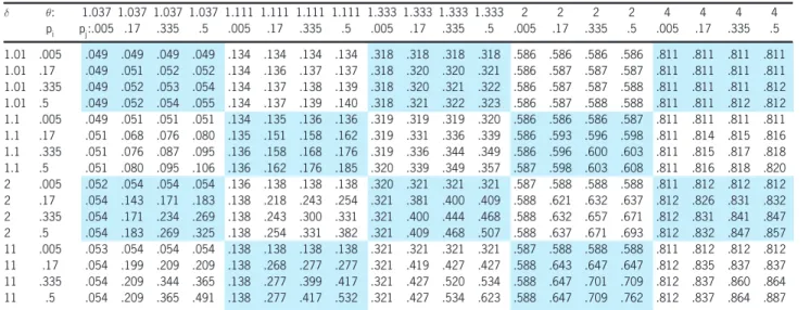
± µ: 1.037 1.037 1.037 1.037 1.111 1.111 1.111 1.111 1.333 1.333 1.333 1.333 2 2 2 2 4 4 4 4

p_i p_j:.005 .17 .335 .5 .005 .17 .335 .5 .005 .17 .335 .5 .005 .17 .335 .5 .005 .17 .335 .5

1.01 .005 .049 .049 .049 .049 .134 .134 .134 .134 .318 .318 .318 .318 .586 .586 .586 .586 .811 .811 .811 .811 1.01 .17 .049 .051 .052 .052 .134 .136 .137 .137 .318 .320 .320 .321 .586 .587 .587 .587 .811 .811 .811 .811 1.01 .335 .049 .052 .053 .054 .134 .137 .138 .139 .318 .320 .321 .322 .586 .587 .587 .588 .811 .811 .811 .812 1.01 .5 .049 .052 .054 .055 .134 .137 .139 .140 .318 .321 .322 .323 .586 .587 .588 .588 .811 .811 .812 .812 1.1 .005 .049 .051 .051 .051 .134 .135 .136 .136 .319 .319 .319 .320 .586 .586 .586 .587 .811 .811 .811 .811 1.1 .17 .051 .068 .076 .080 .135 .151 .158 .162 .319 .331 .336 .339 .586 .593 .596 .598 .811 .814 .815 .816 1.1 .335 .051 .076 .087 .095 .136 .158 .168 .176 .319 .336 .344 .349 .586 .596 .600 .603 .811 .815 .817 .818 1.1 .5 .051 .080 .095 .106 .136 .162 .176 .185 .320 .339 .349 .357 .587 .598 .603 .608 .811 .816 .818 .820 2 .005 .052 .054 .054 .054 .136 .138 .138 .138 .320 .321 .321 .321 .587 .588 .588 .588 .811 .812 .812 .812 2 .17 .054 .143 .171 .183 .138 .218 .243 .254 .321 .381 .400 .409 .588 .621 .632 .637 .812 .826 .831 .832 2 .335 .054 .171 .234 .269 .138 .243 .300 .331 .321 .400 .444 .468 .588 .632 .657 .671 .812 .831 .841 .847 2 .5 .054 .183 .269 .325 .138 .254 .331 .382 .321 .409 .468 .507 .588 .637 .671 .693 .812 .832 .847 .857 11 .005 .053 .054 .054 .054 .138 .138 .138 .138 .321 .321 .321 .321 .587 .588 .588 .588 .811 .812 .812 .812 11 .17 .054 .199 .209 .209 .138 .268 .277 .277 .321 .419 .427 .427 .588 .643 .647 .647 .812 .835 .837 .837 11 .335 .054 .209 .344 .365 .138 .277 .399 .417 .321 .427 .520 .534 .588 .647 .701 .709 .812 .837 .860 .864 11 .5 .054 .209 .365 .491 .138 .277 .417 .532 .321 .427 .534 .623 .588 .647 .709 .762 .812 .837 .864 .887

Table 2. MM1 Spearman’s½

± µ: 1.037 1.037 1.037 1.037 1.111 1.111 1.111 1.111 1.333 1.333 1.333 1.333 2 2 2 2 4 4 4 4

p_i p_j:.005 .17 .335 .5 .005 .17 .335 .5 .005 .17 .335 .5 .005 .17 .335 .5 .005 .17 .335 .5

1.01 .01 .053 .054 .054 .054 .149 .149 .149 .149 .364 .364 .364 .364 .682 .682 .682 .682 .913 .913 .913 .913 1.01 .17 .054 .056 .057 .057 .149 .151 .152 .152 .364 .365 .366 .366 .682 .683 .684 .684 .913 .913 .913 .913 1.01 .335 .054 .057 .058 .059 .149 .152 .153 .154 .364 .366 .367 .368 .682 .684 .684 .685 .913 .913 .913 .913 1.01 .5 .054 .057 .059 .061 .149 .152 .154 .155 .364 .366 .368 .369 .682 .684 .685 .685 .913 .913 .913 .913 1.1 .01 .054 .056 .056 .056 .149 .151 .151 .151 .364 .365 .365 .366 .682 .683 .683 .683 .913 .913 .913 .913 1.1 .17 .056 .075 .083 .088 .151 .168 .176 .181 .365 .379 .385 .389 .683 .691 .694 .696 .913 .915 .916 .917 1.1 .335 .056 .083 .096 .105 .151 .176 .187 .196 .365 .385 .394 .401 .683 .694 .699 .702 .913 .916 .917 .918 1.1 .5 .056 .088 .105 .117 .151 .181 .196 .207 .366 .389 .401 .409 .683 .696 .702 .707 .913 .917 .918 .920 2 .01 .056 .060 .060 .060 .151 .155 .155 .155 .366 .369 .369 .369 .683 .685 .685 .686 .913 .913 .914 .914 2 .17 .060 .148 .182 .203 .155 .235 .267 .286 .369 .430 .455 .470 .685 .717 .730 .739 .913 .923 .926 .929 2 .335 .060 .182 .245 .287 .155 .267 .324 .362 .369 .455 .498 .528 .685 .730 .753 .768 .914 .926 .933 .937 2 .5 .060 .203 .287 .348 .155 .286 .362 .417 .369 .470 .528 .570 .686 .739 .768 .790 .914 .929 .937 .943 11 .01 .057 .060 .061 .061 .152 .155 .155 .155 .366 .369 .369 .369 .684 .686 .686 .686 .913 .914 .914 .914 11 .17 .060 .179 .223 .246 .155 .263 .303 .325 .369 .451 .482 .500 .686 .727 .744 .754 .914 .925 .930 .933 11 .335 .061 .223 .312 .369 .155 .303 .383 .435 .369 .482 .542 .582 .686 .744 .774 .794 .914 .930 .938 .944 11 .5 .061 .246 .369 .457 .155 .325 .435 .514 .369 .500 .582 .641 .686 .754 .794 .823 .914 .933 .944 .952

Table 3. MM2 upper tail dependence and MM2 lower tail dependence

MM2 Upper Tail Dependence MM2 Lower Tail Dependence

± µ: any any any any .111 .111 .111 .111 .333 .333 .333 .333 1 1 1 1 3 3 3 3

p_i p_j:.005 .17 .335 .5 .005 .17 .335 .5 .005 .17 .335 .5 .005 .17 .335 .5 .005 .17 .335 .5

Table 4. MM2 Spearman’s½

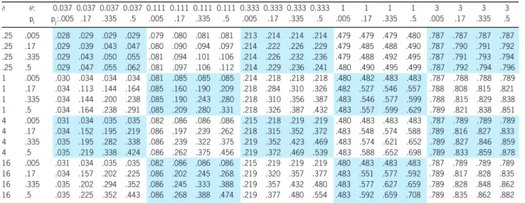
± µ: 0.037 0.037 0.037 0.037 0.111 0.111 0.111 0.111 0.333 0.333 0.333 0.333 1 1 1 1 3 3 3 3

p_i p_j:.005 .17 .335 .5 .005 .17 .335 .5 .005 .17 .335 .5 .005 .17 .335 .5 .005 .17 .335 .5

.25 .005 .028 .029 .029 .029 .079 .080 .081 .081 .213 .214 .214 .214 .479 .479 .479 .480 .787 .787 .787 .787 .25 .17 .029 .039 .043 .047 .080 .090 .094 .097 .214 .222 .226 .229 .479 .485 .488 .490 .787 .790 .791 .792 .25 .335 .029 .043 .050 .055 .081 .094 .101 .106 .214 .226 .232 .236 .479 .488 .492 .495 .787 .791 .793 .794 .25 .5 .029 .047 .055 .062 .081 .097 .106 .112 .214 .229 .236 .241 .480 .490 .495 .499 .787 .792 .794 .796 1 .005 .030 .034 .034 .034 .081 .085 .085 .085 .214 .218 .218 .218 .480 .482 .483 .483 .787 .788 .788 .789 1 .17 .034 .113 .144 .164 .085 .160 .190 .209 .218 .284 .310 .326 .482 .527 .546 .557 .788 .808 .815 .821 1 .335 .034 .144 .200 .238 .085 .190 .243 .280 .218 .310 .356 .387 .483 .546 .577 .599 .788 .815 .829 .838 1 .5 .034 .164 .238 .291 .085 .209 .280 .331 .218 .326 .387 .432 .483 .557 .599 .629 .789 .821 .838 .851 4 .005 .031 .034 .035 .035 .082 .086 .086 .086 .215 .218 .219 .219 .480 .483 .483 .483 .787 .789 .789 .789 4 .17 .034 .152 .195 .219 .086 .197 .239 .262 .218 .315 .352 .372 .483 .548 .574 .588 .789 .816 .827 .833 4 .335 .035 .195 .282 .338 .086 .239 .322 .375 .219 .352 .423 .469 .483 .574 .621 .652 .789 .827 .846 .859 4 .5 .035 .219 .338 .424 .086 .262 .375 .456 .219 .372 .469 .539 .483 .588 .652 .698 .789 .833 .859 .878 16 .005 .031 .034 .035 .035 .082 .086 .086 .086 .215 .219 .219 .219 .480 .483 .483 .483 .787 .789 .789 .789 16 .17 .034 .157 .202 .225 .086 .202 .245 .268 .219 .320 .357 .377 .483 .551 .577 .592 .789 .817 .828 .835 16 .335 .035 .202 .294 .352 .086 .245 .333 .388 .219 .357 .432 .480 .483 .577 .627 .659 .789 .828 .848 .862 16 .5 .035 .225 .352 .443 .086 .268 .388 .474 .219 .377 .480 .554 .483 .592 .659 .708 .789 .835 .862 .882

Table 5. MM3 upper tail dependence

± µ: 1.037 1.037 1.037 1.037 1.111 1.111 1.111 1.111 1.333 1.333 1.333 1.333 2 2 2 2 4 4 4 4

p_i p_j:.005 .17 .335 .5 .005 .17 .335 .5 .005 .17 .335 .5 .005 .17 .335 .5 .005 .17 .335 .5

.25 .005 .049 .050 .050 .050 .134 .135 .135 .135 .318 .319 .319 .319 .586 .586 .586 .586 .811 .811 .811 .811 .25 .17 .050 .059 .063 .065 .135 .143 .146 .149 .319 .325 .327 .329 .586 .590 .591 .592 .811 .812 .813 .813 .25 .335 .050 .063 .069 .073 .135 .146 .152 .155 .319 .327 .331 .334 .586 .591 .593 .595 .811 .813 .814 .815 .25 .5 .050 .065 .073 .078 .135 .149 .155 .160 .319 .329 .334 .338 .586 .592 .595 .597 .811 .813 .815 .815 1 .005 .051 .053 .054 .054 .136 .138 .138 .138 .320 .321 .321 .321 .587 .588 .588 .588 .811 .812 .812 .812 1 .17 .053 .129 .155 .168 .138 .205 .229 .241 .321 .372 .390 .399 .588 .616 .626 .631 .812 .824 .828 .830 1 .335 .054 .155 .207 .238 .138 .229 .275 .303 .321 .390 .425 .446 .588 .626 .646 .659 .812 .828 .837 .842 1 .5 .054 .168 .238 .285 .138 .241 .303 .345 .321 .399 .446 .478 .588 .631 .659 .677 .812 .830 .842 .850 4 .005 .053 .054 .054 .054 .137 .138 .138 .138 .321 .321 .321 .321 .587 .588 .588 .588 .811 .812 .812 .812 4 .17 .054 .184 .207 .209 .138 .254 .275 .277 .321 .409 .425 .426 .588 .637 .646 .647 .812 .833 .836 .837 4 .335 .054 .207 .315 .351 .138 .275 .372 .405 .321 .425 .499 .524 .588 .646 .689 .704 .812 .836 .855 .862 4 .5 .054 .209 .351 .446 .138 .277 .405 .491 .321 .426 .524 .591 .588 .647 .704 .743 .812 .837 .862 .879 16 .005 .053 .054 .054 .054 .138 .138 .138 .138 .321 .321 .321 .321 .587 .588 .588 .588 .812 .812 .812 .812 16 .17 .054 .202 .209 .209 .138 .271 .277 .277 .321 .422 .427 .427 .588 .645 .647 .647 .812 .836 .837 .837 16 .335 .054 .209 .352 .365 .138 .277 .406 .418 .321 .427 .525 .534 .588 .647 .704 .710 .812 .837 .862 .864 16 .5 .054 .209 .365 .501 .138 .277 .418 .541 .321 .427 .534 .630 .588 .647 .710 .767 .812 .837 .864 .889

Table 6. MM3 Spearman’s½

± µ: 1.037 1.037 1.037 1.037 1.111 1.111 1.111 1.111 1.333 1.333 1.333 1.333 2 2 2 2 4 4 4 4

p_i p_j:.005 .17 .335 .5 .005 .17 .335 .5 .005 .17 .335 .5 .005 .17 .335 .5 .005 .17 .335 .5

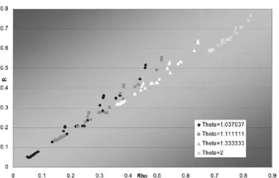
Figure 1. MM1Ras a function of rho by theta,m= 3

Figure 2. MM2Ras a function of rho by theta,m= 3

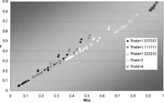
Also the right tail dependenceR and the corre-lation are closely related. Scatter plots of R as a function of ½for different values of µare shown for the cases m= 3 and m= 7 for the MM1 and MM2 copulas and m= 7 for MM3 in Figures 1—5. These points are taken from the above ta-bles so just give a suggestion of the spread in

Figure 3. MM1Ras a function of rho by theta,m= 7

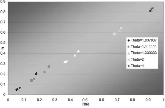
Figure 4. MM2Ras a function of rho by theta,m= 7

For MM2,R is not a function of µ, so a wider range of Rs is possible for any µ. The possi-ble range of ½ for each µ is about the same for each copula. This range decreases with higher ms, however, due to the restricted range of p.

The relationship for MM3 in Figure 5 is simi-lar to that for MM1 in Figure 1, but MM3 might have a bit more possible spread in R.

6. Fitting MM1 and MM2

Table 7. Parameters for the various fitting methods

MM2 MM1 t

SSE MLE bi SSE MLE bi MLE tri MLE bi MLE tri

±₁₂ 2.62588 1.50608 3.69513 2.14275 2.1094 0.491 0.490

±₁₃ 0.80055 0.43963 1.52005 1.19832 1.1152 0.262 0.266

±₂₃ 3.2E-07 0.0103 1 1 1 0.097 0.097

p₁ 0.49881 0.37649 0.49963 0.40533 0.37175

p₂ 0.5 0.5 0.5 0.5 0.5

p₃ 0.26236 0.49625 0.29097 0.5 0.5

µ 0.19599 0.2209 1.08308 1.0939 1.1234 20.53 20.95

Figure 5. MM2Ras a function of rho by theta,m= 3

illustrated, as can fitting methods. The data con-sists of monthly changes in the US $ exchange rate for the Swedish, Japanese and Canadian cur-rencies from 1971 through September 2005. The data come from the Fred database of the St. Louis Federal Reserve. The Fred exchange rates were converted to monthly change factors, with a fac-tor greater than 1.0 representing an appreciation of the US $ compared to that currency. These factors are comparative movements against the dollar, so if an event strengthens or weakens the dollar in particular, all the currencies would be expected to move in the same direction. Thus there could be common shocks.

The MMC copula densities get increasingly difficult to calculate as the dimension increases.

For this reason, some alternatives to MLE were explored. One alternative is to maximize the product of the bivariate likelihood functions, which just requires the bivariate densities. Since the copulas are defined by the copula functions, an even easier fit is to minimize the distance be-tween the empirical and fitted copulas, measured by sum of squared errors (SSE). Numerical dif-ferentiation, as discussed in Appendix 2, is an-other way to calculate the multivariate MLE but was not tried here.

max-Figure 6. Sweden—JapanJ function

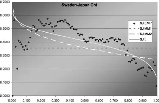
Figure 7. Sweden—JapanÂfunction

ima for both likelihood functions, so we cannot be absolutely sure that these are the global max-ima. Only the bivariate estimates were done for MM2. The SSE parameters are quite a bit dif-ferent from the MLEs. Thus, the product of the bivariate MLEs appears to be the more promising short-cut method.

Figure 8. Sweden—CanadaJ function

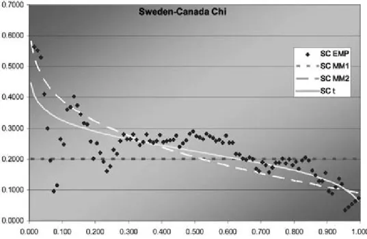
Figure 9. Sweden—CanadaÂfunction

are defined as:

J(z) =_¡z2+ 4 Z z

0 Z z

0

C(u,v)c(u,v)dv du=C(z,z) and

Â(z) = 2_¡ln[C(z,z)]=lnz:

Asz_!1 these approach Kendall’s¿ and the up-per tail dependence R, respectively. They also

can be compared to see the fit in the left tail, which is important for currency movements.

Figure 10. Japan—CanadaJfunction

Figure 11. Japan—CanadaÂfunction

graph, each of the three is best in some range but MM1 is probably best. Overall, MM2 seems to provide almost as good a fit as t, but not quite.

Although this data set is fit best by thet-copula, that does not negate the value of having more than one multivariate copula available. The

re-ciprocals of the factors are of interest and could have the same distribution.

7. Summary

The IT copula has potential for better fits when thet-copula tails differ. Trying to fit this to some actual data seems worthwhile.

The closed-form MMC copulas do not give full flexibility in the range of the bivariate cor-relations that can occur in a single multivariate copula. These copulas would be most appropri-ate when the empirical correlations are all fairly small or fairly close to each other. This gets more so as the number of dimensions increases. These copulas all have somewhat different shapes, and differ from the t-copula as well, so they could be useful with the right data. An interesting ap-plication may be to insurance losses by line of business, as their correlations are all relatively low and the tail dependences may not have the t-copula property of strictly growing with corre-lation. The correlations of losses across lines may not have the t’s symmetric right and left tails ei-ther, but this is less of a concern, as putting too much correlation into small losses is not likely to critically affect the properties of the distribution of the sum of the lines.

Joe also defines MM4 and MM5 copulas. These do not have closed-form expressions, but he asserts that they have a wide range of possi-ble dependence. To build a larger repertoire of multivariate copulas, it may be worth developing algorithms for calculation and fitting these and trying them on live data.

Appendix 1. MMC density

functions

For maximum likelihood estimation, it would be desirable to have expressions for the copula densities, which are mixed partial derivatives of

the copula C functions. Although it is difficult to write down general formulas for the densities, some broad outlines can be developed. Recall the product formula for derivatives (ab)0=a0b+ b0a. Then (abc)0= (ab)0c+abc0=a0bc+ab0c+ abc0. Similarly (abcd)0=a0bcd+ab0cd+abc0d+ abcd0, etc. For any function F of the vector u, consider the simple multivariate functionB(u) = F(u)a_{. Denoting partial derivatives with respect} to the elements ofuby subscripts, we have suc-cessively:

B=Fa:

B_i=aFa¡1F_i:

B_ij=a(a¡1)Fa¡2F_iF_j+aFa¡1F_ij:

B_ijk=a(a¡1)(a¡2)Fa¡3F_iF_jF_k+a(a¡1)Fa¡2

£(F_iF_jk+F_jF_ik+F_kF_ij) +aFa¡1F_ijk:

B_ijkl=a(a¡1)(a¡2)(a¡3)Fa¡4F_iF_jF_kF_l

+a(a¡1)(a¡2)Fa¡3(FijFkFl+FikFjFl

+F_ilF_jF_k+F_jkF_iF_l+F_jlF_iF_k+F_klF_iF_j)

+a(a¡1)Fa¡2(F_iF_jkl+F_jF_ikl+F_kF_ijl

+F_lF_ijk+F_ijF_kl+F_ikF_jl+F_ilF_jk)

+aFa¡1F_ijkl:

This is the form of the MM2 C function. Al-though a pattern is emerging in the subscripts, it seems difficult to write down a general rule for an arbitrary mixed partial.

A similar exercise can be carried out for C(u) =e¡B(u).

C=e¡B:

C₁=¡CB₁:

C₁₂=C(B1B2¡B12):

C₁₂₃=C(B1B23+B2B13+B3B12¡B1B2B3

C₁₂₃₄=C(B1B234+B2B134+B3B124+B4B123

+B₁₂B₃₄+B₁₃B₂₄+B₁₄B₂₃

¡B₁₂B₃B_4¡B₁₃B₂B_4¡B₁₄B₂B₃

¡B₂₃B₁B_4¡B₂₄B₁B_3¡B₃₄B₁B₂

+B₁B₂B₃B_4¡B₁₂₃₄):

This is the form of the MM1 and MM3 C with Fa replacing B.

To calculate the derivatives let x_j=y0_j= µ(¡lnu_j)µ¡1_=u

j, and tj=w0j=µpju¡jµ¡1. The case m= 3 is not too bad. First for MM1:

F(u) = 3 X

j=1

(1_¡2p_j)y_j+X i<j

((p_iy_i)±ij_{+ (p} jyj)

±_ij )1=±ij

Taking the first derivative:

F_i(u) = (1¡2pj)yjxi+ (piyi) ±_ij¡1

p_ix_i

£X

j6=i

((piyi)±ij+ (pjyj)±ij)1=±ij¡1

This would be almost the same for the bivariate margin. Then:

F_ij(u) = (1¡±_ij)(p_ip_jy_iy_j)±ij¡1_p ipjxixj

£((piyi) ±_ij

+ (pjyj) ±_ij

)1=±ij¡2

This is the same for the bivariate margin. From this it is clear thatF₁₂₃= 0. Then taking a= 1=µ and plugging in these values of F_i and F_ij will give all values of B_i, B_ij, and B₁₂₃, which can then be plugged in the formula for C₁₂₃ to give the density. From the formulas forC₁₂the bivari-ate density is similar.

MM2 is even easier, as theC formulas are not needed. What is needed is:

F(u) = 3 X

j=1

u¡_jµ_¡2¡X

i<j (w¡±ij

i +w

¡±_ij j )¡

1=±_ij

This gives:

F_i(u) =_¡µu_i¡µ¡1_¡w¡±ij¡1 i ti

X

j6=i (w¡±ij

i +w ¡±_ij j )¡

1=±_ij¡1

And:

F_ij(u) =_¡(1 +±_ij)(w_iw_j)¡±ij¡1t itj(w

¡±_ij i +w

¡±_ij j )¡

1=±_ij¡2

Again F₁₂₃= 0. Then setting a=¡1=µ gives B₁₂₃, which is the density.

This gets harder and harder as the dimension ofuincreases. Then numerical differentiation be-comes increasingly attractive.

Appendix 2. Numerical densities

Background and notation

The discussion is oriented to copulas, i.e., smooth, parametric, cumulative distribution func-tions on the unit hypercube.

Let X₂−= [0, 1]d _{with cdf F(Xjµ). Sample} points are denoted x alone or x(i) if a sequence needs to be indexed. Components of xarex_j.

From CDF to measure

Define the hypercubeH(x,±) as

([x1¡±=2,x1+±=2]£[x2¡±=2,x2+±=2]£ ¢¢¢

£[x_d¡±=2,x_d+±=2])\−

Without loss of generality, we may assume a genericHis wholly contained in−. We can iden-tify the set of vertices of H(x,±) with the set

S=f¡1, 1gd _{by the mapping} s=hs₁,s₂,: : :,s_di

7

! hx₁+s_1¢±=2,x₂+s_2¢±=2,: : :,x_d+s_d¢±=2i

=C(x,±,s):

Let g(s) =Qjsj be the sign ofs.

Define the probability measure ¹(Hjµ) as PrfX₂H_jµ_g.

THEOREM

¹(H(x,±)jµ) =X s2S

g(s)¢F(C(x,±,s)j£):

The probability of X being in a hypercube is the

sum of the distribution function at positive corners

minus its value at the negative corners. For d= 1

the top and bottom of the interval. Ford= 2, this is the sum of the function at the upper right and lower left corners minus the function at each of the other corners. The latter two functions cover an overlapping area that gets subtracted twice, which is why you have to add back the function at the lower left. In general the proof requires keeping track of what are the positive and negative corners.

PROOF For 0·N ·d, define the hypersolids

H_N= ([x1¡±=2,x1+±=2]£ ¢¢¢

£[x_N¡±=2,x_N+±=2]£[0,x_N+1+±=2]

£[0,x_N+2+±=2]£ ¢¢¢ £[0,x_d+±=2]) H_N¡= ([x₁¡±=2,x₁+±=2]£ ¢¢¢

£[xN¡±=2,xN+±=2]£[0,xN+1¡±=2]

£[0,x_N+2+±=2]£ ¢¢¢ £[0,x_d+±=2])

and associated vertex index sets

S_N =fh§1,: : :,§1, 1, 1,: : :, 1ig and

S_N¡=fh§1,: : :,§1,¡1, 1,: : :, 1ig,

respectively, each with 2N elements. There is a natural 1-to-1 mapping

s=_hs₁,: : :,s_N, 1,: : :, 1_{i 7! h}s₁,: : :,s_N,_¡1,: : :, 1_i=s¡

betweenS_N and S_N¡.

We have that

¹(H0jµ) =F(x1+±=2,x2+±=2,: : :,xd+±=2)

=X

s2S₀

g(s)¢F(C(x,±,s)jµ)

¹(H₀¡jµ) =F(x1¡±=2,x2+±=2,: : :,xd+±=2)

=¡X

s2S₀¡

g(s)¢F(C(x,±,s)jµ)

¹(H₁jµ) =¹(H₀nH₀¡_jµ) =¹(H₀jµ)¡¹(H₀¡jµ)

=X

s2S₀

g(s)¢F(C(x,±,s)jµ)

+X

s₂S₀¡

g(s)¢F(C(x,±,s)jµ)

=X

s2S₁

g(s)¢F(C(x,±,s)jµ)

Assume that

¹(HNjµ) = X

s₂S_N

g(s)¢F(C(x,±,s)jµ):

The mapping s_7!s¡ induces a correspondence between vertices ofH_N andH_N¡, and the fact that

¹(H_N¡jµ) =¡X

s2S_N¡

g(s)¢F(C(x,±,s)jµ)

follows by noting the change in sign between eachg(s) and corresponding g(s¡). Then

¹(H_N+1jµ) =¹(H_NnH_N¡jµ) =¹(H_Njµ)¡¹(H_N¡jµ)

=X

s₂S_N

g(s)¢F(C(x,±,s)jµ)

+X

s2S¡ N

g(s)¢F(C(x,±,s)jµ)

= X

s₂S_N+1

g(s)¢F(C(x,±,s)jµ)

By mathematical induction, it must be the case that

¹(Hdjµ) = X

s2S_d

g(s)¢F(C(x,±,s)jµ):

ButS_d=Sand the theorem is proved.

Approximating MLE

SinceF is smooth, it has a probability density function defined by

f(xjµ)= lim¢ ±!0

¹(H(x,±)jµ)

±d :

In general, this is intractable; i.e., a closed-form expression is not convenient. However, since ¹ can be evaluated, a numerical approximation f(xjµ,±) for small ± is readily available by ap-plying the theorem. Therefore, the log-likelihood of a set of datafx(1),x(2),: : :,x(n)_gcan be approx-imated by

L(µ)¼X

i

ln(f(x(i)jµ,±))

for suitably chosen±.

Sampling

While ML estimation carries its own asymp-totic results for assessing standard errors, it might be useful to conduct simulation experiments to bolster these results. A form of rejection sam-pling is outlined here. Say the goal is to sample npoints from the distribution defined byF(¢ jµ).

Step 1 Choose N_Àn points x(i) uniformly from −.

Step 2 For each i, calculate Á_i=f(x(i)jµ,±). Let m= maxfÁ_ig and M= (§Ái)=m. If M < n then go back to step 1 and choose a larger N.

Step 3 Sample n points without replacement from the discrete distribution fhx(i),p_iig where p_i=n_¤Á_i=(§Á_i). If you make sure the x(i) are in random order, e.g., the order in which they were first sampled, you can use the following systematic sampling procedure:

Sample :=fg. Sp := 0. i := 0. Repeat

i:=i+ 1.

If the interval (Sp, Sp+ pi] contains an integer, then Sample := Sample [ fx(i)_g.

Sp:=Sp+p_i. UntilSp=n.

Acknowledgments

We would like to acknowledge the contribu-tions of Ka Chun Ma of Columbia University and David Strasser of Guy Carpenter in support-ing the calculations in the paper and the quite useful suggestions of the anonymous reviewers

from Variance, with the usual caveat.

References

[1] Belguise, O., and C. Levi, “Tempˆetes: Etude des d´ependances entre les branches Automobile et Incen-die `a l’aide de la th´eorie des copulas,”Bulletin Fran-cais d’Actuariat5, 2002, pp. 135—174.

[2] Daul, S., E. De Giorgi, F. Lindskog, and A. McNeil, “The grouped t-copula with an application to credit risk,”RISK16, 2003, pp. 73—76.

[3] Joe, H., Multivariate Models and Dependence Con-cepts, London: Chapman and Hall, 1997.

[4] Till´e, Y., “Some Remarks on Unequal Probability Sampling Designs Without Replacement,” Annales D’ ´Economie et de Statistique 44, 1996, http://www. adres.polytechnique.fr/ANCIENS/n44/vol44-08.pdf. [5] Venter, G., “Quantifying Correlated Reinsurance

Ex-posures with Copulas,”CAS ForumSpring 2003, pp. 215—229.