Vol 5, No 3 (2014)

(1)

MIXED CONVECTIVE HEAT AND MASS TRANSFER FLOW OF A VISCOUS FLUID

IN A VERTICAL CHANNEL WITH THERMAL RADIATION AND SORET EFFECT

Siva Gopal R*

1

_{, U. Rajeswara Rao}

1

_{and D.R.V. Prasada Rao}

1

_{Department of Mathematics, S .K. University, Anantapur, A.P, India.}

(Received on: 08-03-14; Revised & Accepted on: 21-03-14)

ABSTRACT

W

e made an attempt in this dissipation study effect of radiation and thermo-diffusion on non-Darcy convective heat and mass transfer flow of a viscous, electrically conducting fluid through a porous medium in a vertical channel in the presence of heat generating sources. The governing equations flow, heat and mass transfer are solved by using regular perturbation method with δ, the porosity parameter as a perturbation parameter. The velocity, temperature, concentration, shear stress and rate of Heat and Mass transfer on the walls are evaluated numerically for different variations of parameter.

Key Words: Heat and Mass Transfer, Viscous Fluid, Vertical Channel, Thermal Radiation and Soret Effect.

1. INTRODUCTION

The phenomenon of heat and mass transfer has been the object of extensive research due to its applications in Science and Technology. Such phenomena are observed in buoyancy induced motions in the atmosphere, in bodies of water, quasisolid bodies such as earth and so on.

Non–Darcy effects on natural convection in porous media have received a great deal of attention in recent years because of the experiments conducted with several combinations of solids and fluids covering wide ranges of governing parameters which indicate that the experimental data for systems other than glass water at low Rayleigh numbers, do not agree with theoretical predictions based on the Darcy flow model. This divergence in the heat transfer results has been reviewed in detail in cheng (7) and Prasad et al. (15) among others. Extensive effects are thus being made to include the inertia and viscous diffusion terms in the flow equations and to examine their effects in order to develop a reasonable accurate mathematical model for convective transport in porous media. The work of Vafai and Tien (21) was one of the early attempts to account for the boundary and inertia effects in the momentum equation for a porous medium. They found that the momentum boundary layer thickness is of order of _εk . Vafai and Thiyagaraja (22) presented analytical solutions for the velocity and temperature fields for the interface region using the Brinkman Forchheimer – extended Darcy equation. Detailed accounts of the recent efforts on non-Darcy convection have been recently reported in Tien and Hong (19), cheng (7), Prasad et al (17), and Kladias and Prasad (11). Here, we will restrict our discussion to the vertical cavity only. Poulikakos and Bejan (14) investigated the inertia effects through the inclusion of Forchheimer’s velocity squared term, and presented the boundary layer analysis for tall cavities. They also obtained numerical results for a few cases in order to verify the accuracy of their boundary layer analysis for tall cavities. They also obtained numerical results for a few cases in order to verify the accuracy of their boundary layer solutions. Later, Prasad and Tuntomo (15) reported an extensive numerical work for a wide range of parameters, and demonstrated that effects of Prandtl number remain almost unaltered while the dependence on the modified Grashof number, Gr, changes significantly with an increase in the Forchheimer number. This result in reversal of flow regimes from boundary layer to asymptotic to conduction as the contribution of the inertia term increases in comparison with that of the boundary term. They also reported a criterion for the Darcy flow limit.

Corresponding author: Siva Gopal R*

1

(2)

© 2014, IJMA. All Rights Reserved 60 The Brinkman – Extended – Darcy modal was considered in Tong and Subramanian (20), and Lauriat and Prasad (23) to examine the boundary effects on free convection in a vertical cavity. While Tong and Subramanian performed a Weber – type boundary layer analysis, Lauriat and Prasad (23) solved the problem numerically for A=1 and it was shown that for a fixed modified Rayleigh number, Ra, the Nusselt number; decrease with an increase in the Darcy number; the reduction being larger at higher values of Ra. A scale analysis as well as the computational data also showed that the transport term (v. )v, is of low order of magnitude compared to the diffusion plus buoyancy terms. A numerical study based on the Forchheimer-Brinkman-Extended Darcy equation of motion has also been reported recently by Beckerman et al (4). They demonstrated that the inclusion of both the inertia and boundary effects is important for convection in a rectangular packed – sphere cavity.

Also in all the above studies the thermal diffusion effect (known as Soret effect) has been neglected. This assumption is true when the concentration level is very low. There are some exceptions, the thermal diffusion effects for instance, has been utilized for isotropic separation and in mixtures between gases with very light molecular weight (H2, He) and

the medium molecular weight (N2, air) the diffusion – thermo effects was found to be of a magnitude just it can not be

neglected. In view of the importance of this diffusion – thermo effect, recently Jha and singh (9) studied the free convection and mass transfer flow in an infinite vertical plate moving impulsively in its own plane taking into account the Soret effect. Kafousias (10) studied the MHD free convection and mass transfer flow taking into account Soret effect. The analytical studies of Jha and singh and Kafousias (9, 10) were based on Laplace transform technique. Abdul Sattar and Alam (1) have considered an unsteady convection and mass transfer flow of viscous incompressible and electrically conducting fluid past a moving infinite vertical porous plate taking into the thermal diffusion effects. Similarity equations of the momentum energy and concentration equations are derived by introducing a time dependent length scale. Malsetty et al (12) have studied the effect of both the soret coefficient and Dufour coefficient on the double diffusive convective with compensating horizontal thermal and solutal gradients. Bharathi (5) has studied thermo-diffusion effect on unsteady convective Heat and Mass transfer flow of a viscous fluid through a porous medium in vertical channel. Balasubramanyam et al (3) have discussed non-darcy viscous electrically conducting heat and mass transfer flow through a porous medium in a vertical channel in the presence of heat generating sources. Devika Rani et al (8) is analysed the effect of radiation on non-darcy convective heat transfer through a porous medium in a vertical channel. Chamkha et al (6) studied unsteady natural convective power-law fluid flow past a vertical plate embedded in a non-Darcian porous medium in the presence of a homogeneous chemical reaction. Rashad et al (18) have studied in MHD effects on non-Darcy forced convection boundary layer flow past a permeable wedge in a porous medium with uniform heat flux.

Keeping the above application in view we made an attempt in this dissipation study effect of radiation and thermo-diffusion on non-Darcy convective heat and mass transfer flow of a viscous, electrically conducting fluid through a porous medium in a vertical channel in the presence of heat generating sources. The governing equations flow, heat and

mass transfer are solved by using regular perturbation method with δ, the porosity parameter as a perturbation parameter. The velocity, temperature, concentration, shear stress and rate of Heat and Mass transfer on the walls are evaluated numerically for different variations of parameter.

2. FORMULATION OF THE PROBLEM

We consider a fully developed laminar convective heat and mass transfer flow of a viscous, electrically conducting fluid through a porous medium confined in a vertical channel bounded by flat walls. We choose a Cartesian co-ordinate system O(x,y,z) with x- axis in the vertical direction and y-axis normal to the walls the walls are taken at y=

±

L. The walls are maintained at constant temperature and concentration. The temperature gradient in the flow field is sufficient to cause natural convection in the flow field .A constant axial pressure gradient is also imposed so that this resultant flow is a mixed convection flow. The porous medium is assumed to be isotropic and homogeneous with constant porosity and effective thermal diffusivity. The thermo physical properties of porous matrix are also assumed to be constant and Boussineq’s approximation is invoked by confining the density variation to the buoyancy term. In the absence of any extraneous force flow is unidirectional along the x-axis which is assumed to be infinite.

The Brinkman-Forchheimer-extended Darcy equation which account for boundary inertia effects in the momentum equation is used to obtain the velocity field. Based on the above assumptions the governing equations in the vector form are

.

q

0 (

Equation of continuity

)

∇ =

(1)

)

(

.

)

(

)

(

)

.

(

2

momentum

linear

of

Equation

q

k

F

H

x

J

q

k

g

p

q

t

q

e

−

+

∇

−

+

−∇

=

∇

+

∂

_ρ

µ

_µ

ρ

_µ

δ

ρ

δ

ρ

(3)

)

(

)

(

)

.

(

2

energy

of

Equation

T

Q

T

q

t

T

C

_p

+

∇

=

∇

+

_o

−

∂

_λ

ρ

(3)

)

(

)

.

(

₁ 2 ₁₁ 2

diffusion

of

Equation

T

k

C

D

C

q

t

C

₊

_∇

₌

_∇

₊

_∇

∂

(4)

)

(

)

(

)

(

₀ ₀ ₀

0 0

State

of

Equation

C

T

−

=

−

_ρ

_β

_ρ

_β

•

_ρ

ρ

(5)

Ohm’s law

)

(

E

q

x

H

J

=

σ

+

µ

e (6)

where

q

=(u,0,0) is the velocity, T, C are the temperature and Concentration, p is the pressure, ρ is the density of the fluid, Cp is the specific heat at constant pressure, µ is the coefficient of viscosity, k is the permeability of the porous medium, δ is the porosity of the medium,β is the coefficient of thermal expansion, λ is the coefficient of thermal conductivity, F is a function that depends on the Reynolds number and the microstructure of porous medium,

β

• is the volumetric coefficient of expansion with mass fraction concentration, kis the chemical reaction coefficient and D1 is

the chemical molecular diffusivity,k11 is the cross diffusivity and Q is the strength of the heat generating source. Here,

the thermophysical properties of the solid and fluid have been assumed to be constant except for the density variation in the body force term (Boussinesq approximation) and the solid particles and the fluid are considered to be in the thermal equilibrium). J is the current density,

σ

is the electrical conductivity of the fluid,

E

is the applied electric field,

µ

_eis

the magnetic permeability,

H

is the magnetic field vector.

Since the flow is unidirectional, the continuity of equation (1) reduces to

0 =

∂

x

u

Where u is the axial velocity implies u = u(y)

The momentum, energy and diffusion equations in the scalar form reduces to

2 2

2

2 2

0

e

H

o

p

u

F

u

g

x

y

k

σµ

µ

ρδ

_ρ

δ

ρ





∂

 

∂

 

−

+

_{ }

−

_{ }

−

_

_

−

=

∂

 

∂

 

_

_

(7)

y

q

T

Q

y

T

x

T

u

C

R

o p

∂

−

+

∂

=

∂

(

)

(

2 2

0

λ

ρ

(8)

2 2

1 2 11 2

C

T

u

D

k

x

y

∂

₌

∂

₊

∂

(9)

The boundary conditions are

1 1

2 2

0,

u

T

C

C on y

L

u

T

C

C on y

L

=

= −

=

= +

(10)

The axial temperature and concentration gradients

x

T

∂

&

C

x

∂

are assumed to be constant, say, A & B respectively.

Using Roseland approximation the Radiative heat flux is given by

y

T

q

r r

∂

′

∂

−

=

•

(

)

3

4

β

σ

And expanding

T

′

4about Te by Taylor’s theorem

(4)

2 2

1 2 1 2

, ( ,

)

( , ) / ,

( / )

(

/

)

,

u

p

u

x y

L

p

L

T

C

T

C

δ

ν

ρν

θ

′

=

′ ′

=

′

=

−

_′

−

=

−

(11)

Introducing these non-dimensional variables the governing equations in the dimensionless form reduce to (on dropping the dashes)

)

(

)

(

1 2 2 2

2 2

NC

G

u

M

D

dy

u

d

+

−

∆

−

+

=

_π

_δ

−

_δ

_θ

(12)

2

2 1

4

1 (

)

3

T

d

PN u

N

dy

θ αθ





+

−

=









(13)

2 2 2 2

)

(

dy

d

N

ScSo

u

N

Sc

dy

C

d

C

θ

+

=

(14)

where

∆

=

FD

−1/2 (Inertia or Fochhemeir parameter) ₂

3 2

1

)

(

ν

β

g

T

L

G

=

−

(Grashof Number)

2 2 2 2 2

ν

σµ

H

L

M

=

e o

(Hartmann Number),

k

L

D

2 1

=

− (Darcy parameter) 1

D

Sc

=

ν

(Schmidt number),

S

₀

k

11

β

νβ

•

=

(Soret parameter)

)

(

)

(

2 1 2 1

T

C

N

−

=

•

β

(Buoyancy ratio), 1 2

(

)

T

AL

N

T

=

−

(Non-dimensional temperature gradient)

)

(

C

₁

C

₂

BL

N

_c

−

=

(Non-dimensional Concentration gradient),

λ

µ

C

_p

P

=

(Prandtl Number),

λ

α

=

QL

2 (Heat source parameter)

The corresponding boundary conditions are

1

0 ,

0

1

1 ,

0 +

=

−

=

y

on

C

u

y

on

C

u

θ

(15)

3. SOLUTION OF THE PROBLEM

The governing equations of flow, heat and mass transfer are coupled non-linear differential equations. Assuming the porosity δ to be small we write

...

2

2 1

0

+

=

u

δ

...

2

2 1

0

+

=

θ

δ

θ

δ

θ

...

2

2 1

0

+

=

C

δ

(16)

Substituting the above expansions in the equations (12)-(14) and equating like powers of δ, we obtain equations to the zeroth order as

π

=

2 0 2

dy

u

d

(17) 0 1 0 1 2 0 2

)

(

P

N

u

dy

d

T

=

−

α

θ

(5)

2 0 0 2 0

)

(

dy

d

N

ScS

u

ScN

dy

C

d

_o C

θ

−

=

(19)

The equations to the first order are

)

(

)

(

2 1 ₁ ₀ ₀

2 1 2

NC

G

u

D

M

dy

u

d

+

−

=

+

−

_θ

(20) 1 1 1 1 2 1 2

)

(

P

N

u

dy

d

T

=

−

α

θ

(21)

2 2

1 1

1

2

(

)

2

o C

ScS

d C

d

ScN u

dy

N

dy

θ

=

−

(22)

The equations to the second order are

2 0 1 1 2 1 2 2 2 2

)

(

)

(

M

D

u

G

NC

u

dy

u

d

₋

₊

−

₌

₋

_θ

₊

₋

_∆

(23) 2 1 2 1 2 2 2

)

(

P

N

u

dy

d

T

=

−

α

θ

(24) 2 2 2 2 2 2 2

)

(

dy

d

N

ScS

u

ScN

dy

C

d

o C

θ

−

=

(25)

The corresponding conditions are

1 )

1 (

,

0 )

1 (

,

1 )

1 (

,

0 )

1 (

,

0 )

1 (

)

1 (

0 0 0 0 0

0

=

u

−

=

+

=

−

=

C

+

=

C

−

=

u

θ

(26)

0 )

1 (

,

0 )

1 (

,

0 )

1 (

,

0 )

1 (

,

0 )

1 (

)

1 (

1 1 1 1 1

1

=

u

−

=

+

=

−

=

C

+

=

C

−

=

u

θ

(27)

0 )

1 (

,

0 )

1 (

,

0 )

1 (

,

0 )

1 (

,

0 )

1 (

)

1 (

₂ ₂ ₂ ₂ ₂

2

=

u

−

=

+

=

−

=

C

+

=

C

−

=

u

θ

(28)

4. NUSSELT NUMBER AND SHERWOOD NUMBER

The rate of heat transfer (Nusselt Number) is given by

1 y i y

d

Nu

dy

θ

=± =±





= 







and corresponding expressions are

Nu

_y₌₊₁

=

b

₃₈

+

δ

b

₄₀

+

δ

2

b

₄₂

,

Nu

_y₌₋₁

=

b

₃₉

+

δ

b

₄₁

+

δ

2

b

₄₃

The rate of mass transfer (Sherwood Number) is given by ₁

1 y y

dC

Sh

dy

=± =±





= 







and corresponding expressions are

2 2

1 44 46 48

,

1 45 47 49

y y

Sh

₌₊

=

b

+

δ

b

+

δ

b

Sh

₌₋

=

b

+

δ

b

+

δ

b

Comparison of the results:

• In the heat transfer case (N=0 & N1 = 0) the results are in good agreement with Devika Rani et al (8)

5. DISCUSSION OF THE RESULTS

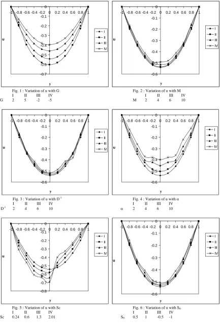
In this analysiswe discuss we effect of thermo diffusion and radiation on Non-Darcy convective heat and mass transfer flow of a viscous electrically conducting fluid through porous media in vertical channel in the presence of heat generating sources. The equation governing the flow heat and mass transfer or solved by employing a regular perturbation with δ as a perturbation Parameter.

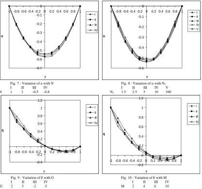
The axial velocity (u) is shown increases (1-8) for different values G, M, D-1, α, Sc, S0, N and N1 it is found that the

(6)

© 2014, IJMA. All Rights Reserved 64 (fig. 2 &3). From (fig.4), we find that |u| depreciates with increase heat generating sources. The variation of u with Schmidt number (Sc) shows that lesser molecular diffusivity larger |u| (fig.5). The flow region increase the Soret parameter |S0| leads to depreciation in |u| on the entire flow region (fig.6) with respect buoyancy force dominate thermal

buoyancy force. The magnitude of u enhances irrespective of the direction of the buoyancy forces (fig.7). From (fig.8) we find that higher the radiative heat flux smaller |u| in the flow region.

-0.7 -0.6 -0.5 -0.4 -0.3 -0.2 -0.1 0

-1 -0.8 -0.6 -0.4 -0.2 0 0.2 0.4 0.6 0.8 1

y u

I

II III

IV

-0.6 -0.5 -0.4 -0.3 -0.2 -0.1 0

-1 -0.8 -0.6 -0.4 -0.2 0 0.2 0.4 0.6 0.8 1

y u

I

II III

IV

Fig. 1 : Variation of u with G Fig. 2 : Variation of u with M

I II III IV I II III IV

G 2 5 -2 -5 M 2 4 6 10

-0.6 -0.5 -0.4 -0.3 -0.2 -0.1 0

-1 -0.8 -0.6 -0.4 -0.2 0 0.2 0.4 0.6 0.8 1

y u

I

II III

IV

-0.6 -0.5 -0.4 -0.3 -0.2 -0.1 0

-1 -0.8 -0.6 -0.4 -0.2 0 0.2 0.4 0.6 0.8 1

y u

I

II

III

IV

Fig. 3 : Variation of u with D-1 Fig. 4 : Variation of u with α

D-1 2 4 6 10 α 2 4 6 10

-0.8 -0.7 -0.6 -0.5 -0.4 -0.3 -0.2 -0.1 0

-1 -0.8 -0.6 -0.4 -0.2 0 0.2 0.4 0.6 0.8 1

y u

I

II III

IV

-0.6 -0.5 -0.4 -0.3 -0.2 -0.1 0

-1 -0.8 -0.6 -0.4 -0.2 0 0.2 0.4 0.6 0.8 1

y u

I

II III

IV

Fig. 5 : Variation of u with Sc Fig. 6 : Variation of u with S0

(7)

-0.7 -0.6 -0.5 -0.4 -0.3 -0.2 -0.1 0

-1 -0.8 -0.6 -0.4 -0.2 0 0.2 0.4 0.6 0.8 1

y

u

I

II

III

IV

-0.6 -0.5 -0.4 -0.3 -0.2 -0.1 0

-1 -0.8 -0.6 -0.4 -0.2 0 0.2 0.4 0.6 0.8 1

y

u

I II III IV V

Fig. 7 : Variation of u with N Fig. 8 : Variation of u with N1

I II III IV I II III IV V

N 1 2 -0.5 -0.8 N1 1.5 2.5 5 10 100

-0.4 -0.2 0 0.2 0.4 0.6 0.8 1 1.2

-1 -0.8 -0.6 -0.4 -0.2 0 0.2 0.4 0.6 0.8 1

y

q

I

II III

IV

-0.2 0 0.2 0.4 0.6 0.8 1 1.2

-1 -0.8 -0.6 -0.4 -0.2 0 0.2 0.4 0.6 0.8 1

y

q

I

II

III

IV

Fig. 9 : Variation of θ with G Fig. 10 : Variation of θ with M

G 2 5 -2 -5 M 2 4 6 10

The non–dimensional temperature (θ) is shown figures (9-16) for different parametric values. We follow the convention that non-dimensional temperature positive or negative according as the actual temperature is greater/lesser than T2. Fig.

9 represents θ with Grashof number G. It is found that the actual temperature reduces with increase with G>0 and

enhances with increase in G<0. The variation of θ with M and D-1 _{shows that the lesser permeability of porous}

medium/higher the Lorentz force, larger the actual temperature in the entire flow region (figs. 10 & 11). An increase in

the strength of heat generating source reduces the actual temperature in flow region .The variation of θ with Sc shows

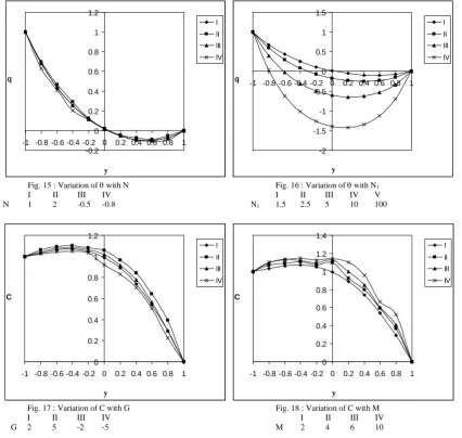
that the actual temperature reduces in the left half and enhances in the right half (fig.13). The variation of θ the Soret parameter S0 shows that an increase in |S0| enhances the actual temperature in the entire flow region (fig. 14).Then the

molecular buoyancy force dominates over the thermal buoyancy force, the actual temperature enhances when the buoyancy forces act in the same direction and for forces act in opposite direction it reduces in the flow region (fig. 15). From (fig. 16) we notice that higher the radiative heat flux smaller the actual temperature in the flow region.

-0.2 0 0.2 0.4 0.6 0.8 1 1.2

-1 -0.8 -0.6 -0.4 -0.2 0 0.2 0.4 0.6 0.8 1

y

q

I II III IV

-0.2 0 0.2 0.4 0.6 0.8 1 1.2

-1 -0.8 -0.6 -0.4 -0.2 0 0.2 0.4 0.6 0.8 1

y

q

I II III IV

Fig. 11 : Variation of θ with D-1 _{Fig. 12 : Variation of}_θ_with_α

(8)

-0.4 -0.2 0 0.2 0.4 0.6 0.8 1 1.2

-1 -0.8 -0.6 -0.4 -0.2 0 0.2 0.4 0.6 0.8 1

y

q

I

II

III

IV

-0.2 0 0.2 0.4 0.6 0.8 1 1.2

-1 -0.8 -0.6 -0.4 -0.2 0 0.2 0.4 0.6 0.8 1

y

q

I

II

III

IV

Fig. 13 : Variation of θ with Sc Fig. 14 : Variation of θ with S0

Sc 0.24 0.6 1.3 2.01 S0 0.5 1 -0.5 -1

The concentrate distribution (C) is shown in figs (17-24) for different parametric values. We follow the convention that the non-dimensional concentrate is positive or negative according as the actual concentration is greater/lesser than C2.

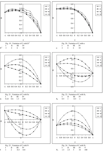
Fig.17 represents C with G. It is found that the actual concentration enhances with increase G>0 and for G<0 the actual concentration enhances in the left half and reduces right half of the channel. From (figs 18 & 19), we find that the actual concentration enhances with increase M and D-1 .The variation C with α shows that the actual concentration depreciates in the left half and enhances in the right half of the (fig. 20),the variation C with Sc shows that lesser the molecular diffusivity larger the actual concentration (fig. 21). The variation of C with Soret parameter S0 exhibits that

the actual concentration enhances with increase so>0 and depreciates with S0<0 (fig. 22). From fig.23, we find that the

actual concentration depreciates with N>0 and enhances with |N| (fig. 23). From (fig. 24) we notice that an increase in the radiation parameter N1 leads to an enhancement in the actual concentration (fig. 24).

-0.2 0 0.2 0.4 0.6 0.8 1 1.2

-1 -0.8 -0.6 -0.4 -0.2 0 0.2 0.4 0.6 0.8 1

y

q

I

II III

IV

-2 -1.5 -1 -0.5 0 0.5 1 1.5

-1 -0.8 -0.6 -0.4 -0.2 0 0.2 0.4 0.6 0.8 1

y

q

I

II III

IV

Fig. 15 : Variation of θ with N Fig. 16 : Variation of θ with N1

N 1 2 -0.5 -0.8 N1 1.5 2.5 5 10 100

0 0.2 0.4 0.6 0.8 1 1.2

-1 -0.8 -0.6 -0.4 -0.2 0 0.2 0.4 0.6 0.8 1

y

C

I

II III

IV

0 0.2 0.4 0.6 0.8 1 1.2 1.4

-1 -0.8 -0.6 -0.4 -0.2 0 0.2 0.4 0.6 0.8 1

y

C

I

II III

IV

Fig. 17 : Variation of C with G Fig. 18 : Variation of C with M

(9)

0 0.2 0.4 0.6 0.8 1 1.2 1.4

-1 -0.8 -0.6 -0.4 -0.2 0 0.2 0.4 0.6 0.8 1

y

C

I II III IV

0 0.2 0.4 0.6 0.8 1 1.2

-1 -0.8 -0.6 -0.4 -0.2 0 0.2 0.4 0.6 0.8 1

y

C

I II III IV

Fig. 19 : Variation of C with D-1 _{Fig. 20 : Variation of C with}_α

D-1 ₂ ₄ ₆ ₁₀ _α ₂ ₄ ₆ ₁₀

0 0.2 0.4 0.6 0.8 1 1.2 1.4 1.6

-1 -0.8 -0.6 -0.4 -0.2 0 0.2 0.4 0.6 0.8 1

y

C

I

II

III

IV

-1.5 -1 -0.5 0 0.5 1 1.5 2

-1 -0.8 -0.6 -0.4 -0.2 0 0.2 0.4 0.6 0.8 1

y

C

I

II

III

IV

Fig. 21 : Variation of C with Sc Fig. 22 : Variation of C with S0

Sc 0.24 0.6 1.3 2.01 S0 0.5 1 -0.5 -1

-2 -1.5 -1 -0.5 0 0.5 1 1.5

-1 -0.8 -0.6 -0.4 -0.2 0 0.2 0.4 0.6 0.8 1

y

C

I

II

III

IV

0 0.5 1 1.5 2 2.5 3

-1 -0.8 -0.6 -0.4 -0.2 0 0.2 0.4 0.6 0.8 1

y

C

I

II

III

IV

Fig. 23 : Variation of C with N Fig. 24 : Variation of C with N1

N 1 2 -0.5 -0.8 N1 1.5 2.5 5 10 100

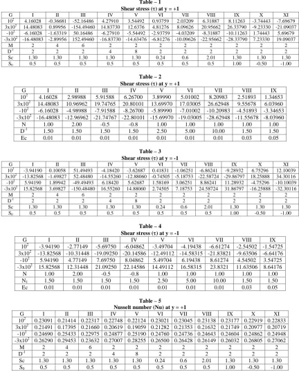
The rate of heat transfer (Nusselt number) at y=±1 is shown in (tables 1&4) for different parametric values. It is found that the rate of heat transfer depreciates with increase G>0 and enhance with G<0 at both the walls. An increase in M<4 reduces |Nu| for G>0 and enhance for G<0 and for higher for M>6. We notice a reversed effect in the behavior of |Nu|. The variation Nu with D-1 shows that lesser the permeability porous media smaller |Nu| in the heating case and the larger in the cooling case with respect to Sc. We find that lesser the molecular diffusivity larger |Nu| for G>0 and smaller for G<0 with respect to Soret parameter S0. We find that the rate of heat transfer enhance for G>0 and

depreciates with G<0 an increase S0>0 while for S0<0 a reversed effect observed in the behavior of |Nu| (tables 1&3) in

(10)

increase N1<2.5 depreciates |Nu| at y=+1 and enhance at y=-1 and for further higher N1>5 we notice an enhancement in

|Nu| for all G. The variation Nu with Eckert number Ec shows that higher the dissipative larger at y=+1 and smaller at y=-1 in the heating case and in the cooling case |Nu| reduces at y=±1 and enhance at y=-1 (tables 2&4).

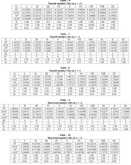
The rate of mass transfer (Sherwood number) at y=±1 we shown in tables (5-8) for different parametric values. We found that the rate of mass transfer enhance with |G|. An increase in Hartmann number M enhances |Sh| at the both the walls. With respect to D-1 we find that the rate of mass transfer depreciates with D-1≤4 and enhance with D-1>6 at y=±1 while at y=-1 |Sh| enhances for G>0 and depreciates for G<0. The variation of Sh with Sc shows that molecular diffusivity larger |sh| at y=+1 and y=-1 lesser |sh|. An increase Soret parameter S0 results an enhancement |Sh| at the

both walls (tables 5&7) when molecular buoyancy force dominates over the thermal buoyancy force the rate of mass transfer depreciates the both walls irrespective of. The direction of the buoyancy forces with respect to N1. We find that

higher radiative heat flux larger the rate of mass transfer at y=±1. An increase in Ec enhances |Sc| at y=+1 and depreciates at y=-1 (tables 6&8).

Table – 1 Shear stress (τ) at y = +1

G I II III IV V VI VII VIII IX X XI

102 4.16028 -0.36681 -52.16486 4.27910 3.54492 0.93759 2.03209 6.31887 8.11263 -3.74443 -7.69679 3x102 14.48083 0.89956 -154.49460 14.83730 12.6376 4.81276 8.09626 20.95662 26.33790 -9.23330 -21.09037

-102

-6.16028 -1.63319 50.16486 -6.27910 -5.54492 -2.93759 -4.03209 -8.31887 -10.11263 1.74443 5.69679 -3x102

-16.48083 -2.89956 152.49460 -16.83730 -14.63476 -6.81276 -10.09626 -22.95662 -28.33790 7.23330 19.09037

M 2 4 6 2 2 2 2 2 2 2 2

D-1

2 2 2 4 8 2 2 2 2 2 2

Sc 1.30 1.30 1.30 1.30 1.30 0.24 0.6 2.01 1.30 1.30 1.30

S0 0.5 0.5 0.5 0.5 0.5 0.5 0.5 0.5 1.00 -0.50 -1.00

Table – 2 Shear stress (τ) at y = +1

G I II III IV V VI VII VIII IX

102 4.16028 2.98988 5.91588 6.26700 3.89990 5.01002 8.20983 2.51893 1.34653 3x102 14.48083 10.96962 19.74765 20.80101 13.69970 17.03005 26.62948 9.55678 6.03960 -102 _-6.16028 _-4.98988 _-7.91588 _-8.26700 _-5.89990 _{-7.01002 -10.20983} _{-4.51893 -3.34653} -3x102 -16.48083 -12.96962 -21.74767 -22.80101 -15.69970 -19.03005 -28.62948 -11.55678 -8.03960

N 1.00 2.00 -0.5 -0.8 1.00 1.00 1.00 1.00 1.00

D-1 1.50 1.50 1.50 1.50 2.50 5.00 10.00 1.50 1.50

Ec 0.01 0.01 0.01 0.01 0.01 0.01 0.01 0.03 0.05

Table – 3 Shear stress (τ) at y = -1

102

-3.94190 0.10058 51.49493 -4.18420 -3.62687 0.41831 -1.06251 -6.86241 -9.28932 6.75296 12.10039 3x102

-13.82568 -1.69827 52.48480 -14.55260 -12.88060 -0.74505 -5.18753 -22.58724 -29.86797 18.25888 34.30116 -102 5.94190 1.89942 -49.49493 6.18420 5.62687 1.58169 3.06251 8.86241 11.28932 -4.75296 -10.10039 -3x102

15.82568 3.69827 -150.48480 16.55260 14.88060 2.74505 7.18753 24.58724 31.86797 -16.25888 -32.30116

M 2 4 6 2 2 2 2 2 2 2 2

D-1

2 2 2 4 8 2 2 2 2 2 2

Sc 1.30 1.30 1.30 1.30 1.30 0.24 0.6 2.01 1.30 1.30 1.30

S0 0.5 0.5 0.5 0.5 0.5 0.5 0.5 0.5 1.00 -0.50 -1.00

Table – 4 Shear stress (τ) at y = -1

102 -3.94190 -2.77149 -5.69750 -6.04862 -3.49704 -4.19438 -6.61274 -2.54502 -1.54725 3x102 -13.82568 -10.31448 -19.09250 -20.14586 -12.49112 -14.58315 -21.83821 -9.63506 -6.64176 -102 _5.94190 _4.77149 _7.69750 _8.04862 _5.49704 _6.19438 _8.61274 _4.54502 _3.54725 -3x102 15.82568 12.31448 21.09250 22.14586 14.49112 16.58315 23.8321 11.63506 8.64176

N 1.00 2.00 -0.5 -0.8 1.00 1.00 1.00 1.00 1.00

N1 1.50 1.50 1.50 1.50 2.50 5.00 10.00 1.50 1.50

Ec 0.01 0.01 0.01 0.01 0.01 0.01 0.01 0.03 0.05

Table – 5

Nusselt number (Nu) at y = +1

102 _{0.23091 0.21414 0.22317 0.22748 0.22124 0.23021 0.23045 0.23138 0.23177 0.22919 0.22833} 3x102 0.21491 0.17395 0.21660 0.20619 0.19059 0.21282 0.21353 0.21632 0.21749 0.20977 0.20719 -102 _{0.24690 0.25433 0.22975 0.24877 0.25190 0.24760 0.24736 0.24643 0.24604 0.24862 0.24948} -3x102 0.26290 0.29453 0.23632 0.27007 0.28255 0.26500 0.26428 0.26149 0.26032 0.26805 0.27062

M 2 4 6 2 2 2 2 2 2 2 2

D-1 ₂ ₂ ₂ ₄ ₈ ₂ ₂ ₂ ₂ ₂ ₂

Sc 1.30 1.30 1.30 1.30 1.30 0.24 0.6 2.01 1.30 1.30 1.30

(11)

Nusselt number (Nu) at y = +1

102 0.23091 0.23638 0.22271 0.22107 0.75039 1.93026 4.18476 0.14839 0.15719 3x102 0.21491 0.23132 1.19031 0.18539 0.73775 1.91878 4.17151 0.03866 0.11597 -102 0.24690 0.24143 0.25510 0.25674 0.76303 1.94174 4.19800 0.25813 0.19841 -3x102 0.26290 0.24649 0.28750 0.29242 0.77567 1.95322 4.21124 0.36786 0.23963

N 1.00 2.00 -0.5 -0.8 1.00 1.00 1.00 1.00 1.00

D-1 1.50 1.50 1.50 1.50 2.50 5.00 10.00 1.50 1.50

Ec 0.01 0.01 0.01 0.01 0.01 0.01 0.01 0.03 0.05

Table – 7 Nusselt number (Nu) at y = -1

102 -1.30765 -1.29298 -1.32520 -1.28687 -1.30536 -1.26765 -1.28765 -1.32705 -1.32765 -1.28760 -1.26765 3x102 _{-1.26765 -1.26298 -1.29526 -1.26667 -1.22531 -1.24760 -1.26762 -1.280765 -1.29765 -1.26785 -1.24760}

-102 -1.32705 -1.36298 -1.29520 -1.34682 -1.30561 -1.40760 -1.36785 -1.30705 -1.30705 -1.34765 -1.36765 -3x102 _{-1.36765 -1.39298 -1.34520 -1.38687 -1.40561 -1.46765 -1.38762 -1.34706 -1.38765 -1.36766 -1.38765}

M 2 4 6 2 2 2 2 2 2 2 2

D-1 2 2 2 4 8 2 2 2 2 2 2

Sc 1.30 1.30 1.30 1.30 1.30 0.24 0.6 2.01 1.30 1.30 1.30

S0 0.5 0.5 0.5 0.5 0.5 0.5 0.5 0.5 1.00 -0.50 -1.00

Table –8

Nusselt number (Nu) at y = -1

102 -1.30765 -1.32765 -1.30765 -1.28765 -1.69712 -2.75578 -4.94078 -1.27200 -1.24654 3x102 -1.28765 -1.29765 -1.29765 -1.27760 -1.66712 -2.72578 -4.90078 -1.26206 -1.22654 -102 -1.32760 -1.34765 -1.34765 -1.36766 -1.70712 -2.78578 -4.99078 -1.29202 -1.34650 -3x102 -1.34762 -1.32765 -1.36765 -1.308795 -1.72712 -2.82578 -4.52078 -1.32201 -1.36656

N 1.00 2.00 -0.5 -0.8 1.00 1.00 1.00 1.00 1.00

N1 1.50 1.50 1.50 1.50 2.50 5.00 10.00 1.50 1.50

Ec 0.01 0.01 0.01 0.01 0.01 0.01 0.01 0.03 0.05

Table – 9

Sherwood number (Sh) at y = +1

102 -1.06061 -3.76430 -23.01955 -1.01422 -2.15113 -0.30533 -0.55992 -1.57607 -2.01025 0.76147 1.63390 3x102 -2.56596 -4.54511 -24.25677 -1.31654 -2.54010 0.23843 -0.42900 -3.13346 3.62257 1.31562 2.14060 -102 -1.55525 -2.98348 -21.78232 -1.51230 -1.76217 -0.84909 -1.09084 -2.01867 -2.39793 0.20732 1.12721 -3x102 -2.04989 -2.20266 -20.54510 -1.61018 -1.87320 -1.39285 -1.62175 -2.46127 -2.78561 -0.34682 0.62052

M 2 4 6 2 2 2 2 2 2 2 2

D-1 2 2 2 4 8 2 2 2 2 2 2

Sc 1.30 1.30 1.30 1.30 1.30 0.24 0.6 2.01 1.30 1.30 1.30

S0 0.5 0.5 0.5 0.5 0.5 0.5 0.5 0.5 1.00 -0.50 -1.00

Table – 10

Sherwood number (Sh) at y = +1

102 -1.06061 -0.41016 3.36666 2.30701 1.74014 2.26479 10.24214 -1.08032 -1.15836 3x102 -2.56596 -0.04246 4.14881 3.1162 1.25255 9.14617 39.55516 -0.68320 -0.95881 -102 _{-1.55525 -0.77786 2.58452 1.50241 -2.73283} _{-6.61660 -19.07089 -1.64829 -1.95792}

-3x102 _{-2.04989 -1.14555 1.80237 0.69780 -4.72552 -14.49798 -48.38392 -2.13732 -2.55747}

N 1.00 2.00 -0.5 -0.8 1.00 1.00 1.00 1.00 1.00

D-1 _1.50 _1.50 _1.50 _1.50 _2.50 _5.00 _10.00 _1.50 _1.50

Ec 0.01 0.01 0.01 0.01 0.01 0.01 0.01 0.03 0.05

6. REFERENCES

1. Abdul Sattar, Md. And Alam,Md : Thermal diffusion as well as transprotaion effect on MHD free convection and Mass Transfer flow past an accelerated vertical porous plate, Ind Journal of Pure and Applied Maths. Vol. 24, pp.679-688(199

2. Ayani,M.B. and Fsfahani,J.H.: The effect of radiation on the natural convection induced by a line heat source.Int.J.Nummer.Method,Heat fluid flow (U.K.),16,28-45(2006)

3. Balasubramanyam M, Sudarsan Reddy P, Prasada Rao D.R.V.: Non-Darcy viscous electrically conducting heat and mass transfer flow through a porous medium in a vertical channel in the presence on heat generating sources, Int. J. of Appl. Math and Mech. Vol.6 (15), pp.45-45, (2010).

4. Beckermann C.. Visakanta R.and Ramadhyani S.: A numerical study of non-Darcian natural convection in a vertical enclosure filled with a porous medium., Numerical Heat transfer 10, pp.557-570

(12)

embedded in a non-Darcian porous medium in the presence of a homogeneous chemical reaction, Nonlinear Analysis: Modeling and control, vol.15, No.2, pp.139-154 (2010).

7. P.Cheng : Heat transfer in geothermal systems., Adv. Heat transfer 14,1-105(1978).

8. Devika Rani B, Vijaya Bhaskar Reddy P, Prasada Rao D.R.V. : Effect of radiation on Non-Darcy convective Heat Transfer through a Porous medium in a vertical channel, J. Comp. & Mech. Sci. Vol.2(3), pp.483-492 (2011).

9. Jha, B. K. and Singh, A. K.: ,Astrophys. Space Sci. vol.173, p.251 (1990). 10. Kafousia.N.G. ,Astrophys. Space Sci. vol.173, p.251(1990)

11. Kalidas.N. and Prasad, V: Benard convection in porous media Effects of Darcy and Pransdtl Numbers, Int. Syms. Convection in porous media, non-Darcy effects, proc.25th Nat. Heat Transfer Conf.V.1, pp.593-604 (1988)

12. Kumar. A., Singh,N.P., Singh,A.K.., Kumar,H.: MHD free convection flow of a viscous fluid past a porous vertical plate through non-homogeneous porous medium with radiation and temperature gradient dependent heat source in slip glow regime, Ultra Sci.Phys.Sci (India) ,18,39-46(2006)

13. Malasetty.M.S,Gaikwad.S.N: Effect of cross diffusion on double diffusive convection in the presence of horizontal gradient,Int.Journal Eng.Science, Vol.40,PP773-787(2002)

14. Poulikakos D., and Bejan, A.: The Departure from Darcy flow in Nat. Convection in a vertical porous layer, physics fluids V.28,pp.3477-3484 (1985)

15. Prasad, V.and Tuntomo, A.: Inertia Effects on Natural Convection in a vertical porous cavity, numerical Heat Transfer, V.11, pp.295-320 (1987)

16. Prasad.V: Natual convectin inporous media.,Ph.D theisi,S.K.University, Anantapur (1983)

17. Prasad.V, F.A, Kulacki and M.keyhani;” Natural convection in a porous medium” J.Fluid Mech.150p.89-119(`1985).

18. Rashad A.M., Bakier A.Y.: MHD effects on non-Darcy forced convection boundary layer flow past a permeable wedge in a porous medium with uniform heat flux, Nonlinear Analysis: Modeling and control, vol.14, No.2, pp.249-261 (2009).

19 D. Tien, C.V. and Hong, J.T.: Natural convection in porous media under non-Darcian and non-uniform permeability conditions, hemisphere, Washington.C. (1985)

20. T.L.Tong and E.Subramanian: A boundary layer analysis for natural correction in porous enclosures: use of the Brinkman-extended Darcy model,., Int.J.Heat Mass Transfer.28,pp.563-571.

21. Vafai, K., Tien, C.L: Boundary and Inertia effects on flow and Heat Transfer in Porous Media, Int. J. Heat Mass Transfer, V.24. Pp.195-203 (1981)

22. Vafai, K., Thyagaraju, R.: Analysis of flow and heat Transfer at the interface region of a porous medium, Int. J. Heat Mass Trans., V.30pp.1391-1405 (1987)

23. G.Laurait and V.Prasad.: natural convection in a vertical porous cavity a numerical study of Brinkman extended Darcy formulation., J. Heat Transfer.pp.295-320(1987).