Available online throug
ISSN 2229 – 5046
International Journal of Mathematical Archive- 6(8), August – 2015 216
SOLUTION OF SECOND KIND VOLTERRA INTEGRAL AND INTEGRO-DIFFERENTIAL
EQUATION BY BERNSTEIN POLYNOMIALS METHOD
MOHAMMED. KHALID SHAHOOTH
*, OMAR. K. AL-HUSSEINI**
Pure Mathematics, Department of Mathematics,
Faculty Science and Technology, National University of Malaysia.
(Received On: 27-06-15; Revised & Accepted On: 27-07-15)
ABSTRACT
I
n this paper, we introduce a solution of second kind Volterra integral and integro-differential equations by using Bernstein polynomials method (BPM). First, we introduce the proposed method, then we used it to transform the integral and integro-differential equations to the system of algebraic equations. Finally, the numerical examples illustrate the efficiency and accuracy of this method.Keywords: Integral Equations, Integro-differential Equations, Bernstein polynomials method.
1. INTRODUCTION
Volterra integral equation arise in engineering, physics, chemistry and biological problems such as parabolic boundary value problems, the spatio-temporal development of the epidemic, population dynamics and semi-conductor device. Many initial and boundary value problems associated with the ordinary and partial differential equations can be cast into the Volterra integral equation types. The Volterra integral equation was first used by Vito Volterra [1] in 1884.
Mathematical modelling of real-life problems usually results in functional equations, e.g. partial differential equations, integral and integro-differential equations, stochastic equations and others. Many mathematical formulation of physical phenomena contain integro-differential equations, these equations arises in fluid dynamics, biological models and chemical kinetics [2], for more details see [3,4]. This type of equations was introduced by Volterra for the first time in the early 1900. Volterra investigated the population growth, focussing his study on the hereditary influences, where through his research work the topic of integro-differential equations was established [5].
There are several numerical and analytical methods have been used to solve Volterra integral equations. For Example, A new approach to solve Volterra integral equation by using Bernstein's approximation is employed in [6]. Application of Collocation method on Volterra integral equations are investigated in [7, 8]. Taylor series expansion method is used for second kind Volterra integral equation in [9]. In [10] Chebyshev polynomials is used to find numerical solution of nonlinear Volterra integral equations of the second kind.[11] applied Variational iteration method to solve integral equation. Application of Adomian’s decomposition method to solve integral equations are found in [12, 13]. Numerical solution of the second kind Volterra integral equation using an expansion method is employed in [14].
Integro-differential equations are usually difficult to solve analytically so it is required to obtain an efficient approximate solution. So, they have been of great interest by several authors. In literature, there exist many numerical and semi-analytical-numerical techniques to solve Integro-differential equation. For Example, Application of Adomian's decomposition method on Integro-differential equation are investigated in [15, 12, 13]. Comparison between Wavelet Galerkin method and Adomian's decomposition method to solve integro differential equation is found in [16]. The Tau method is applied to the integro-differential equation in [17]. [18] used Taylor polynomials to solve high-order Volterra integro-differential equation. Wavelet Galerkin method (WGM) to solve integro-differential equation can be found in [19]. In [20] Collocation method is used to solve fractional integro-differential equation. Application of He's Homotopy perturbation method to solve Volterra integro-differential equation are found in [21, 22]. Solution of forth-order integro - differential equation using variational iteration method can be found in [2]. In [23] rationalized Haar functions method is applied on system of linear integro-differential equations. In [24, 25] integro-differential equation is studied by using the differential transform method.
Corresponding Author: Mohammed. Khalid. Shahooth
*, Pure Mathematics,
Bernstein polynomials method (BPM) has been recently used for the solution of integral and integro-differential equations. For example, Bernstein polynomials is applied to find an approximate solution for Fredholm integro-Differential equation and integral equation of the second kind in [26].[27] investigated the application of Bernstein polynomials for deriving the modified Simpson's 3/8, and the composite modified Simpson's 3/8 to solve one dimensional linear Volterra integral equations of the second kind. This method is employed to find an approximate solution of Fredholm integral equation of the second kind in [28].
In this paper, we propose Bernstein polynomials method to solve second kind Volterra integral and integro-differential equations. We have introduced that the BPM is very powerful and efficient technique in finding analytical solutions for the second kind Volterra integral and integro-differential equations.
A second kind Volterra integral and integro-differential equations are represented respectively in the form:
( )
( )
0
( , ) ( ) ,
x
u x
=
f x
+
λ
∫
k x t u t dt
(1)( )
( )
( )
0
( , ) ( ) ,
x n
u
x
=
f x
+
λ
∫
k x t u t dt
(2)Where
a
≤ ≤
x
b
,
are scalar parameters and is the continuous function,k x t
( , )
is the kernel of integralequation, ( )
( )
n n
n
d u
u
x
dx
=
and is the unknown function to be determine.2. BERNSTEIN POLYNOMIALS METHOD (BPM)
Polynomials are incredibly useful mathematical tools as they are simply defined, can be calculated quickly on computer systems and represent a tremendous variety of functions. The Bernstein polynomials of degree - n are defined by [29]:
B t
in( )
n
t
i(1
t
)
n ii
−
=
−
fori
=
0,1, 2,...,
n
(3)Where
(
!
)
!
!
n
n
i
i n i
=
−
, (n) is the degree of polynomials, (i) is the index of polynomials and (t) is the variable.The exponents on the (t) term increase by one as (i) increases, and the exponents on the (1-t) term decrease by one as (i) increases. The Bernstein polynomials of degree - n can be defined by blending together two Bernstein polynomials of degree (n-1) That is, the -degree Bernstein polynomial can be written as [29]:
1 1
1
( )
(1
)
( )
( )
n n n
k k k
B t
= −
t B
−t
+
tB
−−t
(4)Bernstein polynomials of degree (n) can be written in terms of the power basis. This can be directly calculated using the equation (3) and the binomial theorem as follows [26]:
( )
(1
)
( 1)
n
n k n k i k i
k
i k
n
n
i
B t
t
t
t
k
i
k
− −
=
=
−
=
−
∑
(5)Where the binomial theorem is used to Expand
(1
−
t
)
n k− . The derivatives of the -degree Bernstein polynomials are polynomials of degree (n-1)(
1 1)
1( )
(1
)
( )
( ) , 0
.
n k n k n n
k k k
n
d
d
B t
t
t
n B
t
B
t
k
n
k
dt
dt
− − −
−
=
−
=
−
≤ ≤
(6)3. A MATRIX REPRESENTATION FOR BERNSTEIN POLYNOMIALS
In many applications, a matrix formulation for the Bernstein polynomials is useful. These are straight forward to develop if only looking at a linear combination in terms of dot products. Given a polynomial written as a linear combination of the Bernstein basis functions [26]:
0 0 1 1 2 2
( )
n( )
n( )
n( )
n nn( )
© 2015, IJMA. All Rights Reserved 218 It is easy to write this as a dot product of two vectors
0 1
0 1 2 2
( )
n( )
n( )
n( ) . . .
nn
( )
n
c
c
B t
B t
B t
B t
B t
c
c
=
(8)which can be converted to the following form:
00 0
10 11 1
2
20 21 22 2
0 1 2
0
0
0
0
0
( )
1 ...
n0
n n n nn n
b
c
b
b
c
B t
t t
t
b
b
b
c
b
b
b
b
c
=
(9)where are the coefficients of the power basis that are used to determine the respective Bernstein polynomials, we note that the matrix in this case lower triangular. The matrix of derivatives of Bernstein polynomials is: [26].
00 0
10 11 1
1
20 21 22 2
0 1 2
0
0
0
0
0
( )
0 1 2 ...
n0
n n n nn n
b
c
b
b
c
B t
t
nt
b
b
b
c
b
b
b
b
c
−
′
=
(9a)4. SOLUTION FOR VOLTERRA INTEGRAL EQUATIONS OF THE SECOND KIND
In this section Bernstein polynomials method is proposed to find an approximate solution for Volterra integral equations of the second kind. Consider the Volterra integral equation of the second kind in equation (1).
Applying the following equation:
0 1
0 1 2 2
( )
n( )
n( )
n( )
nn
( )
n
c
c
u x
B x B x B x
B x
c
c
=
(10)Substituting (10) into equation (1) we get:
0
1 0
( )
1( )
2( )
( )
2n n n n
n
n
c
c
B x B x B x
B x
c
c
0 10 1 2 2
( )
( , )
( )
( )
( )
( )
x
n n n n
n a
n
c
c
f x
k x t
B
t
B
t
B
t
B
t
c
c
λ
=
+
∫
Using the following equation into equation (11) we have:
0 1 2
0 1 2 2
( )
1
n n
( )
n( )
n( )
nn
( )
n
c
c
u t
x x
x
B x
B x
B x
B x
c
c
=
(12) 0 1 0( ) ( ) ( )
1 2( )
2n n n n
n
n
c
c
B x B x B x
B x
c
c
00 010 11 1
2
20 21 22 2
0 1 2
0
0
0
0
0
( )
( , ) 1
0
x
n
a
n n n nn n
b
c
b
b
c
f x
k x t
t t
t
b
b
b
c
dt
b
b
b
b
c
λ
=
+
∫
(13)Now to find the Volterra integration in equation (13). Then in order to determine
c c
0, ,... .
1c
n we need n equations. Now choicex i
i,
=
1, 2, 3...,
n
in the interval[ ]
a b
,
, which gives n equations. Solve the n equations by Gauss elimination to find the values ofc c
0, ,... .
1c
n5. SOLUTION FOR VOLTERRA INTEGRO-DIFFERENTIAL EQUATIONS OF THE SECOND KIND
In this section Bernstein polynomials method is used to find the approximate solution for Volterra integro - differential equation of the second kind. Consider the Volterra integro-differential equation of the second kind in equation (2).
0 1 ( )
0 1 2 2
( )
( )
( )
( )
( )
n n n n n
n
n
c
c
u
x
B x B x B x
B x
c
c
=
(14)Substituting (14) into equation (2), we get:
0 1 0
( ) ( ) ( )
1 2( )
2n
n n n n
n
n
c
c
B x B x B x
B x
c
c
0 10 1 2 2
( )
( , )
( ) ( ) ( )
( )
x
n n n n
n a
n
c
c
f x
k x t
B t B t B t
B t
c
c
λ
=
+
∫
© 2015, IJMA. All Rights Reserved 220 Using the following equation into equation (15) we have:
0 1 2
0 1 2 2
( )
1
n n
( )
n( )
n( )
nn
( )
n
c
c
u t
x x
x
B x
B x
B x
B x
c
c
=
(16) 0 10
( ) ( ) ( )
1 2( )
2n
n n n n
n
n
c
c
B
x B
x B
x
B
x
c
c
00 010 11 1
2
20 21 22 2
0 1 2
0
0
0
0
0
( )
( , ) 1
0
x
n
a
n n n nn n
b
c
b
b
c
f x
k x t
tt
t
b
b
b
c
dt
b
b
b
b
c
λ
=
+
∫
(17)Now to find all differentiation here, and the Volterra integration in equation (17). Then in order to determine
0
, ,... .
1 nc c
c
we need n equations. Now choicex i
i,
=
1, 2, 3...,
n
in the interval[ ]
a b
,
, which gives n equations. Solve the n equations by Gauss elimination to find the values ofc c
0, ,... .
1c
n . The following algorithm summarizes the steps for finding the solution for the second kind Volterra integral and integro-differential equations of the second kind. .6. ALGORITHM (BPM)
Input:
(
f x k x t u x a b
( ), ( , ), ( ), , ,
λ
)
Output: polynomials of degree n
Step-1: Choice n the degree of Bernstein polynomials
( )
(1
)
n i n i
i
n
B t
t
t
i
−
=
−
fori
=
0,1, 2,...,
n
Step-2: Put the Bernstein polynomials in the linear Volterra integral and integro-differential equations of the second kind
00 0
10 11 1
( ) 1
20 21 22 2
0 1 2
0
0
0
0
0
( )
0 1 2
0
n n
n n n nn n
b
c
b
b
c
u
x
t
nt
b
b
b
c
b
b
b
b
c
−
=
0 10 1 2 2
( )
( , )
( ) ( ) ( )
( )
x
n n n n
n a
n
c
c
f x
k x t
B
t B
t B
t
B
t
c
( )
( )
( , )
( )
x
n n
i i
a
B x
=
f x
+
∫
k x t B t dt
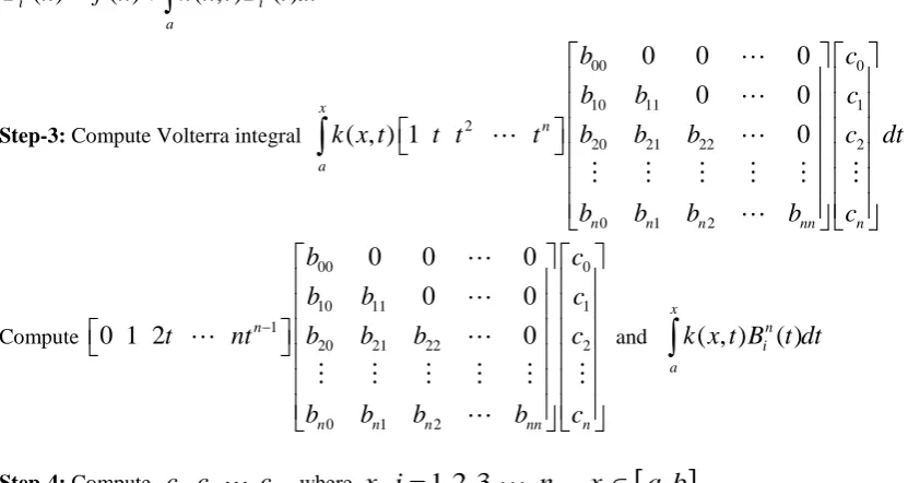
Step-3: Compute Volterra integral
00 0
10 11 1
2
20 21 22 2
0 1 2
0
0
0
0
0
( , ) 1
0
x
n
a
n n n nn n
b
c
b
b
c
k x t
t t
t
b
b
b
c
dt
b
b
b
b
c
∫
Compute
00 0
10 11 1
1
20 21 22 2
0 1 2
0
0
0
0
0
0 1 2
n
0
n n n nn n
b
c
b
b
c
t
nt
b
b
b
c
b
b
b
b
c
−
and
( , )
( )
x
n i a
k x t B t dt
∫
Step-4: Compute
c c
0, ,
1
,
c
n , wherex i
i,
=
1, 2, 3,
, ,
n
x
i∈
[ ]
a b
,
End.
7. NUMERICAL EXPERIMENTS
In this section we apply BPM to solving the linear Volterra integral and integro-differential equations of the second kind. Also we presented here two linear Volterra integral equations and two linear Volterra Integro-differential equations. These four examples, the first two examples are solved by Adomian’s decomposition method (ADM) [13]. And the last two examples are solved by Homotopy analysis method (HAM) [5].The computations associated with these examples were performed using Matlab ver.2013a.
Example1: Consider the following Volterra integral equation of the second kind [13].
( )
1
0x( )
u x
= −
∫
u t dt
, with the exact solutionu x
( )
=
e
−x.
Here we can noticed that
f x
( )
=
1 ,
λ
= −
1
andk x t
( , )
=
1.
Table (1): Numerical results for example 1 with exact solution
0 1.0000 1.0000 1.0000 1.0000
© 2015, IJMA. All Rights Reserved 222
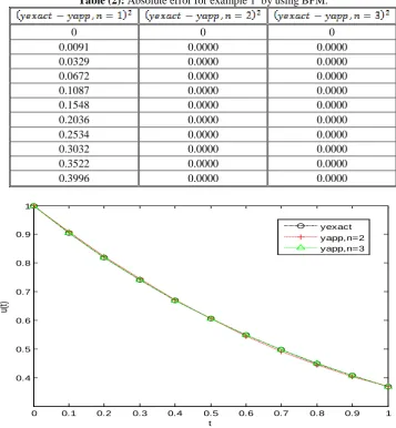
Table (2): Absolute error for example 1 by using BPM.
0 0 0
0.0091 0.0000 0.0000
0.0329 0.0000 0.0000
0.0672 0.0000 0.0000
0.1087 0.0000 0.0000
0.1548 0.0000 0.0000
0.2036 0.0000 0.0000
0.2534 0.0000 0.0000
0.3032 0.0000 0.0000
0.3522 0.0000 0.0000
0.3996 0.0000 0.0000
0 0.1 0.2 0.3 0.4 0.5 0.6 0.7 0.8 0.9 1
0.4 0.5 0.6 0.7 0.8 0.9 1
t
u(t
)
yexact yapp,n=2 yapp,n=3
Figure-1: 3rd-order approximate solution by BPM and exact solution.
Example 2: Consider the following Volterra integral equation of the second kind [13].
0
( )
1
(
) ( )
x
u x
= +
∫
t
−
x u t dt
, with the exact solutionu x
( )
=
cos( ).
x
Also we can noticed that
f x
( )
=
1,
λ
=
1
andk x t
( , )
= −
(
t
x
).
Table (1): Numerical results for Example 2 with exact solution
0 1.0000 1.0000 1.0000 1.0000
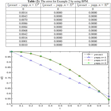
Table (2): The error for Example 2 by using BPM.
0 0 0
0.0014 0.0000 0.0000
0.0043 0.0000 0.0000
0.0070 0.0000 0.0000
0.0086 0.0000 0.0000
0.0084 0.0000 0.0000
0.0068 0.0000 0.0000
0.0042 0.0000 0.0000
0.0016 0.0000 0.0000
0.0001 0.0000 0.0000
0.0010 0.0000 0.0000
0 0.1 0.2 0.3 0.4 0.5 0.6 0.7 0.8 0.9 1
0.5 0.55 0.6 0.65 0.7 0.75 0.8 0.85 0.9 0.95 1
t
u(t
)
yexact yapp,n=1 yapp,n=2 yapp,n=3
Figure-2: 3rd-order approximate solution by BPM and exact solution.
Example 3: Consider the following Volterra integro-differential equation of the second kind [5].
0
( ) 1
( ) , (0)
0
x
u x
′
= −
∫
u t dt u
=
, and the exact solution isu x
( )
=
sin( ).
x
Table (1): Numerical results for Example 3 with exact solution
yexact
yapp n
,
=
1
yapp n
,
=
2
yapp n
,
=
3
0 0 0 0 0
0.1000 0.0998 0.0667 0.1180 0.1009
0.2000 0.1987 0.1333 0.2290 0.2002
0.3000 0.2955 0.2000 0.3329 0.2970
0.4000 0.3894 0.2667 0.4298 0.3906
0.5000 0.4794 0.3333 0.5196 0.4803
0.6000 0.5646 0.4000 0.6023 0.5652
0.7000 0.6442 0.4667 0.6780 0.6445
0.8000 0.7174 0.5333 0.7466 0.7176
0.9000 0.7833 0.6000 0.8082 0.7836
© 2015, IJMA. All Rights Reserved 224
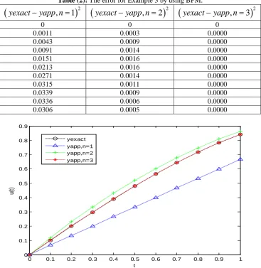
Table (2): The error for Example 3 by using BPM.
(
)
2,
1
yexact
−
yapp n
=
(
yexact
−
yapp n
,
=
2
)
2(
yexact
−
yapp n
,
=
3
)
20 0 0
0.0011 0.0003 0.0000
0.0043 0.0009 0.0000
0.0091 0.0014 0.0000
0.0151 0.0016 0.0000
0.0213 0.0016 0.0000
0.0271 0.0014 0.0000
0.0315 0.0011 0.0000
0.0339 0.0009 0.0000
0.0336 0.0006 0.0000
0.0306 0.0005 0.0000
0 0.1 0.2 0.3 0.4 0.5 0.6 0.7 0.8 0.9 1
0 0.1 0.2 0.3 0.4 0.5 0.6 0.7 0.8 0.9
t
u(t
)
yexact yapp,n=1 yapp,n=2 yapp,n=3
Figure-3: 3rd-order approximate solution by BPM and exact solution.
Example 4: Consider the following Volterra integro-differential equation of the second kind [5].
0
( )
1
(
) ( )
,
(0
)1 ,
(0
)1
x
u
′′
x
= + +
x
∫
x
−
t u t dt
u
=
u
′
=
and the exact solution isu x
( )
=
e
x.
Table (1): Numerical results for Example 4 with exact solution
0 1.0000 1.0000 1.0000 1.0000
Table (2): The error for Example 4 by using BPM.
(
)
2,
1
yexact
−
yapp n
=
(
yexact
−
yapp n
,
=
2
)
2(
yexact
−
yapp n
,
=
3
)
20 0 0
0.0000 0.0000 0.0000
0.0005 0.0001 0.0000
0.0025 0.0006 0.0000
0.0084 0.0016 0.0000
0.0221 0.0033 0.0001
0.0493 0.0056 0.0004
0.0984 0.0082 0.0009
0.1811 0.0105 0.0017
0.3132 0.0118 0.0030
0.5159 0.0114 0.0047
0 0.1 0.2 0.3 0.4 0.5 0.6 0.7 0.8 0.9 1
1 1.2 1.4 1.6 1.8 2 2.2 2.4 2.6 2.8 3
t
u(t
)
yexact yapp,n=1 yapp,n=2 yapp,n=3
Figure-4: 3rd-order approximate solution by BPM and exact solution.
CONCLUSION
In this paper, we have successfully used BPM for solving Volterra integral and integro-differential equations of the second kind.The integral equations are usually difficult to solve analytically. In many cases, it is required to obtain the numerical solution, for this purpose the presented method can be proposed and it’s apparently seen that BPM is a powerful and easy-to-use analytic tool for finding the solutions for integral and integro-differential equations. Numerical experiments in comparison with other methods such as Adomian's decomposition method (ADM) and Homotopy analysis method (HAM).The results shown the efficiency of the Bernstein polynomials method (BPM) for solving this type of equations. Also we noted that when the degree of Bernstein polynomials is increasing the errors decrease to smaller values.
REFERENCES
1. V. Volterra, Theory of functional of integral and integro-differential equations, Dover, New York, (1959). 2. N. Sweilam, Fourth order integro-differential equations using variational iteration method, Compu. Math.
Appl., 54 (2007), 1086-1091.
3. P.K. Kythe, P. Puri, Computational methods for linear integral equations, University of New Orlans, New Orlans, 2002.
4. A.M. Wazwaz, A comparison study between the modified decomposition method and the traditional methods for solving nonlinear integral equations, Applied Mathematics and Computation (in press).
5. K. Shah, T. Singh, Solution of second kind Volterra integral and integro-differential equation by Homotopy analysis method,International Journal of Mathematical Archive,6(2015), 49-59.
6. K. Maleknejad, E. Hashemizadeh, R. Ezzati, A new approach to the numerical solution of Volterra integral equations by using Bernstein's approximation, Commu. Nonlinear Sci. Num. Simul., 16 (2011), 647-655. 7. H. Brunner, On the Numerical Solution of Nonlinear Volterra-Fredholm Integral Equations by Collocation
Methods, SIAM Jour. Numer. Anal., 27 (1990), 987-1000.
© 2015, IJMA. All Rights Reserved 226 9. K. Maleknejad, N. Agazadeh, Numerical solution of Volterra integral equations of the second kind with
convolution kernel by using Taylor-series expansion method, Appl. Math. Compu., 161 (2005), 915-922. 10. K. Maleknejad, S. Sohrabi, Y. Rostami, Numerical solution of nonlinear Volterra integral equations of the
second kind by using Chebyshev polynomials, Appl. Math. Compu., 188 (2007), 123-128. 17.
11. L. Xu, Variational iteration method for solving integral equations, I. Jour. comp. math. appl., 54 (2007), 1071-1078.
12. A. Wazwaz, Two methods for solving integral equations, Appl. Math. Compu., 77 (1996), 79-89.
13. A. Wazwaz, Linear and Nonlinear Integral Equations: Methods and Applications, Higher education press, Springer, (2011).
14. M. Rabbani, K. Maleknejad, N. Aghazadeh, Numerical computational solution of the Volterra integral equations system of the second kind by using an expansion method, Appl. Math. Compu., 187 (2007), 1143-1146.
15. I. Hashim, Adomian decomposition method for solving BVPs for fourth-order integro- differential equations, Jour. Compu. Appl. Math., 193 (2006), 658-664.
16. S. El-Sayed, M. Abdel-Aziz, A comparison of Adomian's decomposition method and Wavelet-Galerkin method for integro-differential equations, Appl. Math. Compu., 136 (2003), 151-159.
17. S. Hosseini, S. Shahmorad, Numerical solution of a class of Integro-Differential equations by the Tau Method with an error estimation, Appl. Math. Compu., 136 (2003), 559-570.
18. K. Maleknejad, Y. Mahmoudi, Taylor polynomial solution of high-order nonlinear Volterra-Fredholm integro differential equations, Appl. Math. Compu., 145 (2003), 641-653.
19. A. Avudainayagam, C. Vani, Wavelet-Galerkin method for integro-differential equations, Appl. Numer. Math., 32 (2000), 247-254.
20. E. Rawashdeh, Numerical solution of fractional integro-differential equation by collocation method, Appl. Math. Compu., 176 (2006), 1-6.
21. M. Dehghan, F. Shakeri, Solution of an integro-differential equation arising in oscillating magnetic field using He's Homotopy Perturbation method, PIER, 78 (2008), 361-376.
22. M. El-Shahed, Application of He's Homotopy Perturbation Method to Volterra Integro-differential equation, Int. Jour. Nonlinear Sci. Num. Simulat., 6 (2005), 163-168. 16.
23. K. Maleknejad, F. Mirzaee, S. Abbasbandy, Solving linear integro-differential equations system by using rationalized Haar function method, Appl. Math. Compu., 155 (2005), 317- 328.
24. A. Arikoglu, I. Ozkol, Solution of boundary value problems for integro-differential equations by using differential transform method, Appl. Math. Compu., 168 (2005), 1145-1158.
25. P. Darnaia, A. Ebadian, A method for the numerical solution of the integro-differential equations, Appl. Math. Compu., 188 (2007), 657-668.
26. A. AL-Juburee, Approximate Solution for linear Fredholm Integro-Differential Equation and Integral Equation by Using Bernstein Polynomials method, Journal of the Faculty of Education .Al- Mustansiriyah University. Iraq, (2010).
27. J. Ahmad, Deriving the Composite Simpson Rule by Using Bernstein Polynomials for Solving Volterra Integral Equations. Baghdad Science Journal, 11(2014).
28. H. Ali, S. Hussain, The Collocation Method for Solving the Linear Fredholm Integral Equation of the Second Kind Using Bernstein Polynomials, Eng. Tech. Journal, 28(2010).
29. K.Joy, Bernstein Polynomials, On-Line Geometric Modeling Notes, 2000.
Source of support: Nil, Conflict of interest: None Declared