http://www.sciencepublishinggroup.com/j/ajomis doi: 10.11648/j.ajomis.20190401.11
ISSN: 2578-8302 (Print); ISSN: 2578-8310 (Online)
The Value of Inventory Accuracy in Supply Chain
Management: Correlation Between Error Sources and
Proactive Error Correction
Assaf Avrahami, Evgeni Korchatov
Faculty of Industrial Engineering, Israel Institute of Technology, Haifa, Israel
Email address:
To cite this article:
Assaf Avrahami, Evgeni Korchatov. The Value of Inventory Accuracy in Supply Chain Management: Correlation Between Error Sources and Proactive Error Correction. American Journal of Operations Management and Information Systems. Vol. 4, No. 1, 2019, pp. 1-15.
doi: 10.11648/j.ajomis.20190401.11
Received: December 18, 2018; Accepted: February 13, 2019; Published: March 1, 2019
Abstract:
One of the key elements in supplay cahin management is accurate information. Decision makers are aware of inaccuracies in inventory levels and, therefore, routinely conduct inventory reviews to correct the discrepancies between IT records and actual inventory. Several studies have investigated error sources and the cumulative effect of errors on holding costs, shortage costs, order-up-to levels and time between inventory counts. In most works, the errors were independent of the demand, which is neither realistic nor accurate. Here we use familiar inventory errors and information scenarios already proposed in several previous papers. We offer a model that considers the correlation between inventory errors and demand. The effect of the relationship between the random variables is tested in the context of several different scenarios. Each scenario contains a different level of information about the underlying demand and inventory errors. We then analyze the effect of changes of the covariance on the cost and time between inventory counts in each scenario. Using these results we formulate the value of information and its dependence on the covariance. We use analytical methods to draw conclusions regarding single parameter set cases and a numerical full factorial study for average multiparameter cases. In both settings, we show that the value of information decreases as the covariance increases. Moreover, the reduction is more significant when the information scenario makes less assumptions. The same behavior is observed in stock review frequency. As covariance increases, the optimal number of periods between inventory reviews drops sharply. Finally, we propose several simple methods for proactive error correction. We show that without prior knowledge, these methods perform better than the basic information scenario. Using these results we are able to formulate recommendations for businesses with different profiles of correlation between demand, and demand and errors, e.g., automated warehouses with weak correlation compared to grocery stores.Keywords:
Supply Chain Management, Inventory Control, Information Technology1. Introduction
Data collection and its processing into useful information that supports decision making is a fundamental activity in supply chain management (SCM). With perfect information, the only obstacle to optimal supply chain (SC) operations is the complexity of the optimization problems involved. Nevertheless, and despite the fact that most SCM literature assumes perfect inventory information, it is hard to even imagine a SC where decision makers have access to perfect information. Obtaining information is costly and obtaining perfect information is very costly.
Radio frequency identification (RFID) technology, advanced as a way to circumvent these error sources and help monitor other sources, will most likely eliminate the need for inventory counts. RFID technology, however, has a price tag. The conclusion these researchers reach is that most of the cost reduction can be obtained without using RFID technology. Although their work contributes greatly to understanding SCM, there are several assumptions that do not hold in the real world.
The remainder of this work is organized as follows. We review the relevant literature and in Section 1.3 we formulate the research objectives. In Chapter 2 we reconsider relevant SCM concepts, statistics and previous papers. Chapter 3 presents the multivariate normal distribution extension. Chapter 4 contains analytical and heuristic problem solution approaches. In Chapter 5 we discuss the numerical study and in Chapter 6 we present the results. Finally, in Chapter 7 we draw conclusions and propose questions for future works.
2. Literature Review
In this section we review the most relevant works that deal with the value of information. The papers are grouped into several categories. Each category describes a different aspect of the value of information.
2.1. General Literature Review
Lee and Ozer [4] examined the ongoing research and opportunities for further research on the value of RFID in supply chains. Sometimes companies invest in a new technology not because of what the technology can do but because of what it promises to do. The goal of their paper is to find gaps in knowledge concerning the value of RFID so that research community can fill the void left by consultants and solution providers, and turn potentials into realizable actions.
In their literature review on the impact of RFID technologies on SCM, Absi, Dauzere-Peres and Sarac [5] provide an extensive catalogue of RFID technology deployments, analytical models and potential benefits versus inventory inaccuracy problems. Simulations and case studies are reviewed. Finally, conclusions and future research perspectives are presented.
To test the effectiveness of RFID, Oh-Keun Ha et al. [6] conducted a survey in 240 food and beverage enterprises. Their goal was to test a list of hypotheses regarding the positive connection of RFID and the efficiency of the supply chain.
Huber and Michael [7] discuss product shrinkage in the retail supply chain and present data collected through semi-structured interviews with RFID vendor representatives. They ask whether RFID can be a practical tool for stock shrinkage prevention. They saw that the ability to provide visibility was key to prevention of theft, misplacement and products being lost. Also, the technology’s capacity to authenticate products during recalls and acts of fraud, and in identifying counterfeits was also shown to be of benefit.
Fan et al. [8] provide another review of RFID’s potential
value. They focus on single-item, single-period, centralized and decentralized supply chains. Two inventory errors are modeled—shrinkage and misplacement—with uniform demand. A detailed analytical analysis shows the relationships between RFID costs, optimal order quantities and profits.
2.2. Cooperation in a Multilevel SC
Gavirneni, Kapuscinski and Tayur [9] analyze the problem of a two-level supply chain—a supplier and a retailer. The main goal of their paper is to check the levels of cooperation, or in other words, the levels of information available to the supplier. At first, there is no information available. In the second level, the supplier is informed about the retailer’s (s, S) policy and the parameters. Moreover, the supplier knows the demand that the retailer sees. The last model provides the supplier with full information. The result of the numerical study shows that the second model is always cheaper than the first and the third is cheaper than the second. The researchers also compare the models when distribution, holding costs, and shortage costs are changed.
Cachon and Fisher [10] study the value of shared information between the supplier and multiple retailers. Their goal is to compare the added value of sharing information (not only customer demand but also exact inventory levels at each retailer) with the improvement in other SC aspects such as shortening lead time or decreasing lot sizes. They propose two models—traditional information sharing and full information sharing. The value of information is the difference between the costs. One insight they glean is that by sharing information, other improvements (lot sizes, lead time) are partially achieved.
Lee, So and Tang [11] develop a two-stage SC consisting of a retailer and manufacturer and analyze the benefits of information sharing. Among these benefits are lead time, inventory and shortage costs etc. The demand at the retailer in each period is a sum of new demand, demand from previous periods multiplied by the correlation factor and an inventory error that has a normal distribution. Newsvendor formulas are used in different information sharing scenarios between the manufacturer and the retailer. Finally, in a numerical study, they show that the manufacturer can reduce costs if the demand correlation over time is high, demand variance within each period is high and lead times are long. These properties fit the high tech industry.
Moinzadeh [12] also discuss cooperation between a supplier and multiple retailers via an IT system that improves decision making. He uses the (Q, R) model for retailers. Because the supplier has all the data from the retailers, he tries to predict the time when a retailer will place an order. The results are then compared with similar configurations but without information exchange.
Ganesh et al. [14] present an extensive analysis of a multilevel multi-item system where demand between items is correlated and if an item is missing, it can be substituted. Demand follows normal distribution and lead time is zero. Several information sharing policies are examined with regard to a change in degree of substitution and the demand correlation coefficient.
Sari [15] presents a multilevel simulation based model for finding the best strategy for cost reduction, and customer service level. Several information sharing scenarios between levels are examined. The model and the simulation consider inventory errors.
2.3. Backroom and Shelf Concept
Gaukler, Seifert and Hausman [16] introduced the concept of a backroom and a shelf. The backroom is replenished according to a regular periodic newsvendor/(s,S)/(Q,R) policy. The retail shelf, however, is replenished according to an informal rule. This way a measure of efficiency is added. Using this measure, they express the efficiency of shelf refilling, theft, misplacement and other factors that reduce item availability. Then, two types of demand are presented: demand that is observed by the retailer and the effective demand that the retailer’s shelf can satisfy. They also analyze centralized and decentralized systems. For each case, a cost function is formulated. The RFID value is found by comparing the cost with RFID to a cost without using it.
Pelton et al. [17] present an interesting idea of retailer stock management. Their retailer model consists of a backroom and shelves. The backroom is replenished according to a periodic review order-up-to policy and the shelf stock is replenished continually from the backroom. This study shows that the direct effect of more efficient and effective backroom-to-shelf replenishment comprises the majority of benefits. So using RFID at the last stage is much more profitable.
The paper by Chuang and Oliva [18] continues previous related works on inventory inaccuracy and presents a two-stage model with a front shelf and a backroom. Each stage is prone to three types of errors. The base model is a continuous (Q, R) inventory system. The authors present an empirical study with Bayesian computations based on data from a global retail chain. Finally, a connection between part-time/full-time labor and inventory record inaccuracy is shown.
2.4. IT Information Accuracy and Inventory Errors
Iglehart and Morey [19] [Iglehart and Morey(1972)] extend the classical economic lot size models by considering the cumulative effect of the errors between physical stock and stock records. The goal is to find a solution for the lot size and the lower bound from which it is recommended to order that would minimize the total cost per unit time, subject to the probability of a warehouse denial between counts being below a prescribed level. In addition, the discrepancies in stock would be correlated with the demand. According to their model, an inventory error occurs in each period. This error is
modeled as a sum of errors per demand. The renewal process and other approximations and theorems are used to find the regeneration point or the inventory count period.
Atali, Lee and Ozer [1] discuss the idea of different error sources by proposing a model with demand that can be broken down into paying customers, misplacements, shrinkage and transaction errors. Distribution of the demand is Poisson and the division into different error sources is binomial. Based on this, four models are developed with or without RFID visibility and with or without proactive inventory correction. Dynamic programming is used to find the needed inventory levels and the number of periods between inventory counts. To calculate the value of visibility, they compare a system that uses an informed policy (without visibility) and a system that has visibility and follows an optimal replenishment policy. Their conclusion is that using RFID with proactive error correction, such as misplacement, can substantially decrease overall costs of lost sales, inventory and inventory count.
Kok and Shang [2] deal with the inaccuracy in inventory levels that are reported to IT systems. They propose an inspection adjusted base stock policy (IABS). For each period, IABS determines the order-up-to level and the threshold. The threshold and order-up-to level are highly dependent on the number of periods from the last inventory review. The manager performs an inventory review if the initial inventory level is less than the defined threshold. The optimal solution for a finite horizon is dynamic programming. Using a numerical study, Kok and Shang prove that the policy is optimal in a single period and near optimal in an finite horizon. They compare the IABS policy and more simple cycle count policies that are easier to understand or implement. Finally, they provide a list of extensions for further research.
DeHoratius et al. [20] also discuss the problem of discrepancies between the physical inventory and the recorded IT value. They present the impact of such errors on costs. Moreover, according to their study, most decision making software is not robust enough to deal with such inventory problems. The primary focus of the work is to develop a heuristic that is easy and practical to implement on a finite horizon problem. Their method is based on Bayesian updating of the retailer’s belief about the true inventory level, represented as a probability distribution around the physical inventory level.
standard deviation.
Kok and Shang [21] analyze periodic inventory auditing in order to deal with stock inaccuracy. They provide a recursive solution to single-stage problems, show more effective methods of cycle counts in a two-stage problem and explain why cycle counting is needed in all stages, not only in the high priority ones.
Mersereau’s [22] ideas are similar to that of Avrahami et al. [3] with respect to several information scenarios and the value of having more accurate information. The author uses a multiple period lot size problem with one source of stock errors. The information scenarios analyzed by him are naive (ignorant), informed, heuristic (limited information) and RFID-enabled. The proposed model is Bayesian and adaptive. A detailed analysis is presented under the assumption of exponential distribution.
3. Research Objectives
In this work we extend the ideas covered in the literature review. We focus on information accuracy and inventory errors and concentrate on the infinite horizon periodic stochastic lot sizing problem where there are three sources of inventory errors:
1. Shrinkage: A change in the actual inventory that is not recorded in the inventory information system. Breakage and theft are two typical examples.
2. Misplacement: A reduction in the available inventory that is not a reduction in the actual inventory. As in shrinkage, the inventory information system does not reflect misplaced articles.
3. Wrong scanning: A change in the quantity recorded in the inventory information system without changes in the actual and available inventory.
We use the following five different information scenarios with the correlation of error sources and IT record error correction in case of stockout:
1. No information scenario (NI ): The decision maker has no information about the three sources of errors affecting inventory information quality.
2. Informed scenario (IN): The decision maker is aware of the three error sources affecting inventory information quality. Moreover, he is aware of the distribution of each type of error, but is unaware of the realization of these errors.
3. Informed independent scenario ( II ): Just like the informed scenario, but the decision maker knows marginal distributions and not the joint distribution.
4. Static informed scenario (SI ): The decision maker is aware of the three sources of errors affecting inventory information quality. Moreover, he is aware of the mean of the distribution of each error type, but is unaware of the distribution and realization of these errors. This scenario can be viewed as the static companion to the informed scenario.
5. Full information scenario (F): The decision maker has full information about the error occurrences. The errors themselves are not eliminated, but in knowing when the realization of the errors occurs, the decision maker can take
appropriate action.
The value of information will be defined in Section 0. Using this value, we compare the costs of each scenario with the no information case and find the marginal benefit of each scenario. Finally, we find an optimal time between inventory counts for each scenario.
We use an order-up-to policy and extend the ideas, models and mathematical formulations that were proposed in previous papers. It is easy to see that if the lead time and fixed order price are zero, the optimal policy is base stock. In our case, errors contribute to the demand and are accumulated between periods. This causes the base stock policy to become a dynamic order-up-to policy. We propose two points of extension:
1. The errors will be correlated – It is reasonable to assume that if a product is misplaced from one shelf to another, then there is a chance that it will be reported as missing or stolen. Moreover, the errors will be correlated with demand. If more people arrive on a particular day to shop, then there is more disorder and higher error rates are observed. All the above errors and the demand will now be distributed multi-normally. 2. Proactive error correction methods – In many cases, the mathematical properties of inventory errors are not available and the information scenarios below cannot be applied. We propose two easy heuristics that perform better than the No Information scenario and do not require any prior knowledge about inventory errors.
(a). IT dtock reset – When a stockout occurs, the decision maker updates the IT stock record to zero.
(b). Demand modification – When a stockout occurs, the decision maker increases the mean demand parameter by a predefined ratio.
Both heuristics will be explained in more detail in Chapter 0.
3.1. Connection Between Demand and Inventory Errors
In papers such as Atali et al. [1], different models were suggested. Their solution methods are often backward induction algorithms. These can lead to performance issues when solving large optimization problems. We use the multivariate normal distribution to formulate the dependency between the demand and all the errors. Our formulation aims to be more computationally tractable, empirically yielding good results and easier to implement in real-world problems than the previously proposed methods in Atali et al. [1] and Kok and Shang [2]. There are several reasons why we chose the multivariate normal model. The main ones are:
1. While real data, in the majority of cases, is not exactly multivariate normal, the normal density is often a useful approximation of the true population distribution because of the central limit theorem.
2. One advantage of the multivariate normal distribution stems from the fact that it is mathematically tractable.
inverse functions of marginal distributions needed in the newsvendor problem.
Of course, this extension will influence the modified demand and the cost per period in each scenario.
3.2. Informed Independent Scenario
We propose, formulate and check a new information scenario that assumes partial knowledge about multivariate normal distribution of demand and errors, i.e., the decision maker will assume that demand and errors are i.i.d.
We compare the value of information to the already existing information scenarios.
3.3. Proactive Error Correction When Stockout Is Observed
We devise a proactive error correction plan. If a customer arrives and no products are available but the IT system reports otherwise, then the first thing to do is to set the IT record to zero. This action will remove some portion of system uncertainty. More corrective actions such as looking for the item can be executed but these will cost money employee time). The tradeoff of such action will be also examined. Here the benefits of multivariate normal distributions will be also used for calculation of probabilities and thresholds for decision making.
4. Mathematical Model
In this section we present the mathematical model to support the solution of our problem.
4.1. Classic Newsvendor Problem
The classic newsvendor problem is the problem of deciding the size of a single order that must be placed before observing demand when there are per-unit overage and underage costs,
o
c and cu, respectively. We denote the order quantity as Q
and the demand PDF as f x( ) (with x indicating equal covariances); hence the expected cost, EC Q( ) per period is:
0
( ) = ( ) ( )d ( ) ( )d
Q
o u
Q
EC Q c ⋅
∫
Q−x f x x c+ ⋅∫
∞Q−x f x x (1)Using the CDF of the demand, F, we calculate the optimal order quantity Q* using the closed form solution from [24]:
*
( ) = u
u o
c F Q
c +c (2) 4.2. Modified Demand in Different Information Scenarios
Here we present a short summary of equations presented by Avrahami et al. [3] that will be widely used and adjusted to multivariate demand and inventory errors. Since we assume that the overage stock is transferred between subsequent periods and there are no lost sales, the overage and underage costs are co=h and cu =p , respectively. The order-up-to-level is denoted as Sn, with the superscript
designating which scenario is referred to, e.g., SnNI, IN n
S ,
II n
S , SnSI , F
S and subscript n denoting the number of periods since the last inventory review.
4.2.1. No Information Scenario
When unaware of the errors, the decisions in all periods are the same and based on the demand with the CDF of FD. We denote this stock level as SNI.
1
= ( ) ( )
NI D p
S F
p h
−
+ (3)
To calculate the cost of the above decision, we need to consider inventory errors EiS,
M i
E and EiW, the shrinkage,
mispalcement and wrong scanning in period i, respectively. The cumulative demand, ˆDn, that takes the inventory errors into account is:
1
=1 =1 =1
ˆ =
n n n
S W M
n i i i
i i i
D D E E E
−
+
∑
+∑
+∑
(4)Wrong scanning is summed up to period n−1 because it affects only the IT system and not the actual stock. Therefore, it is not felt until the next period. We denote the positive part of x, i.e., max( , 0)x as ( )x+. The cost of the no information scenario in period n, cnNI , when ordering
NI
S while the demand is ˆD using a modified newsvendor cost equation, is:
ˆ ˆ
= ( ) ( )d ( ) ( )d E[ ]
NI NI D NI D M
n n n n
c h ∞ S x +f x x p ∞ x S +f x x n h E
−∞ −∞
⋅
∫
− + ⋅∫
− + ⋅ ⋅ (5)4.2.2. Informed Scenario
In the informed scenario, the modified demand takes into account the errors and their corrections using the expected values of the errors in period n, E[EnS], E[EnM], E[EnW]:
1
=1 =1 =1
= ( 1) (E[ ] E[ ] E[ ])
n n n
S W M S W M
n i i i n n n
i i i
D D E E E n E E E
−
+
∑
+∑
+∑
− − ⋅ + +The stock level in each period, SnIN , depends on the modified demand with the CDFFnDɶ:
1 = ( ) ( ) IN D n n p S F p h − + ɶ (7)
Cost is calculated using cost equation 5, when replacing
NI n
S with SnIN.
4.2.3. Static Informed Scenario
Here we use the expected values of equation 6:
'
= E[ nS] E[ nM]
D D+ E + E (8) The decision about the stock levels is made using:
' 1 = ( ) ( ) SI D n n p S F p h −
+ (9)
Again, the cost is calculated using the cost equation from equation 5 when replacing SnNI with
SI n
S . Because this
scenario is an approximation of the informed case, the stock level in this case is not optimal according to the cost function.
4.2.4. Full Information Scenario
We assume that full information is achieved using radio frequency identification technology (RFID). Although the full information eliminates misplacement and wrong scanning, shrinkage still occurs. The modified demand, DS , that considers shrinkage is:
= S
DS D E+ (10)
As in the no information scenario, the stock level in each period, SF, is constant:
1
= ( ) ( )
F DS p
S F
p h
−
+ (11)
The cost, cF, is calculated using the regular newsvendor period cost equation with the addition of the constant price F
of enabling the RFID technology:
= ( ) ( )d ( ) ( )d
F F DS F DS
c h ∞ S x +f x x p ∞ x S +f x x F
−∞ −∞
⋅
∫
− + ⋅∫
− + (12)4.2.5. Value of Information
An optimal solution for each scenario is achieved in a period N after the previous inventory count. The value of information is defined for each scenario and is the difference between the cost of an optimal solution and the optimal solution of the no information scenario, operating under the same conditions, i.e., h, p etc.
4.3. Multivariate Normal Distribution
The multivariate normal distribution is a generalization of the univariate normal distribution to two or more variables. It is a distribution for random vectors of correlated variables, each element of which has a marginal distribution that has a univariate normal distribution. It is marked by.
( )X ∼N( , )
µ
Σ (13)where µ∈IRn is a mean vector of X and Σ ∈IRn n× is a symmetric positive definite covariance matrix. The diagonal elements of Σ contain the variances for each variable, while the off-diagonal elements of Σ contain the covariances between variables.
Density function (please check and confirm)
The probability density function of the d-dimensional multivariate normal distribution is given by:
1( )T 1( ) 2
1 ( , , ) =
(2 ) det
x x
n
f xµ e µ µ
π
−
− − Σ −
Σ ⋅
⋅ Σ (14)
4.4. Modified Demand Multivariate with Normal Distribution Extension
To integrate the multivariate normal distribution with our model, we need to formulate the mean and variance of the demand in period n. The general equation of variance, as found in [23] (page 193) is:
( )
(
)
=1 =1 =1 =1
<
Var = Var 2 Cov ,
n n
n n
i i i j
i j
i i
i j
X X X X
+
∑
∑
∑∑
(15)The actual demand that considers inventory errors:
1
=1 =1 =1
=
n n n
S W M
n i i i
i i i
D D E E E
−
+
∑
+∑
+∑
ɶ (16)
The demand above participates in all actual cost calculations, regardless of the scenario. In addition, our extension assumes a connection between demand and errors in each period. These, however, are independent between periods:
1
=1
Periodn Periods1to(n 1)
=
n
S M S M W
n n n i i i
i
D D E E E E E
−
−
+ + +
∑
+ +ɶ (17)
( )
( )
( )
( )
(
)
(
)
(
)
(
)
( )
( )
( )
(
)
(
)
(
)
1 1 1
1 1 1 1 1 1
Var Var Var
2 Cov , Cov , Cov ,
Var =
1 {Var Var Var
2 Cov , Cov , Cov , }
S M
n n
S M S M
n n n n n n
n
S M W
n n n
S M S W M W
n n n n n n
D E E
D E D E E E
D
n E E E
E E E E E E
− − − − − − − − − + + + + + + + + − + + + + + + ɶ (18)
Where the first two lines refer to period n and the following two lines refer to periods 1 to (n−1).
The effect of correlation on cost in period n
We now show how a change in covariance affects the cost function in period n. Since we want to get a closed form
solution, we make a simplifying assumption.
Assumption 2.1 All the covariances between demand and inventory errors in period n are equal, i.e., we have a symmetric matrix:
( )
(
)
(
)
(
)
( )
(
)
(
)
( )
(
)
( )
( )
( )
( )
( )
Var Cov , Cov , Cov , Var
Var
Var Cov , Cov ,
=
Var
Var Cov ,
Var Var
S M W
S
S S M S W
M
M M W
W W
D D E D E D E D x x x
E x x
E E E E E
E x
E E E
E E
There are several justifications for this assumption. The first one is due to the structure of the variance in equation 18. On the one hand, if we allow covariances with opposite signs, we have factors that cancel each other out; thus, the overall variance will decrease. On the other hand, the positive factors will have a symmetric effect on the total variance. In both cases, we have no clear conclusion about the effect of correlation on a cost. Another justification for this assumption is the difference between stock management environments.
For example, in a grocery store, the more buyers that come, the more mess they create and we assume that all the errors are correlated in the same way. In an automated warehouse, in contract, we expect to have significantly less correlation. Finally, the number of combinations for a full factorial experiment is expected to be large, which will result in a long computing time.
Using the modified demand from equation 18 and assumption 2.1, we can formulate the variance in period n:
( )
( )
( )
( )
(
)
( )
[
]
(
)
[
]
Var
= Var
Var
Var
1 Var
2
1 2
2
2
.
S M W
n n n n
D
D
n
E
n
E
n
E
x
x
x
n
x
x
x
+
+
+ −
+
+
+ + + −
+
+
ɶ
(19)
In order to simplify the calculations below. we denote the first part of the equation that does not depend on x as V . The standard deviation is:
[
]
0.5= 6
n V nx
σ + (20)
The closed form solution of the newsvendor problem cost in period n as presented by [24]:
(
)
= { ( ) ( ) }
n n n n n n
c σ − ⋅ + +p z h p z ⋅Φ z +φ z (21) Where:
n
c = Expected cost in period n for different information scenarios
p = Underage cost per unit h = Overage cost per unit
n
σ
= Standard deviation of demand in 20n
z =
(
)
n
Q µ
σ
−
, where Q is an information scenario order quantity
(zn)
φ
= PDF of the standard normal distribution applied on zn(zn)
Φ = CDF of the standard normal distribution applied on zn
Derivative of the cost with respect to the joint covariance x
We would like to understand how a small change in x affects the cost in period n. We calculate the derivative
/
n
c x
∂ ∂ .
(
) ( )
(
) (
)
(
)
(
)
(
)(
)
= ( ) ( ) = ( ) ( )
n n n n n n n
n n
Q Q
c σ p µ p h φ z p h µ z p Q µ σ p h φ z p h Q µ z
σ σ
− −
− ⋅ + + + + ⋅Φ − ⋅ − + + + + − ⋅Φ
Again, in order to simplify the calculation, we split the equation into three parts:
(
)
( ) =
a x − ⋅p Q−µ
(
)
( ) = n ( n)
b x σ p+h φ z
(
)(
)
( ) = ( n)
c x p+h Q−µ ⋅Φ z
( ) ( ) ( ) =
n
c a x b x c x
x x x x
∂ ∂ +∂ +∂
∂ ∂ ∂ ∂
1. a x( )= 0
x ∂
∂
2. ( )= ( ) n ( n) n ( n) n
n
z z
b x
p h z
x x z x
σ φ σ φ
∂ ∂ ∂
∂ + ⋅ + ⋅ ⋅
∂ ∂ ∂ ∂
3. c x( )= (p h) (Q ) (zn) zn
x µ φ x
∂
∂ + ⋅ − ⋅ ⋅
∂ ∂
We now calculate the inner derivatives:
1. = ( 6 )0.5 n = 0.5 6 ( 6 ) 0.5= 3
n
n
n
V nx n V nx
x σ σ σ − ∂ + ⇒ ⋅ ⋅ + ∂ 2. 2 2
2 ( ) 2 2
1 1
( ) = = = ( )
2
(2 ) (2 )
zn zn
n n
n n n
n
z z
z e e z z
z φ φ φ π π − ∂ − − ⋅ ⇒ ∂ ⋅ ⋅ − ⋅
3. 1.5
0.5 3
3 ( )
= = ( ) ( 0.5) ( 6 ) 6 =
( 6 )
n n
n z
Q n Q
z Q V nx n
x V nx
µ µ µ
σ − ∂ − ⇒ − ⋅ − ⋅ + ⋅ − ⋅ − ∂ +
Using the results above for a x( ), b x( ) and c x( ):
3
( ) 3 3 ( )
= ( ) ( n) n ( n) ( n) =
n n
b x n n Q
p h z z z
x
µ
φ σ φ
σ σ ∂ + ⋅ + ⋅ − ⋅ ⋅− − ∂
(
)
33 3 ( )
= ( ) ( n) ( ) n ( n) =
n n n
Q
n n Q
p h φ z p h σ µ ϕ z µ
σ σ σ
− −
+ ⋅ ⋅ + + ⋅ ⋅ ⋅ ⋅
2
3
3 3
= ( ) ( n) ( ) ( ) ( n)
n n
n n
p h φ z p h Q µ φ z
σ σ
+ ⋅ ⋅ + + ⋅ − ⋅ ⋅
2
3 3
( ) 3 ( ) 3
= ( ) ( ) ( n) = ( ) ( ) ( n)
n n
c x n Q n
p h Q z p h Q z
x
µ
µ φ µ φ
σ σ
∂ + ⋅ − ⋅ − − − + ⋅ − ⋅
∂
Summarizing the results of a x( ), b x( ) and c x( ), we get:
3 ( ) 3 ( )
= ( ) =
n
n
n n n
c n p h n p h Q
z x
µ
φ φ
σ σ σ
∂ ⋅ + ⋅ ⋅ + ⋅ −
∂ (22)
Using this equation, we can predict the fluctuation of costs in period n when all other parameters are known.
4.5. The Effect of Correlation on the Average Cost
=1
=
N n n N
C c
AC
N +
∑
Now we want to check how a change in x will affect the average cost. We use the result of the derivative from the previous section:
=1
=1
3 ( ) ( )
3( )
= = ( )
N
n N
N n
n n n p h z
AC p h
n z
x N N
φ
φ
⋅ + ⋅
∂ + ⋅
⋅ ∂
∑
∑
(23)The purpose of the above analysis was to develop an easy way to predict the change in the average cost per period using linear approximation. In practice, when compared to a real calculation, the estimation error was too high and the result, not accurate. The assumption is that the second order error is also too high. Unfortunately, the analysis of higher derivatives is not in the scope of this work and is left for future research.
5. Problem Solution Approach
In this section we present the solution approch.
5.1. Informed Independent Scenario
The informed independent scenario is very similar to the informed scenario but instead of having all the details of the multivariate normal distribution, the decision maker knows only the marginal distributions. As a result, all calculations are made under the assumption that demand and errors are independent. Analyzing this case is interesting because usually it is harder and more expensive to predict the correlation between different sources of errors. Since correlation is not causation, the observed correlation between two variables might be due to the action of a third, unobserved variable. Therefore, the additional work of a professional statistician will likely be required in order to estimate the covariance. We denote the random variables that represent the marginal distributions of the demand, shrinkage, misplacement and wrong scanning errors in period n by Dɶ,
S n
Eɶ , EɶnM, W n
Eɶ , respectively. Note that we use Dɶ and not ˆ
D or just D because we want to emphasize that it, combined with the errors, is the demand of the multivariate demand with zero correlation between the components. The modified demand Dn′ that is used for calculating the order quantity is:
1
=1 =1 =1
= ( 1) (E[ ] E[ ] E[ ])
n n n
S W M S W M
n i i i n n n
i i i
D D E E E n E E E
−
′ ɶ+
∑
ɶ +∑
ɶ +∑
ɶ − − ⋅ ɶ + ɶ + ɶ (24)Note that the random variables in the above equation are assumed to have marginal distributions of the original multivariate normal distribution. The costs, however, are calculated according to correlated demand and errors, which cause the scenario to be sub-optimal.
The stock level in each period depends on the modified demand:
1
= ( ) ( )
II D
n n
p
S F
p h
′ −
+ (25)
The actual cost of the above decisions is calculated using equation 5, replacing SnNI with
II n
S .
ˆ ˆ
= ( ) ( )d ( ) ( )d E[ ]
II II D II D M
n n n n n n
c h ∞ S x +f x x p ∞ x S +f x x n h E
−∞ −∞
⋅
∫
− + ⋅∫
− + ⋅ ⋅ (26)It is important to remember that the variance of ˆD in the above equation contains the covariance between inventory errors and the demand. This implies that the cost cnII is not optimal.
The intuitive explanation is that this stock level was not calculated using all the information about demand and error distribution. A more formal justification is that SnII is not a
result of a derivation of the cost function and is not its minimum. We can compare the performance of the current scenario with previously proposed ones—no information, static informed and informed.
Conjecture 1.1 cnIN <cnII <cnSI <cnNI
We can intuitively justify this conjecture by inspecting the modified demand in each scenario. The more information we have, the more accurate the inventory record order becomes and, consequently, we pay less for shortages or stock holding. In addition, we justify the above assumption in Section 6.2 using the numeric study.
In real-life scenarios, the knowledge of information errors is
not always available or difficult to calculate. An experienced decision maker can make up for the lack of information by implementing simple proactive methods. We review two methods and compare their performance to the no information scenario. In both methods, the decision maker should only be alert and ready to react to any abnormal behavior in the system.
5.2. IT Inventory Reset
The first method for dealing with inventory inaccuracy is simply to update the IT system when stockout occurs. When a customer arrives and there are no available items to supply her demand, the manager resets the IT stock value to zero. The unsatisfied demand is backlogged and a shortage cost is paid. An inventory count, however, is performed only after the average cost starts to increase.
5.3. Demand Modification
occurs, the decision maker modifies the demand upward by a predefined percent. In essence, he tries to compensate for the inventory errors of which he, of course, is not aware. Unlike the previous method, when a stockout occurs here, the decision maker does not reset the IT stock to zero. As in the IT stock reset method, the inventory count is performed only after the average cost starts to increase. When it happens, the modified demand mean parameter is replaced with the original one.
In addition, we justify the assumption above in Section 6.2, the numeric study chapter.
6. Results
6.1. Multiple Regression Analysis
We start the analysis of the problem with an exploratory
multiple regression model. We focus on the value of information in the informed scenario. We want to know how the value of information depends on (and can be predicted based on) other parameters. To check this, we use a multiple regression model. First, we check model assumptions concerning the data structure:
1. Independence of each data point 2. Correct distribution of the residuals
3. Correct specification of the variance structure
4. Linear relationship between the response and the linear predictor
All of the above were met.
It is important to note that there were 3,456,000 observations and only four independent variables with very small variances; therefore, the model could be over-fitted.
Table 1. Multiple regression model: Value of information in the informed scenario.
Estimate Std. Error t-value p-value
Intercept 38.96 0.04 909.4 < 2 10⋅ −16 h -4.65 0.02 -300.2 < 2 10⋅ −16
p 11.4 0.02 723.2 < 2 10⋅ −16
( )D
σ -0.95 0.01 -267.1 < 2 10⋅ −16
Joint Cov.
( )
x -16.53 0.03 -501.6 < 2 10⋅ −16Explained variance
( )
R2 0.21 * here it is equal to adjusted R2Model’s F 2.34 10⋅ 5
Model p-value < 2 10⋅ −16
According to the model, all variables are significant
(
p−value< 2 10⋅ −16)
. The obtained equation is as follows:= 38.96 4.65 11.4 0.95 ( ) 16.53
ValueOfInformed − ⋅ +h ⋅ −p ⋅
σ
D − ⋅x (27)The significance level of the model is also < 2 10⋅ −16, but the model explains only 21% of the variation in the value of information. In other words, only 21% of variation is explained by the independent variables. Therefore, noting all the disadvantages, despite the low p-value, the obtained multiple regression model is not a very good model for describing the data. It is worth mentioning that a multiple regression model with interactions was also tested; however, it achieved an explained variance, R2 , of only 0.23 and, therefore, was not added to this section.
6.2. Scenario Comparison
In this section we review the performance of previously presented information scenarios. The comparison is based on the value of information, which is the difference between the cost of the no information scenario and each of the other scenarios. The cost of a specific scenario as a function of a single problem parameter is presented here as the average across all costs of combinations of other problem parameters (for a full factorial analysis, see
Table 2). The values themselves comply with the values discussed in Avrahami et al. [3]. What interests us is the dependence of the value of information and covariance. Since the contribution of inventory error covariances to variance of
their sum is linear (see eq. 18), we focus on the simplified case 2.1. We denote the value of all covariances by x.
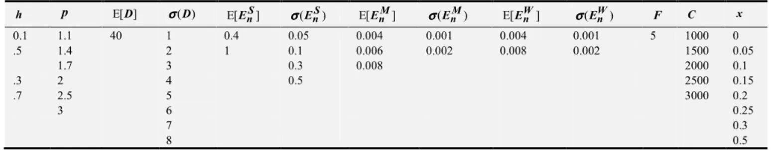
Table 2. Full factorial experiment design.
h p E[ ]D σσσσ( )D E[EnS] σσσσ(EnS) E[EnM] σσσσ(EnM) E[EnW] σσσσ(EWn ) F C x
0.1 1.1 40 1 0.4 0.05 0.004 0.001 0.004 0.001 5 1000 0
.5 1.4 2 1 0.1 0.006 0.002 0.008 0.002 1500 0.05
1.7 3 0.3 0.008 2000 0.1
.3 2 4 0.5 2500 0.15
.7 2.5 5 3000 0.2
3 6 0.25
7 0.3
h p E[ ]D σσσσ( )D E[EnS] σσσσ(EnS) E[EnM] σσσσ(EnM) E[EnW] σσσσ(EWn ) F C x
9 0.75
10 1
Before calculating the average values, we filter out all cases
where p < 0.5
p+h . The first reason for doing so is that if the
critical ratio is below 0.5, then it is optimal to stock less than the mean and if the standard deviation increases, then the optimal order quantity decreases [25]. The second reason is compliance with the numeric studies and results of Avrahami
et al. [3].
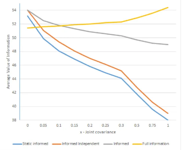
Figure 1 describes the dependence of the value of information and x. The figure is based on Tables 1 and 2. We see the value of information for factor h= 0.1 when x varies from 0 to 1. Note that a zero is not present in the vertical axis because it is less important in order to understand the behavior of different scenarios.
Figure 1. Value of Information by scenario – h=0.1.
We can clearly see that except for the value of full information, the value of information in all scenarios decreases as x increases. The reason for this is that the cost of the no information scenario does not increase significantly; however, the discrepancy between the modified demand and order quantity predicted by the scenarios accumulates over time. This discrepancy contributes to the high shortage costs and overall scenario cost, and finally, reduces the scenario’s value.
It is easy to understand the behavior of full information
when looking at variance equation 20. As x increases, the variance increases and, therefore, the cost of no information increases. The full information scenario, however, has a constant cost that causes the value of full information to increase with x. Note that Figure 1 s a numerical justification of our conjecture 1.1.
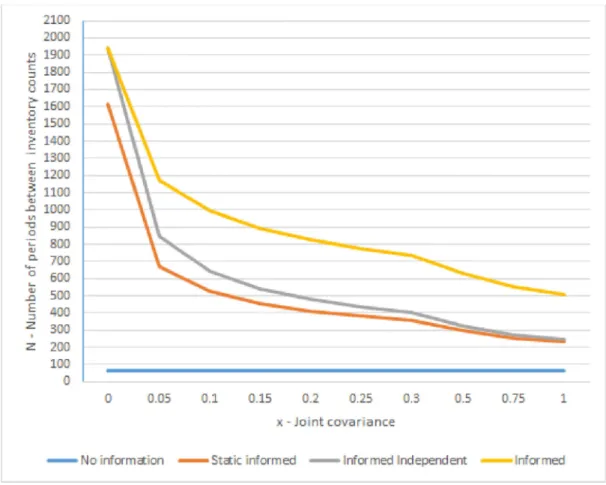
Figure 2. Stock review cycle by scenario – h=0.1.
6.3. Proactive Method Simulation
Parameter selection
We compare the performance of the proactive methods described in Chapter 0 by running a simulation of the no information scenario, IT stock reset and demand modification methods. Unlike the full factorial analysis with average-like results, here we focus on a single combination of problem parameters. We change only h and p , in order to manipulate the different cost factors, and run J= 1000 repetitions for each combination and each proactive method. In each repetition we calculate the period after which the
average cost starts to increase and the respective method cost. Thus, we get J random cost and period variables. Finally, we calculate the mean and standard deviation of the cost and number of periods until the inventory count.
To simulate the behavior of the scenario and the proactive methods, we need to generate multivariate normal realizations and this requires a positive definite covariance matrix. Unfortunately, the parameters that were presented earlier are not suitable here. Therefore, in Table 3 below, we present a new set of parameters that are used in all the simulations.
Table 3. Simulation parameters.
E[ ]D σσσσ( )D E[EnS] σσσσ(EnS) E[EnM] σσσσ(EnM) E[EWn ] σσσσ(EWn ) F C x
400 10 4 1 4 1 4 1 5 1000 0.3
The IT stock reset method is quite simple and does not require additional input or calibrations during runtime. After the realization of the demand and the error, if the available stock becomes negative, the IT stock is reset. All the regular costs are paid as usual. In the demand modification method, when shortage is observed, the mean demand parameter is modified upwards. The method requires a predefined modification factor. We see that a selection of this factor strongly effects the method performance. The mean demand
parameter is returned to the original value after the method reaches the inventory count period. Both methods decide that an inventory count is needed after the average period cost starts to increase.
6.4. Simulation Analysis
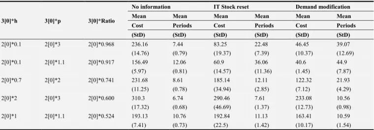
Table 4. Proactive methods of error correction.
3[0]*h 3[0]*p 3[0]*Ratio
No information IT Stock reset Demand modification Mean Mean Mean Mean Mean Mean Cost Periods Cost Periods Cost Periods (StD) (StD) (StD) (StD) (StD) (StD)
2[0]*0.1 2[0]*3 2[0]*0.968 236.16 7.44 83.25 22.48 46.45 39.07 (14.76) (0.79) (19.37) (7.39) (10.37) (12.69) 2[0]*0.1 2[0]*1.1 2[0]*0.917 156.49 12.06 60.9 36.06 40.6 44.9
(5.97) (0.81) (14.57) (11.36) (1.45) (7.87) 2[0]*0.7 2[0]*2 2[0]*0.741 231.68 8.61 185.14 12.11 122.32 21.93 (11.25) (0.78) (34.94) (2.85) (7.12) (4.29) 2[0]*2 2[0]*3 2[0]*0.600 310.3 6.74 290.46 7.61 233.08 10.56 (17.32) (0.68) (46.69) (1.37) (12.73) (0.98) 2[0]*1 2[0]*1.1 2[0]*0.524 193.13 10.76 192.84 11.13 163.41 10.59 (7.41) (0.73) (22.5) (1.42) (10.17) (1.54)
In this table we can see that both methods perform better than the no information scenario and demand modification performs better than IT stock reset. Nevertheless, the closer we are to the critical ratio of 0.5, the less improvement we have. In addition, we can see that IT stock reset has the highest standard deviation of cost. Critical ratios below 0.5 were also tested but the heuristics performed worse than the default no information scenario.
6.5. Statistical Justification
We want to compare two sample means, but before doing so, we need to test whether the sample variances are significantly different. Homoscedasticity is a very important assumption underlying the T test, because it influences the degrees of freedom of the test critical value. If the variances are different, we have to estimate each of them and, therefore, we have less degrees of freedom. To compare two variances we used the Fisher’s F test that divides the larger variance by the smaller
one. If the ratio is 1, the variances are the same. To be significantly different, the ratio should be significantly bigger than 1. To know if we should accept or decline the null hypothesis (that the two variances are not significantly different), we need to calculate the critical value of F. The degrees of freedom for the numerator as well as for denominator are calculated in the following way: df =n−1. If the calculated ratio is larger than the critical value, we reject the null hypothesis.
We performed this F test for all couples of our variables using the function var.test in R and, for each comparison, are results showed that all the variances (in each couple) are significantly different.
With these results in hand, we may proceed to performing the Student’s T test with the t.test function in R. Given that we already know that all the variances are significantly different, we use this function with the parameter var.equal=FALSE.
Table 5. T-test results: No information and IT stock reset.
h p Ratio t-value df p-value
0.1 3 0.968 129.7502 1883.479 p< 2.2 10⋅ −16
0.1 1.1 0.917 146.8987 1940.29 p< 2.2 10⋅ −16
0.7 2 0.741 31.7113 1568.931 p< 2.2 10⋅ −16
2 3 0.600 7.2456 1603.76 p= 6.66 10⋅ −13
1 1.1 0.524 -0.4256 1550.084 p= 0.6705
Table 6. T-test results: No information and demand modification.
h p Ratio t-value df p-value
0.1 3 0.968 192.2836 1319.329 p< 2.2 10⋅ −16
0.1 1.1 0.917 280.562 1037.919 p< 2.2 10⋅ −16
0.7 2 0.741 151.6659 1245.982 p< 2.2 10⋅ −16
2 3 0.600 71.5887 1487.807 p< 2.2 10⋅ −16
Table 7. T-test results: IT stock reset and demand modification.
h p Ratio t-value df p-value
0.1 3 0.968 49.2213 1505.76 p< 2.2 10⋅ −16
0.1 1.1 0.917 45.8193 1026.475 p< 2.2 10⋅ −16
0.7 2 0.741 52.6895 1077.463 p< 2.2 10⋅ −16
2 3 0.600 36.718 1173.663 p< 2.2 10⋅ −16
1 1.1 0.524 38.7981 1512.039 p< 2.2 10⋅ −16
In Table 5, we see that the combination of h= 1 and = 1.1
p yield a scenario where the difference between no information and IT stock reset is not statistically significant. This behavior is expected to be similar in cases where h≈ p and ratio ≈ 1.
From the Tables 6 and 7, we can conclude that in all cases except the one mentioned in the above paragraph, the difference between the methods is statistically significant with a confidence level of 95%.
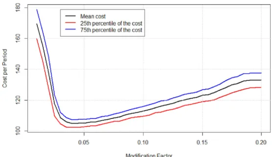
6.6. Modification Factor Selection
Since we saw that the demand modification method performs the best, we want to find the best modification factor. This factor is unique for each set of parameters so we could
select any combination of and that provide a critical ratio above 0.5. We chose and to test the performance close to 0.5, where we know it should be the least effective. We omit the standard deviation and focus on the mean value only.
Figure 3 was generated by running the demand modification method for ratios from 0 to 0.2 with a step of 0.01. The values of cost per period are averages of N= 100 simulations. We can see in Figure 3 that the optimal ratio is 0.04 and the respective cost is 104.5, which is a significant improvement over the corresponding value in Table 4. In addition, we can see the 25th and 75th percentile of the cost for each modification factor.
Figure 3. Modification factor selection.
7. Conclusions
In this work we concentrated on the value of information accuracy in a SC when working with an IT system. We extended the previously proposed models to consider correlations between inventory errors and demand. We added a new information scenario—the informed independent scenario, analyzed its behavior and compared its performance to other information scenarios. The correlation was modeled
using multivariate normal distribution. To improve the computation abilities, we rewrote the older tools in the R statistical language. We also optimized the tools for parallel computing, which allowed almost instant feedback. In addition, we provided two proactive methods of error corrections and showed, by a simulation, that they perform better than the default no information scenario. The results were tested using statistical t-test analysis to ensure they have the required significance level.
Clearly, it is worth investing in technology that would
h
p
= 1
provide visibility in supply chains. When real-time data is not available, however, we can construct statistical methods that can help overcome the discrepancy between the IT stock level and the actual stock. The effectiveness of these models will vary depending on the amount of data we assume.
In addition, when there is no available data to build the information scenarios models, we can rely on easy heuristics that perform better than the basic model.
References
[1] Atali, Aykut, Hau L Lee, and Özalp Özer. 2006. “If the inventory manager knew: Value of visibility and RFID under imperfect inventory information.” SSRN 1351606 http://ssrn.com/abstract=1351606.
[2] Kök, A Gürhan, and Kevin H Shang. 2007. “Inspection and replenishment policies for systems with inventory record inaccuracy.” Manufacturing and Service Operations Management 9 (2): 185–205.
[3] Avrahami, Assaf, Avinoam Tzimerman, Yale T. Herer, and Avraham Shtub. 2012. “The value of inventory accuracy in supply chain management.” Working Paper, Technion. [4] Lee, Hau, and Özalp Özer. 2007. “Unlocking the value of
RFID.” Production and Operations Management 16 (1): 40– 64.
[5] Sarac, Aysegul, Nabil Absi, and Stéphane Dauzère-Pérès. 2010. “A literature review on the impact of RFID technologies on supply chain management.” International Journal of Production Economics 128 (1): 77–95.
[6] Ha, Oh-Keun, Yong-Seok Song, Kyung-Yong Chung, Kang-Dae Lee, and Dongjoo Park. 2014. “Relation model describing the effects of introducing RFID in the supply chain: Evidence from the food and beverage industry in South Korea.”
Personal and Ubiquitous Computing 18 (3): 553–561. [7] Huber, Nicholas, and Katina Michael. 2007. “Vendor
perceptions of how RFID can minimize product shrinkage in the retail supply chain.” In RFID Eurasia, 2007 1st Annual, 1– 6. IEEE.
[8] [Fan et al. (2015)] Fan, Tijun, Feng Tao, Sheng Deng, and Shuxia Li. 2015. “Impact of RFID technology on supply chain decisions with inventory inaccuracies.” International Journal of Production Economics 159: 117–125.
[9] Gavirneni, Srinagesh, Roman Kapuscinski, and Sridhar Tayur. 1999. “Value of information in capacitated supply chains.”
Management Science 45 (1): 16–24.
[10] Cachon, Gérard P, and Marshall Fisher. 2000. “Supply chain inventory management and the value of shared information.”
Management Science 46 (8): 1032–1048.
[11] Lee, Hau L, Kut C So, and Christopher S Tang. 2000. “The value of information sharing in a two-level supply chain.”
Management Science 46 (5): 626–643.
[12] Moinzadeh, Kamran. 2002. “A multi-echelon inventory system with information exchange.” Management Science 48 (3): 414– 426.
[13] Gaukler, Gary M. 2011. “Item-level RFID in a retail supply chain with stock-out-based substitution.” Industrial Informatics, IEEE Transactions on 7 (2): 362–370.
[14] Ganesh, Muthusamy, Srinivasan Raghunathan, and Chandrasekharan Rajendran. 2014. “The value of information sharing in a multi-product, multi-level supply chain: Impact of product substitution, demand correlation, and partial information sharing.” Decision Support Systems 58: 79–94. [15] Sari, Kazim. 2015. “Investigating the value of reducing errors
in inventory information from a supply chain perspective.”
Kybernetes 44 (2): 176–185.
[16] Gaukler, Gary M, Ralf W Seifert, and Warren H Hausman. 2007. “Item-level RFID in the retail supply chain.” Production and Operations Management 16 (1): 65–76.
[17] Pelton, Lou E, Madhav Pappu, and Gary M Gaukler. 2010. “Preventing avoidable stockouts: The impact of item-level RFID in retail.” Journal of Business and Industrial Marketing
25 (8): 572–581.
[18] Chuang, Howard Hao-Chun, and Rogelio Oliva. 2015. “Inventory record inaccuracy: Causes and labor effects.”
Journal of Operations Management 39: 63–78.
[19] Iglehart, Donald L, and Richard C Morey. 1972. “Inventory systems with imperfect asset information.” Management Science 18 (8): B–388.
[20] DeHoratius, Nicole, Adam J Mersereau, and Linus Schrage. 2008. “Retail inventory management when records are inaccurate.” Manufacturing and Service Operations Management 10 (2): 257–277.
[21] Kök, A Gürhan, and Kevin H Shang. 2014. “Evaluation of cycle-count policies for supply chains with inventory inaccuracy and implications on RFID investments.” European Journal of Operational Research 237 (1): 91–105.
[22] Mersereau, Adam J. 2015. “Demand estimation from censored observations with inventory record inaccuracy.”
Manufacturing and Service Operations Management 17 (3): 335–349.
[23] Devore, J.L. 2011. Probability and Statistics for Engineering and the Sciences. Cengage Learning.
https://books.google.ca/books?id=3qoP7dlO4BUC.
[24] Lau, Hon-Shiang. 1997. “Simple formulas for the expected costs in the newsboy problem: An educational note.” European Journal of Operational Research 100 (3): 557–561.