Persistent Homology and Machine Learning
Primož Škraba
Artificial Intelligence Laboatory†, Jozef Stefan Institute E-mail: [email protected]
Keywords:persistent homology, topological data analysis, overview
Received:March 27, 2018
In this position paper, we present a brief overview of the ways topological tools, in particular persistent homology, has been applied to machine learning and data analysis problems. We provide an introduction to the area, including an explanation as to how topology may capture higher order information. We also provide numerous references for the interested reader and conclude with some current directions of rese-arch.
Povzetek: V tem ˇclanku predstavljamo pregled topoloških orodij, predvsem vztrajno homologijo, ki je upo-rabna na podroˇcju strojnega uˇcenja in za analizo podatkov. Zaˇcnemo z uvodom v podroˇcje in razložimo, kako topologija lahko zajame informacije višjega reda. ˇClanek vsebuje tudi reference na pomembna dela za zainteresiranega bralca. Zakljuˇcimo s trenutnimi smernicami raziskav.
1
Introduction
Topology is the mathematical study of spaces via connecti-vity. The application of these techniques to data is aptly na-med topological data analysis (TDA). In this paper, we pro-vide an overview of one such tool called persistent homo-logy. Since these tools remain unfamiliar to most computer scientists, we provide a brief introduction before providing some insight as to why such tools are useful in a machine learning context. We provide pointers to various successful applications of these types of techniques to problems where machine learning has and continues to be used.
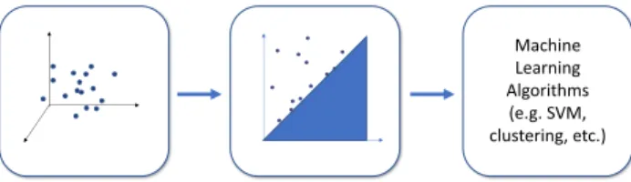
We begin with a generic TDA pipeline (Figure 1). The input is a set of samples, usually but not always embedded in some metric space. Based on the metric and/or additio-nal functions (such as density), a multiscale representation of the underlying space of data is constructed. This goes beyond considering pairwise relations to include higher-order information. Persistent homology is then applied. This is a tool developed from algebraic topology, which summarizes the whole multiscale representation compactly in the form of a persistence diagram. This compact repre-sentation can then be applied to various applications.
The goal of this paper is to provide a brief overview and introduce the main components in the TDA pipeline.
2
Simplicial complexes
Representations of the underlying space are built up simple pieces glued together. There are many different approaches to this, however the simplest is perhaps thesimplicial com-plex. Asimplexis the convex combination ofkpoints. A
†ARRS Project TopRep N1-0058
s s s
Machine Learning Algorithms (e.g. SVM, clustering, etc.)
Figure 1:The TDA pipeline - taking in a points in in sime metric space along with potentially other information, the data is turned into a compact representation called a persistence diagram. This summary can then be input into machine learning algorithms rat-her than the raw point cloud.
single point contains only itself, an edge is the convex com-bination of two points, three points make a triangle, four points a tetrahedron and so on (see Figure 2). More gene-rally, ak-dimensional simplex is the convex combination of(k+ 1)points. Just as an edge in a graph represents a pairwise relationship, triangles represent ternary relations-hips and higher dimensional simplices higher order relati-ons. A graph is an example of a one-dimensional complex, as it represents all pairwise information - all higher order information is discarded. As we include higher dimensi-onal simplices, we include more refined information yiel-ding more accurate models. Note that these models need to not exist in an ambient space (i.e. may not be embedded), but rather represents connectivity information. The geome-tric realization of simplicial complexes has a long history of study in combinatorics but we do not address it here.
Figure 2: Simplicies come in different dimension. From left to right, a vertex is 0-dim, an edge is 1-dim, a triangle 2-dim and a tetrahedron is 3-dim.
subset of data. The second is computation. As we consi-der higher orconsi-der relationships, there is often a combinato-rial blow-up as one must consider all k-tuples, leading to preprocessing requirements which are simply not feasible. The final obstacle is interpretability. While we can under-stand a simplex locally, underunder-standing the global structure becomes increasingly challenging.
This is the starting point for the tools we discuss below. Much of the effort of machine learning on graphs is trying to understand the qualitative properties of an underyling graph. This is often done by computing statistical features on the graph: degree distributions, centrality measures, di-ameter, etc. To capture higher order structure, we require a different set of tools. First, we note that a collection of simplices fit together. Just as in a graph, edges can only meet at an edge, simplices can only be glued together al-ong lower dimensional simplices, e.g. triangles meet alal-ong edges or at a vertex. This represents a constraint on how simple building blocks (e.g. simplices) can be glued toget-her to form a space. While this does not seriously limit the resulting spaces which can be represented, it does give us additional structure.
The starting point for the introduction is to describe the gluing map, called the boundary operator. For each k -simplex it describes the boundary as a collection ofk−1
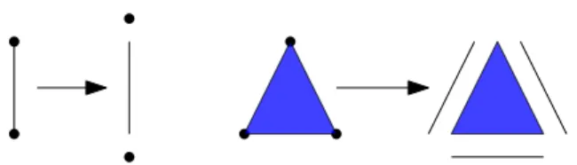
simplices. For example, the boundary of an edge consists of its two end points, the boundary of a triangle consists of its three edges (Figure 3). This can be represented as a matrix with the columns representing k-simplices and the rows k−1 simplices, which we denote ∂k. The k
-dimensionalhomologycan be defined as
Hk=
ker∂k
im∂k+1
The kernel is simply the collection ofk-simplices which form the nullspace of the matrix which correspond tocycles
(note that this agrees with the notion of graph-theoretic cy-cles). We the disregard all such cycles which bound regions filled-in by higher dimensional simplices. What remains is the numner of k-dimensional holes in the space. Spe-cifically, 0-dimensional homology corresponds to the num-ber of connected components, 1-dimensional homology the number of holes and so forth. Thek-th Betti number,βk
is the number of independent such features. This is analo-gous to the rank of a matrix describing the number of basis elements a vector space has. This yields a qualitative des-cription of the space. For a more complete introduction to homology, we recommend the book by Munkres [24] or the more advanced book by Hatcher[18]. An alternative
intor-Figure 3: Simplicies are glued together in a specific way with each simplex is glued to lower dimensional simplices, called its boundary. Here we show an edge has 2 verticies as its boundary and a triangle has three edges as its boundary.
duction which also includes persistent homology (descri-bed in the following section) can be found in Edlesbrunner and Harer[13]. Our goal here is to point out the intuition behind simplicial complexes and one approach to descri-bing them qualitatively. We do note that the algorithms and implementations are readily available [2, 19, 25, 23] and can often be interpreted through linear algebra.
3
Persistent homology
One problem with homology and topological features in general is that they are unstable. Adding a point to a space changes the number of components and the correspoding Betti number. This would make it seems as though this technique were not suitable for the study of data. A key insight from [14, 39], is that we need not look at a single space but rather a sequence of spaces, called afiltration. This is an increasing sequence of nested spaces, which ap-pears often when dealing with data.
∅ ⊆X0⊆X1⊆. . .⊆XN
For example a weighted graph can be filtered by the edge weights. Perhaps the most ubiquitous example is a finite metric space, where the space is a complete graph and the weights are distances. This occurs whenever the notion of a “scale" appears,Persistent homologyis the study of how qualitative features evolve over parameter choices. For ex-ample, the number of components is monotonically decre-asing as we connect points which are incredecre-asingly far away. This is in fact preciselysingle linkage clustering. Higher dimensional features such as holes can appear and disap-pear at different scales.
The key insight is that the evolution of features over pa-rameter choices can be encoded compactly in the form of a barcode or persistence diagram (Figure 4). We do not go into the algebraic reasons why this exists, rather we con-centrate on its implications. An active research area has been to extend this to higher dimensional parameter spaces [6, 22, 34], but has remained a challenging area. We refer the reader to [13] for introductions to persistent homology and its variants. For the next section, rather than consider a persistence diagram rather than a barcode. Here each bar is mapped to a point with the starting point of the bar as the
Consider a function on a simplicial complex, f :
K → R where we define the filtration as the sublevel
set f−1(−∞, α]. That is, we include all simplices with
a lower function value. As we increaseα, the set of sim-plicies with a lower function value only grows, hence we only add simplices. Therefore, we obtain an increasing sequence of topological spaces, i.e. a filtration. Define
Xα:=f−1(−∞, α], then
Xα1⊆Xα2 ⊆ · · · ⊆Xαn α1≤α2≤ · · · ≤αn
As another example in a metric space, we include all edges which represent a distance less thanα. Consider a pertur-bed metric space, giving rise to a different functiong. The following theorem establishes stability - that if the input (in this case, the function) does not change much, the output should not change much.
Theorem 1([11]). LetKbe two simplicial complexes with two continuous functionsf, g: X →R. Then the
persis-tence diagramsDgm(f)andDgm(g)for their sublevel set filtrations satisfy
dB(Dgm(f),Dgm(g)))≤ ||f−g||∞.
whereDgm(·)represents the persistence diagram (i.e. a topological descriptor which is a set of points inR2) and
dB(·)represents bottleneck distance. This is the solution
to the optimization which constructs a matching between the points in two diagrams which minimizes the maximum distance between matched points. While it is difficult to overstate the importance of this result, it does have some drawbacks. In particular the bound is in terms of the∞ -norm which in the presence of outliers can be very large. Recently this result has been specialized to Wasserstein sta-bility, which is a much stronger result (albeit in a more li-mited setting).
Theorem 2([36]). Letf, g : K → Rbe two functions.
ThenWp(Dgm(f),Dgm(g))≤ kf−gkp.
Wasserstein distance is common in the machine learning and statistics literature as it is a natural distance between probability distributions. This recent result indicates that the distances between diagrams is indeed more generally stable and so suitable for applications. Stability has be-come an area of study in its own right and we now have a good understanding of the types of stabilty we can expect. The literature is too vast to list here so we limit ourselves to a few relevant pointers [3, 8].
4
Topological features
Here we describe some applications of persistence to ma-chine learning problems. The key idea is to use persistence diagrams as feature vectors as input further machine lear-ning algorithms, There are several obstacles to this. The most important is that the space of persistence diagrams is quite pathological. The first approach to move around
this arepersistence landscapes[4]. This lifts persistence diagrams into a Hilbert space which allows them to be fed into most standard machine learning algorithms. This has been followed up by rank functions [33], as well as several kernels [30], More recently, there has been work on lear-ning optimal functions of persistence diagrams using deep learning [20].
There has also been significant work on the statistical properties of persistence diagrams and landscapes [16], in-cluding bootstrapping techniques [9].
These techniques have been applied to a number of ap-plication areas. Perhaps most extensive is in geometry pro-cessing. Combined with local features such as curvature or features based on heat kernels, different geoemtric struc-ture can be extracted including symmetry [26], segmenta-tion [35], and shape classificasegmenta-tion and retrival [7].
Another application area where persistence diagrams have been found to be informative are for biology, especi-ally for protein docking [1] and modelling pathways in the brain [17]. The final application area we mention is ma-terial science. This is an area where machine learning has not yet been applied extensively. Partially due to the fact that the input is of a significantly different flavor than that which is typical in machine learning. For example, stan-dard image processing techniques do not work well with scientific images such as electron microscope images. By using topological summaries, the relevant structure is well-captured [32, 21]. This area is still in the early stages with many more exciting developments expected.
We conclude this section by noting that persistence di-agrams are not the only topological features which have been applied. Originally, the Euler curvewas applied to fMRIs [38]1. This feature has been extensively studied in
the statistics literature, but is provably less informative than persistence diagrams - although it is far more computatio-nally tractable. In addition to fMRI, it has been applied to various classification problems [31].
5
Other applications
In additon to providing a useful summary and features for machine learning algorithms, a second direction of inte-rest is the map back to data. This inverse probelm is very difficult and can often be impossible in general. Nonethe-less, the situation is often not as hopeless as it would seem. Some of the first work in this direction is re-interpreting single linkage clustering through the lens of persistence [10]. While it is well known that single linkage clusters are unstable, it is possible to use persistence to show that there exist stable parts of the clusters and a “soft" clustering al-gorithm can be developed to stabilize clusters, where each data point is assigned a probability that it is assigned to a given cluster. A current direction of research is to find simi-lar stable representations in the data for higher dimensional structures (such as cycles).
0 0.1 0.2 0.3 0.4 0.5 0.6 0.7 0
0.1 0.2 0.3 0.4 0.5 0.6 0.7
-1.5 -1 -0.5 0 0.5 1 1.5
-1.5 -1 -0.5 0 0.5 1 1.5
0 0.01 0.02 0.03 0.04 0.05 0.06 20
40 60 80 100 120 140 160 180
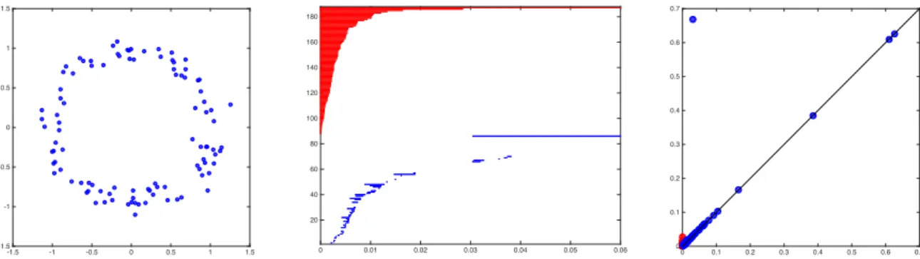
Figure 4: Persistence in a nutshell. Given input points (left), we compute a barcode (middle). which shows how long features live. The red shows the lifetimes of when components merge, while the blue bars show 1-dimensional holes. We can map each bar to a point by taking the start and end as thexandycoordinates respectively giving us the persistence diagram (right). Here we see that the big whole in the middle of the data set appears as a prominent feature (the blue dot far from the diagonal on the right).
A related problem is one of parameterization. That is, find intrinsic coordinates describing the data, extending successful techniques in dimensionality reduction, This in-cludes linear methods such as PCA and MDS as well as non-linear methods such as ISOMAP and LLE. The first such work coordinizaed the space of textures using a Klein bottle as the underlying model [28] - a topological model found a few years prior [5]. This was however built by hand. The first class of general methods is first to map ci-crular coordinates to data [12]. This is particularly useful when dealing with recurrence in time-varying systems. Re-currence (including periodicity) is naturally modeled by an angle, Combining persistence with least-squares optimiza-tion provides an automatic pipeline to finding such coor-dinates. This was applied to characterizing human moti-ons such as different walks and other activities [37]. Furt-her work has shown how to construct coordainte systems for higher dimensional structures based on the projective plane [27].
The final direction we consider is to encode topological constraints in machine learning algorithms. In [29] topo-logical priors were used to aid in parameter selection. For example, the reconstruction of a racetrack should have one component and one hole (the main loop). Computing the persistence with respect to a reconstruction parameter (e.g. bandwith of a kernel) can allow us to choose a parameter value where the reconstruction has the desired topological “shape." The encoding of topological constraints is still in the very early stages but has the potential to provide a new type of regularization to machine learning techniques.
6
Discussion
Topological data analysis and applications of topology are still in their early stages. Various efforts to bridge the gap between algebraic topology and statistics (and probability) has made rapid progress over the last few years which has culminated in a dedicated R-package [15]. At the same time, increasingly efficient software exists for computing persistent homology exists, where now it is feasible to
con-sider billions of points in low dimensions. This is increa-singly bridging the gap between theory and practice.
The area has undergone rapid development over the last 10 years and is showing no signs of slowing down. In terms of theory, the primary question drinving the community is the notion of multi-dimensional or multi-parameter persis-tence, where the computational obstacles are much more daunting. Nonetheless, progress is being made. Success promises to further reduce the need and dependence on pa-rameter tuning.
The combination of deep learning techniques with to-pological techniques promises to provide new areas of ap-plications as well as potentially performance. These met-hods are primarily complementary allowing them to build on each other. In conclusion, while obstacles remain, the inclusion of topological techniques into the machine lear-ning toolbox is rapidly making progress.
References
[1] Pankaj K Agarwal, Herbert Edelsbrunner, John Ha-rer, and Yusu Wang. Extreme elevation on a 2-manifold.Discrete & Computational Geometry, 36(4):553–572, 2006.
[2] U Bauer. Ripser. https://github.com/Ripser/ripser, 2016.
[3] Ulrich Bauer and Michael Lesnick. Induced matc-hings of barcodes and the algebraic stability of per-sistence. InProceedings of the thirtieth annual sym-posium on Computational geometry, page 355. ACM, 2014.
[4] Peter Bubenik. Statistical topological data analysis using persistence landscapes.The Journal of Machine Learning Research, 16(1):77–102, 2015.
[6] Gunnar Carlsson and Afra Zomorodian. The theory of multidimensional persistence.Discrete & Com-putational Geometry, 42(1):71–93, 2009.
[7] Frédéric Chazal, David Cohen-Steiner, Leonidas J Guibas, Facundo Mémoli, and Steve Y Oudot. Gromov-hausdorff stable signatures for shapes using persistence. In Computer Graphics Forum, vo-lume 28, pages 1393–1403. Wiley Online Library, 2009.
[8] Frédéric Chazal, Vin De Silva, Marc Glisse, and Steve Oudot. The structure and stability of persistence mo-dules.arXiv preprint arXiv:1207.3674, 2012.
[9] Frédéric Chazal, Brittany Terese Fasy, Fabrizio Lecci, Alessandro Rinaldo, Aarti Singh, and Larry Wasser-man. On the bootstrap for persistence diagrams and landscapes.arXiv preprint arXiv:1311.0376, 2013.
[10] Frédéric Chazal, Leonidas J Guibas, Steve Y Oudot, and Primoz Skraba. Persistence-based clustering in riemannian manifolds. Journal of the ACM (JACM), 60(6):41, 2013.
[11] David Cohen-Steiner, Herbert Edelsbrunner, and John Harer. Stability of persistence diagrams. Dis-crete & Computational Geometry, 37(1):103– 120, 2007.
[12] Vin De Silva, Dmitriy Morozov, and Mikael Vejdemo-Johansson. Persistent cohomology and ci-rcular coordinates. Discrete & Computational Geometry, 45(4):737–759, 2011.
[13] Herbert Edelsbrunner and John Harer.Computational topology: an introduction. American Mathematical Soc., 2010.
[14] Herbert Edelsbrunner, David Letscher, and Afra Zo-morodian. Topological persistence and simplification. InFoundations of Computer Science, 2000. Procee-dings. 41st Annual Symposium on, pages 454–463. IEEE, 2000.
[15] Brittany Terese Fasy, Jisu Kim, Fabrizio Lecci, and Clément Maria. Introduction to the r package tda.
arXiv preprint arXiv:1411.1830, 2014.
[16] Brittany Terese Fasy, Fabrizio Lecci, Alessandro Ri-naldo, Larry Wasserman, Sivaraman Balakrishnan, Aarti Singh, et al. Confidence sets for persistence di-agrams. The Annals of Statistics, 42(6):2301–2339, 2014.
[17] Margot Fournier, Martina Scolamiero, Mehdi Gholam-Rezaee, Hélène Moser, Carina Ferrari, Philipp S Baumann, Vilinh Tran, Raoul Jenni, Luis Alameda, Karan Uppal, et al. M3. topological analyses of metabolomic data to identify markers of early psychosis and disease biotypes. Schizophrenia Bulletin, 43(suppl_1):S211–S212, 2017.
[18] Allen Hatcher.Algebraic topology. 2002.
[19] Gregory Henselman and Robert Ghrist. Matroid filtrations and computational persistent homology.
arXiv preprint arXiv:1606.00199, 2016.
[20] Christoph Hofer, Roland Kwitt, Marc Niethammer, and Andreas Uhl. Deep learning with topological sig-natures. InAdvances in Neural Information Proces-sing Systems, pages 1633–1643, 2017.
[21] Yongjin Lee, Senja D Barthel, Paweł Dłotko, S Mo-hamad Moosavi, Kathryn Hess, and Berend Smit. Quantifying similarity of pore-geometry in nanopo-rous materials.Nature Communications, 8, 2017.
[22] Michael Lesnick. The theory of the interlea-ving distance on multidimensional persistence mo-dules. Foundations of Computational Mathematics, 15(3):613–650, 2015.
[23] Dmitriy Morozov. Dionysus. Software available at http://www. mrzv. org/software/dionysus, 2012.
[24] James R Munkres. Elements of algebraic topology, volume 4586. Addison-Wesley Longman, 1984.
[25] Vidit Nanda. Perseus: the persistent homology soft-ware. Software available at http://www. sas. upenn. edu/˜ vnanda/perseus, 2012.
[26] Maks Ovsjanikov, Quentin Mérigot, Viorica P˘atr˘au-cean, and Leonidas Guibas. Shape matching via quotient spaces. InComputer Graphics Forum, vo-lume 32, pages 1–11. Wiley Online Library, 2013.
[27] Jose A Perea. Multi-scale projective coordinates via persistent cohomology of sparse filtrations.arXiv pre-print arXiv:1612.02861, 2016.
[28] Jose A Perea and Gunnar Carlsson. A klein-bottle-based dictionary for texture representation. Internati-onal journal of computer vision, 107(1):75–97, 2014.
[29] Florian T Pokorny, Carl Henrik Ek, Hedvig Kjell-ström, and Danica Kragic. Topological constraints and kernel-based density estimation. Advances in Neural Information Processing Systems, 25, 2012.
[30] Jan Reininghaus, Stefan Huber, Ulrich Bauer, and Ro-land Kwitt. A stable multi-scale kernel for topological machine learning. InProceedings of the IEEE con-ference on computer vision and pattern recognition, pages 4741–4748, 2015.
[31] Eitan Richardson and Michael Werman. Efficient classification using the euler characteristic. Pattern Recognition Letters, 49:99–106, 2014.
[32] Vanessa Robins, Mohammad Saadatfar, Olaf Delgado-Friedrichs, and Adrian P Sheppard. Per-colating length scales from topological persistence analysis of micro-ct images of porous materials.
[33] Vanessa Robins and Katharine Turner. Principal com-ponent analysis of persistent homology rank functi-ons with case studies of spatial point patterns, sphere packing and colloids. Physica D: Nonlinear Pheno-mena, 334:99–117, 2016.
[34] Martina Scolamiero, Wojciech Chachólski, Anders Lundman, Ryan Ramanujam, and Sebastian Öberg. Multidimensional persistence and noise. Founda-tions of Computational Mathematics, 17(6):1367– 1406, 2017.
[35] Primoz Skraba, Maks Ovsjanikov, Frederic Chazal, and Leonidas Guibas. Persistence-based segmen-tation of deformable shapes. In Computer Vision and Pattern Recognition Workshops (CVPRW), 2010 IEEE Computer Society Conference on, pages 45–52. IEEE, 2010.
[36] Primoz Skraba and Katharine Turner. Wasserstein sta-bility of persistence diagrams. submitted to the Sym-posium of Computational Geometry 2018.
[37] Mikael Vejdemo-Johansson, Florian T Pokorny, Pri-moz Skraba, and Danica Kragic. Cohomological lear-ning of periodic motion.Applicable Algebra in Engi-neering, Communication and Computing, 26(1-2):5– 26, 2015.
[38] Keith J Worsley, Sean Marrett, Peter Neelin, Alain C Vandal, Karl J Friston, Alan C Evans, et al. A uni-fied statistical approach for determining significant signals in images of cerebral activation.Human brain mapping, 4(1):58–73, 1996.