Vol. 12, No. 3, 2019, 1215-1230 ISSN 1307-5543 – www.ejpam.com Published by New York Business Global
Convergence of an exponential Runge–Kutta method
for non-smooth initial data
Muhammad Asif Gondal1,∗, Inayatur Rehman1, Asima Razzaque2
1 Department of Mathematics and Sciences, Dhofar University, Salalah, Oman 2 Department of Mathematics, University of Education, Lahore, Pakistan
Abstract. The paper presents error bounds for the second order exponential Runge-Kutta method for parabolic abstract linear time-dependent differential equations incorporating non-smooth initial data. As an example for this particular type of problems, the paper presents a spatial discretization of a partial integro-differential equation arising in financial mathematics, where non-smooth initial conditions occur in option pricing models. For this example, numerical studies of the convergence rate are given.
2010 Mathematics Subject Classifications: 35K90
Key Words and Phrases: Exponential integrators, Runge–Kutta methods, Integro-differential equations
1. Introduction
To give numerical solution of stiff differential equations, exponential integrators have been constructed. Through Exponential integrators, unlike standard numerical integra-tors, the exponential and related functions (often called ϕ-functions) of large matrices can be used explicitly. The exponential Runge-Kutta methods of collocation type have been constructed by Hochbruck & Ostermann [9] and their convergence properties were analyzed for linear and semi-linear parabolic problems . Hochbruck & Ostermann [8] also studied explicit exponential Rung-Kutta methods for the time integration of semi-linear parabolic problems. Gondal [4] considered exponential Rosenbrock integrators for option pricing. Different types of exponential integrators and their applications are discussed in details in [6, 10, 11, 18, 19].
Henry [7] and Pazy [16] studied semi-linear problems and contributed significantly. Le Roux [17] introduced for the first time non-smooth data error estimates for time dis-cretizations of linear parabolic problems. The error bounds for time disdis-cretizations of
∗
Corresponding author.
DOI: https://doi.org/10.29020/nybg.ejpam.v12i3.3423
Email addresses: [email protected](M. A. Gondal),
[email protected](I. Rehman),[email protected] (A. Razzaque)
semi-linear parabolic equations with non-smooth initial data have been inferred in [12]. Linearly implicit time discretization of semi-linear parabolic equations with non-smooth initial data was studied by the authors in [15]. In [5], author proved convergence result of an exponential Euler method using non-smooth initial data for option pricing. We mean to examine convergence properties of exponential Runge-Kutta method for linear parabolic problems that spring up in financial problems. To evaluate this, we cultivate in an abstract Banach space framework of sectorial operators and analytic semi-groups and prove convergence for Exponential Runge-Kutta method for non-smooth initial data.
The jump diffusion model, proposed in [14], is chosen as an application of our analysis. In particular, we discuss the partial integro-differential equations(PIDE) for Mertons model. Briani, La Chioma & Natalini [13] used an explicit method to solve Mertons model and constituted a convergence theory for explicit schemes for varied integro-differential Cauchy problems. Cont & Voltchkova [2] used implicit-explicit finite difference methods success-fully for European and barrier options in jump diffusion and exponential Levy models. In a paper [3], one can find different option pricing problems solved numerically through Chebychev discretisation schemes and exponential integrators.
This article is attributed to a theoretical convergence analysis of exponential integrators which is transported out within the framework of evolution equations in Banach spaces.In financial applications, the initial information is generally non-smooth and lies of the payoff function of the option. Therefore, in case of non-smooth initial data, the matter of concern is to have practical error bounds. A bound of this nature is developed in [5] of order one for the exponential Euler method. Following, in Section 3, a error bound is established for the method called an exponential RungeKutta method of order two, and the result is given in Theorem 1.
Besides this preamble, the paper comprises of four sections. Section 2 describes the expo-nential Rung-Kutta and expoexpo-nential Euler time integrators. Section 3 present the main results and originate new error bounds. Although in case of non-smooth initial data, error bounds derived in [12] and [15]. But the results for exponential integrators, however, have not been experienced. For the application of analysis, Section 4 offers an example from the Mertons models. The Conclusion includes few final remarks.
2. Numerical method
In this section,the abstract form of evaluation equation that results from partial integro-differential equations, that arise in financial mathematics, is considered as follows:
u0(t) =Au(t) +Bu(t) +g(t), u(t0) =u0, 0< t≤T, (1)
The variation-of-constants formula with the exact solution representation of (1) is
u(tn+1) = ehAu(tn) +
Z h
0
e(h−τ)AB·u(tn+τ)dτ +
Z h
0
e(h−τ)Ag tn+τ
The approximation obtained through the left rectangular rule is
u(tn+1)≈ehAu(tn) +
Z h
0
e(h−τ)AB·u(tn)dτ+
Z h
0
e(h−τ)Ag tn
dτ
and
un+1 = ehAun+hϕ1(hA)(Bun+g(tn)), ϕ1(hA) =
1 h
Z h
0
e(h−τ)Adτ. (2)
which is known as the exponential Euler method of order one for problem given in (1). Now for (1), we assume the following exponential Runge–Kutta methods
un+1 = ehAun+h s
X
i=1
bi(hA) Buni+g(tn+cih)
, (3)
uni = ecihAun+h i−1
X
j=1
aij(hA) Bunj+g(tn+cjh)
, 1≤i≤s.
The exponential Runge–Kutta method (3) for a second-order method with two stages can be written as
un+1 = ehAun+h
b1(hA) Bun1+g(tn+c1h)
+ b2(hA) Bun2+g(tn+c2h)
, (4)
un1 = ec1hAun,
un2 = ec2hAun+ha21(hA) Bun1+g(tn+c1h)
.
Further we know that for a second-order method with two stages it must satisfy the following three order conditions given in Hochbruck & Ostermann [9]
b1(hA) +b2(hA) = ϕ1(hA),
c1b1(hA) +c2b2(hA) = ϕ2(hA), (5)
a21(hA) = c2ϕ1(c2hA),
where
ϕ1(z) =
ez−1
z , ϕ2(z) =
ϕ1(z)−1
z .
By taking c1 = 0 and c2 = 1, we find the values of b1 =ϕ1(hA)−ϕ2(hA), b2 = ϕ2(hA)
and a21=ϕ1(hA). Hence we can write (4) as
un+1 = ehAun+h(ϕ1(hA)−ϕ2(hA))Bun1+hϕ2(hA)Bun2
+ h(ϕ1(hA)−ϕ2(hA))g(tn) +hϕ2(hA)g(tn+h), (6)
un1 = un,
un2 = ehAun+hϕ1(hA) Bun1+g(tn)
. (7)
3. Convergence of an exponential Runge–Kutta method of order two for non-smooth initial data
In this section we study an exponential Runge–Kutta method of order two for dis-cretizing an abstract problem (1) in time. OnA, B and g, our assumptions are the same as given in Gondal [5].
Now first we are going to prove vital properties of the exact solution and then we will move to the numerical solution.
Lemma 1. Assume that problem (1) fulfill the hypotheses of Lemma 2 given in Gondal [5]. Then the bounds
kL−1u00(t)k ≤ C
t , on (0, T], (8)
hold uniformly on 0≤t≤T for non-smooth initial data.
Proof. From Lemma 2 given in Gondal [5] we use equation (18) given in Gondal [5] in
u00(t) =Lu0(t) +g0(t), (9)
and we get
u00(t) =L2etLu0+LetLg(0) + etLg0(0) +tϕ1(tL)g00(0) +. . . . (10)
Premultiplying withL−1 on both sides of (10), we get
L−1u00(t) =LetLu0+ etLg(0) +. . . (11)
Now multiplying with ton both sides of (11), we have
tL−1u00(t) =tLetLu0+tetLg(0) +. . . (12)
Therefore
ktL−1u00(t)k ≤C or kL−1u00(t)k ≤ C
t. (13)
In this section, we will also derive error bounds for exponential Runge–Kutta dis-cretizations of (1). The exponential Runge–Kutta method of order two for given problem is (6). To analyze (6), one can write the exact solution of (1) as
u(tn+1) = ehAu(tn) +
Z tn+1
tn
e(tn+1−τ)ABu(τ)dτ+
Z tn+1
tn
e(tn+1−τ)Ag(τ)dτ. (14)
To write (14) in the form of (6), below result will be helpful
Z tn+1
tn
e(tn+1−τ)Adτ =
Z h
0
e(h−s)Ads=hϕ1(hA) (15)
Z tn+1
tn
e(tn+1−τ)A(τ−t n)dτ =
Z h
0
Theorem 1. Assume that problem (1) fulfill the hypotheses of Lemma 2 given in Gondal [5] and that AB = BA. For the numerical solution, we consider the exponential Runge-Kutta method (6). Also suppose thatg0,g00are bounded andg: [0, T]→ X is differentiable. Then the following error bound
ku(tn)−unk ≤ Ch2
tn
(|logh|+1) (17)
holds uniformly in 0≤tn≤T for non-smooth initial data.
Proof. We can write the difference between the gterms from (14) and (6) as
n+1(g) =
Z tn+1
tn
e(tn+1−τ)Ag(τ)dτ −h(ϕ
1(hA)−ϕ2(hA))g(tn)
− hϕ2(hA)g(tn+h). (18)
Using results (15) and (16) in (18) and simplifying, we get
n+1(g) =
Z tn+1
tn
e(tn+1−τ)Ag(τ)−g(t n) +
τ −tn h g(tn)
− τ−tn
h g(tn+h)
dτ. (19)
By using Taylor series we can write
g(τ) =g(tn) + (τ−tn)g0(tn) +
1
2(τ −tn)
2g00(t
n) +. . . (20)
g(tn+h) =g(tn) +hg0(tn) + h2
2 g
00(t
n) +. . . . (21)
Now substitute g(τ) andg(tn+h) from equations (20) and (21) in (19) and after
simpli-fication and neglecting higher order terms we can write (19) as
n+1(g) =
Z tn+1
tn
e(tn+1−τ)A(τ−tn) 2
2 −
h(τ−tn)
2
g00(tn)dτ,
kn+1(g)k ≤
Z tn+1
tn
ke(tn+1−τ)Ak
(τ −tn)2
2 −
h(τ −tn)
2 kg
00
(tn)kdτ,
≤ C
Z tn+1
tn
(τ−tn)2
2 +
h(τ −tn)
2
dτ,
≤ Ch
3
6 +C h3
2 =Ch
3. (22)
This is the one way to solve (19) in which we have to assume that all higher order deriva-tives of g are bounded. There is another good and tricky way to prove that n+1(g) is
bounded. For this trick, we can writeg(τ) instead of Taylor series in the following form
g(τ) = g(tn) +
Z τ
tn
= g(tn) +
Z τ
tn
1·g0(s)ds,
= g(tn) +
Z τ
tn
(s−τ)0g0(s)ds. (23)
Integration by part yields
g(τ) = g(tn) + (τ−tn)g0(tn) +
Z τ
tn
(τ−s)g00(s)ds, (24)
since we can writeg(tn+h) =g(tn+1). Using (24), one can write
g(tn+1) = g(tn) + (tn+1−tn)g0(tn) +
Z tn+1
tn
(tn+1−s)g00(s)ds,
= g(tn) +hg0(tn) +
Z tn+1
tn
(tn+1−s)g00(s)ds. (25)
Now we can use expressions (24) and (25) forg(τ) and g(tn+h) instead of (20) and (21)
in (19) to get (22). In this case we only assume that first and second order derivatives of g are bounded.
Now in the same way we can write the difference between the u terms from (14) and (6) as
n+1(u) =
Z tn+1
tn
e(tn+1−τ)ABu(τ)dτ−h(ϕ
1(hA)−ϕ2(hA))Bun
− hϕ2(hA)Bun2, (26)
since we can write Z tn+1
tn
e(tn+1−τ)ABu(τ)dτ =
Z tn+1
tn
e(tn+1−τ)AB
u(tn)− τ−tn
h u(tn) + τ −tn
h u(tn+h)
+ u(τ)−u(tn) + τ −tn
h u(tn)− τ −tn
h u(tn+h)
dτ = hϕ1(hA)Bu(tn)−hϕ2(hA)Bu(tn) +hϕ2(hA)Bu(tn+1)
+
Z tn+1
tn
e(tn+1−τ)AB
u(τ)−u(tn) + τ−tn
h u(tn)
− τ −tn
h u(tn+h)
dτ. (27)
Using (27) in (26) and simplifying, we have
n+1(u) = hϕ1(hA)B(u(tn)−un)−hϕ2(hA)B(u(tn)−un)
+ hϕ2(hA)B(u(tn+1)−un2) +Rn+1,
where
Rn+1=
Z tn+1
tn
e(tn+1−τ)AB
u(τ)−u(tn) + τ −tn
h u(tn)− τ−tn
h u(tn+h)
dτ. (29)
Since one can write
u(tn+1)−un2 = u(tn+1)−un+1+un+1−un2,
= n+1+un+1−un2,
ku(tn+1)−un2k ≤ kn+1k+kun+1−un2k. (30)
Now from (6) and (7) we can write
un+1−un2 = hϕ2(hA)B(un2−un) +hϕ2(hA)(g(tn+h)−g(tn)),
kun+1−un2k ≤ Chkun2−unk+Ch2, (31)
sincekg(tn+h)−g(tn)k ≤Ch. Now
un2−un = un2−un+1+un+1−un,
kun2−unk ≤ kun+1−unk+kun+1−un2k. (32)
From (6) we can write forn≥1
un+1−un = ehAun−un+O(h),
= (ehA−1)un+O(h) =hAϕ1(hA)un+O(h),
= hAϕ1(hA)(u(tn) +n) +O(h), since un=u(tn) +un−u(tn),
= hAϕ1(hA)n+hAϕ1(hA)u(tn) +O(h),
kun+1−unk ≤ Cknk+Ch·
C tn
+O(h), (33)
sincekAu(tn)k ≤ tCn forn >0.
Using (33) in (32) and then (32) in (31) yields
kun+1−un2k ≤ Chkun+1−un2k+Chknk+Ch2·
1 tn
+Ch2,
(1−hC)kun+1−un2k ≤ Chknk+Ch2·
1 tn
+Ch2, (34)
h small gives thathC ≤ 1
2, therefore for n≥1
kun+1−un2k ≤Chknk+ Ch2
tn
+Ch2. (35)
Using (35) in (30) and then (30) in (28) gives for n≥1
kn+1(u)k ≤ Chknk+Chkn+1k+Ch2knk+
+ Ch3+kRn+1k. (36)
Forn= 0, we use (30) to obtain
ku(t1)−u02k ≤ k1k+ku1−u02k,
with the help of (31), we get
ku(t1)−u02k ≤ k1k+Chku02−u0k+Ch2. (37)
As
ku02−u0k ≤ ku02k+ku0k ≤C, (38)
Using (38) in (37) and then (37) in (28) gives for n= 0
k1(u)k ≤ Chk0k+Chk1k+Ch2+Ch3+kR1k. (39)
Now we want to prove kRn+1kis bounded. For this, we can writeu(τ) andu(tn+1) by
using the same concept of (24) in the following form
u(τ) =u(tn) + (τ −tn)u0(tn) +
Z τ
tn
(τ −s)u00(s)ds, (40)
u(tn+1) =u(tn) +hu0(tn) +
Z tn+1
tn
(tn+1−s)u00(s)ds. (41)
Substituting the expressions foru(τ) from (40) andu(tn+h) =u(tn+1) from (41) in (29)
and simplifying, we get
Rn+1 =
Z tn+1
tn
e(tn+1−τ)AB
Z τ
tn
(τ−s)u00(s)ds−τ−tn
h
Z tn+1
tn
(tn+1−s)u00(s)ds
dτ. (42)
Rn+1=Rn+1,2+Rn+1,3 (43)
where
Rn+1,2=
Z tn+1
tn
e(tn+1−τ)AB
Z τ
tn
(τ −s)u00(s)ds
dτ, (44)
and
Rn+1,3 =
Z tn+1
tn
e(tn+1−τ)AB
τ −tn
h
Z tn+1
tn
(tn+1−s)u00(s)ds
dτ. (45)
Now to solve (44), we use the identityAA−1 =I and get
Rn+1,2 =
Z tn+1
tn
e(tn+1−τ)AB
Z τ
tn
(τ −s)AA−1u00(s)ds
dτ. (46)
A can commute withB, i.e., AB=BA, ifB is a convolution integral, therefore
Rn+1,2 = A
Z tn+1
tn
e(tn+1−τ)AB
Z τ
tn
(τ−s)A−1u00(s)ds
Since
n+1 = u(tn+1)−un+1,
= ehAn+n+1(g) +n+1(u). (48)
Therefore from (6) and (14) and using (22) and (36), we get from (48) the error recursion forn >0
kn+1k ≤ kehAkknk+Chknk+Chkn+1k+Ch2knk
+ Ch
3
tn
+Ch3+kRn+1k.
(49)
h small gives thathC ≤ 1
2, therefore
kn+1k ≤ CkehAkknk+Chknk+Ch2knk+
Ch3 tn
+Ch3+kRn+1k,
.. .
knk ≤ CkenhAkk0k+Ch
n−1
X
j=0
ke(n−j−1)hAkkjk+Ch2 n−1
X
j=0
ke(n−j−1)hAkkjk
+ Ch3 n−1
X
j=1
ke(n−j−1)hAkk1
tj
k+Ch2+Ch3
n−1
X
j=0
ke(n−j−1)hAk
+
n−1
X
j=0
ke(n−j−1)hARj+1k. (50)
Using Lemma 2 given in Gondal [5] and fact that tj =jh, we get
knk ≤ Ck0k+Ch
n−1
X
j=0
kjk+Ch2 n−1
X
j=0
kjk+Ch2 n−1
X
j=1
k1
jk+Ch
3·n
+
n−1
X
j=0
ke(n−j−1)hARj+1k. (51)
Since we know thatnh=T,Ch2 ≤Ch and k0k= 0, and using the result (??), we get
knk ≤ Ch
n−1
X
j=0
kjk+Ch2(C+|logh|) +Ch2T + n−1
X
j=0
ke(n−j−1)hARj+1k,
≤ Ch
n−1
X
j=0
kjk+Ch2(1+|logh|) + n−1
X
j=0
After this, it is proved that Pn−1
j=0ke(n−j−1)hARj+1k is bounded. For this we can write n−1
X
j=0
ke(n−j−1)hARj+1k= n−1
X
j=0
ke(n−j−1)hARj+1,2k+ n−1
X
j=0
ke(n−j−1)hARj+1,3k. (53)
From (47) we can write
Pn−2
j=1 ke
(n−j−1)hAR
j+1,2k (54)
=
n−2
X
j=1
kAe(n−j−1)hA Z tj+1
tj
e(tj+1−τ)AB
Z τ
tj
(τ−s)A−1u00(s)ds
dτk,
≤
n−2
X
j=1
kAe(n−j−1)hAk
Z tj+1
tj
ke(tj+1−τ)AkkBk
Z τ
tj
(τ−s)kA−1u00(s)kdsdτ.
Using Lemma 2 given in Gondal [5] and Lemma 1 in above equation and then integrating, we get
n−1
X
j=0
ke(n−j−1)hARj+1,2k ≤
n−2
X
j=1
C tn−j−1
·h3·C
tj
+term f or j= 0 +term f or j=n−1,
= Ch3 n−2
X
j=1
1 tn−j−1tj
+ke(n−1)hAR1,2k+kRn,2k,
= Ch3
[n/2]
X
j=1
1 tn−j−1tj
+Ch3 n−2
X
j=[n/2]+1
1 tn−j−1tj
+ke(n−1)hAR1,2k
+ kRn,2k,
≤ Ch
3
tn [n/2]
X j=1 1 tj + Ch 3 tn n−2 X
j=[n/2]+1
1 tn−j−1
+ke(n−1)hAR1,2k+kRn,2k,
≤ 2Ch
2
tn
(1+|logh|) +ke(n−1)hAR1,2k+kRn,2k. (55)
Now forj = 0 andj=n−1 term, we first rewriteRn+1 by using
u(τ) =u(tn) +
Z τ
tn
u0(s)ds, (56)
and
u(tn+1) =u(tn) +
Z tn+1
tn
u0(s)ds, (57)
in (29) and simplifying, we get
Rn+1=
Z tn+1
tn
e(tn+1−τ)AB
Z τ
tn
u0(s)ds−τ −tn
h
Z tn+1
tn
u0(s)ds
Rn+1=Rn+1,2+Rn+1,3 (59)
where
Rn+1,2=
Z tn+1
tn
e(tn+1−τ)AB
Z τ
tn
u0(s)ds
dτ, (60)
and
Rn+1,3=
Z tn+1
tn
e(tn+1−τ)ABτ−tn h
Z tn+1
tn
u0(s)dsdτ. (61)
By substitutingn= 0 in (60) and using the identityAA−1=I andAB=BA, we can write the term forj= 0 as
ke(n−1)hAR1,2k = kAe(n−1)hA Z h
0
e(h−τ)AB Z τ
0
A−1u0(s)dsdτk,
≤ kAe(n−1)hAk
Z h
0
ke(h−τ)AkkBk
Z τ
0
kA−1u0(s)kdsdτ,
≤ C
tn−1
·C·h2,
≤ Ch
2
tn−1
. (62)
Now by substitutingn=n−1 in (60) we can write the term for j=n−1 as
kRn,2k = k
Z tn
tn−1
e(tn−τ)AB
Z τ
tn−1
u0(s)ds
dτk,
≤
Z tn
tn−1
ke(tn−1−τ)AkkBk
Z τ
tn−1
ku0(s)kdsdτ,
≤ Ch
2
tn−1
. (63)
Substituting (62) and (63) in (55), we get
n−1
X
j=0
ke(n−j−1)hARj+1,2k ≤
Ch2 tn
(1+|logh|) + Ch
2
tn−1
. (64)
Similarly we can prove thatPn−1
j=0 ke(n
−j−1)hAR
j+1,3kis bounded and we get n−1
X
j=0
ke(n−j−1)hARj+1,3k ≤
Ch2 tn
(1+|logh|) + Ch
2
tn−1
. (65)
Now substitute (64) and (65) in (53) and then (53) in (52) and simplifying we get
knk ≤ Ch
n−1
X
j=0
kjk+ Ch2
tn
(1+|logh|) + Ch
2
tn−1
Note that tCh2
n−1 = Ch2
tn ·
tn−1+h tn−1 ≤
Ch2
tn .By using the Lemma 6.2(Gronwall lemma) given in
[15], we get
knk ≤ Ch2
tn
(|logh|+1). (67)
4. Numerical experiments
This section deals with the numerical experiments for the verification of our calcu-lated error bounds. Lets assume the linear parabolic problem, called as partial integro-differential equations, that arise in financial mathematics. This was studied by Tangman, Gopaul, & Bhuruth [3]
∂u ∂τ =
1 2σ
2∂2u
∂x2 + (r−
1 2σ
2−λκ)∂u
∂x −(r+λ)u+λ
Z
R
b(x−y)u(y, τ)dy. (68)
with
b(z) = √1
2πγe
−(z−µ)2/(2γ2)
. (69)
Where we considers parameters r, σ, λ, γ, κ, µ. Equation (68) indicates the European option pricing problem in Mertons jump-diffusion model. The initial condition associated with the European call option price
u(x,0) = max(Eex−E,0) (70)
and boundary conditions suggested in [3] are
uτ(x, τ) =−ru(x, τ), x→ −∞, (71)
uxx(x, τ) =ux(x, τ), x→ ∞. (72)
4.1. Space discretization
The discretization for the problem (68), using finite difference schemes will be given here. We require to truncate the infinitex-domain to finitex-domain, for instance,xmin≤
x≤xmaxfor a finite difference discretization of the spatial derivatives. Hence
−1.5 =xmin =x0< x1< x2 < x3 < . . . < xM < xM+1 =xmax= 1.5,
with grid pointsxi =xi−1+δxi and δxi=xi−xi−1
Here we need the first-order and second-order finite difference approximations for the discretization of (68) on a non-equidistant grid, which are given as
∂u ∂x(xi)
∼
= u(xi+1)−u(xi−1) δxi+δxi+1
∂2u ∂x2(xi)∼=
2u(xi+1)
δxi+1(δxi+1+δxi)
− 2u(xi)
δxiδxi+1
+ 2u(xi−1) δxi(δxi+δxi+1)
, (74)
The integral term in (68) is discretized in such a way that the infinite integral will split into three parts. See [1].
Z ∞
−∞
b(x−y)u(y, t)dy= Z a
−∞
b(x−y)u(y, t)dy+ Z c
a
b(x−y)u(y, t)dy+ Z ∞
c
b(x−y)u(y, t)dy, (75) in above equation [a, c] = [ymin, ymax] and ymin =xmin, ymax=xmax.
With the help of the composite trapezoidal rule, one can writeRc
ab(x−y)u(y, t)dy in the
form of
Bu(t) ≈ λ
Z c
a
b(xi−y)u(y, t)dy,
≈ λ
h1
2δx1b(xi−y1)u(y1, t) + 1
2δxM−1b(xi−yM)u(yM, t)
+
M−1
X
j=2
δxj +δxj−1
2 b(xi−yj)u(yj, t) i
. (76)
To compute a European call option, [1] proposed the replacement of the integrandu(x, τ) over (−∞, a) and (c,∞) by using the following approximations
u(x, τ)→Eex−Ee−rτ, as x→+∞, u(x, τ)→0, as x→ −∞. Hence, the other part of integral can be written as
g(t) =λ
Z a
−∞
b(x−y)u(y, t)dy+λ
Z ∞
c
b(x−y)u(y, t)dy = λEex+µ+γ
2 2 φ
xi−xmax+µ+γ2
γ
− λEe−rtφ
xi−xmax+µ
γ
, (77)
with
φ(y) = √1
2π
Z y
−∞
e−β
2γ 2 dβ.
We can write equation (68) in abstract form as
u0(t) =Au(t) +Bu(t) +g(t). (78) Above equation (78) is a parabolic equation with
10−3 10−2 10−1 10−6
10−4 10−2 100
Step Size
Error
Exponential Euler Exponential Runge−−Kutta exact order1
exact order2
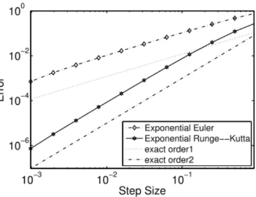
Figure 1: The error of the exponential Euler method of order one and the exponential Runge–Kutta method of order two when applied to (68) with200grid points. For comparison, we added lines with slope one and two.
Table 1: The Table clearly demonstrates the numerically observed temporal orders of convergence in theL2 norm withM grid points andh= 1/128. Herer= 0.05, E= 100, σ= 0.2, λ= 2, T = 1.
M Exponential Euler method Exponential Runge–Kutta method
50 1.0660 2.0159
100 1.0650 2.0149
200 1.0644 2.0141
where
A4=
1 2σ
2∂2u
∂x2, A3 = (r−
1 2σ
2−λκ)∂u
∂x, A2=−(r+λ)u.
Figure 1 clearly elucidates the convergence of computed first order exponential Euler method and second order exponential Runge-Kutta method for constant time steps with 200 grid points. The computed solution for exponential Euler converges at a first-order and for exponential RungeKutta as second-order rate, as one can see undoubtedly from Figure 1. The errors are measured in the L2 norm. For comparison, we added the lines with slope one and slope two.
The numerical values are shown in Table 1 for the temporal orders of convergence in the L2 norm with M grid points and h = 1/128, for the PIDE (68) in case of the exponential Euler method of order one and the exponential RungeKutta method of order two.
5. Concluding remarks
References
[1] A. Almendral and C.W. Oosterlee. Numerical valuation of options with jumps in the underlying. Appl. Numer. Math., 53:1–18, 2005.
[2] R. Cont and E. Voltchkova. Finite difference methods for option pricing in jump-diffusion and exponential l´evy models. Rapport interne 513(September), CMAP, 2003.
[3] A. Gopaul D.Y. Tangman and M. Bhuruth. Exponential time integration and cheby-chev discretization schemes for fast pricing of options. Appl. Numer. Math., 58:1309– 1319, 2008.
[4] M.A. Gondal. Exponential Rosenbrock integrators for option pricing. J. Comput. Appl. Math., 234:1153–1160, 2010.
[5] M.A. Gondal. Convergence of an exponential Euler method for option pricing. World Applied Sciences Journal, 14:1816–1822, 2011.
[6] M.A. Gondal. Option valuation in jump diffusion models using the exponential Runge-Kutta methods. World Applied Sciences Journal, 13:2396–2404, 2011.
[7] D. Henry. Geometric theorey of semilinear parabolic equations, Lecture notes in Math.840. Springer, Berlin, Heidelberg, 1981.
[8] M. Hochbruck and A. Ostermann. Explicit exponential Runge–Kutta methods for semilinear parabolic problems. SIAM J. Numer. Anal., 43:1069–1090, 2005.
[9] M. Hochbruck and A. Ostermann. Exponential Runge–Kutta methods for parabolic problems. Appl. Numer. Math., 53:323–339, 2005.
[10] M. Hochbruck and A. Ostermann. Exponential Integrators. Acta Numerica, 19:209– 286, 2010.
[11] J.Loffeld and M.Tokman. Comparative performance of exponential, implicit, and explicit integrators for stiff systems of ODEs. Journal of Computational and Applied Mathematics, 245:45–67, 2013.
[12] Ch. Lubich and A. Ostermann. Runge–Kutta time discretization of reaction-diffusion and Navier–Stokes equations: nonsmooth-data error estimates and applications to long-time behaviour. Appl. Numer. Math., 22:279–292, 1996.
[13] C.La Chioma M. Briani and R. Natalini. Convergence of numerical schemes for viscos-ity solutions to integro-differential degenerate parabolic problems arising in financial theory. Numerische Mathematik, 98:607–646, 2004.
[15] A. Ostermann and M. Thalhammer. Non-smooth data error estimates for linearly implicit Runge–Kutta methods . IMA J. Numer. Anal, 20:167–184, 2000.
[16] A. Pazy. Semigroups of linear operators and applications to partial differential equa-tions. Springer, New York, 1983.
[17] M.N. Le Roux. Semidiscretization in time for parabolic problems. Math. Comput., 33:919–931, 1979.
[18] J.A. Pudykiewicz V.T. Luan and D.R. Reynolds. Further development of efficient and accurate time integration schemes for meteorological models. Journal of Com-putational Physics, 376:817–837, 2019.